Abstract
Climate change significantly influences changes in ecological phenomena and processes, such as species distribution and phenology, thus accelerating the rate of species extinction or prosperity. Climate change is considered to be one of the most important threats to global biodiversity in the 21st century and will pose significant challenges to biodiversity conservation in the future. The use of niche modelling to predict changes in the suitable distribution of species under climate change scenarios is becoming a hot topic of biological conservation. In this study, we use data from China’s National Forest Continuous Inventory as well as specimen collection data of Cunninghamia lanceolata (Lamb.) Hook to run optimized Maxent models to predict potential suitable distribution of the species in the present day, 2050s, and 2070s under different climate change scenarios in China. In the modeling process, the most important uncorrelated variables were chosen, and the sample-size-adjusted Akaike information criterion (AICc) was used to select the optimal combination of feature type and regularization multiplier. Variable selection reduced the number of variables used and the complexity of the model, and the use of the AICc reduced overfitting. Variables relating to precipitation were more important than temperature variables in predicting C. lanceolata distribution in the optimal model. The predicted suitable distribution areas of C. lanceolata were different for the different periods under different climate change scenarios, with the centroids showing a degree of northward movement. The suitable distribution area is predicted to become more fragmented in the future. Our results reveal the climate conditions required for the suitable distribution of C. lanceolata in China and the likely changes to its distribution pattern in the future, providing a scientific basis for the sustainable management, protection, and restoration of the suitable habitat of this economically important tree species in the context of climate change.
1. Introduction
Climate is the main factor determining the distribution pattern of plants, and changes in this distribution pattern are a direct reflection of climate change [1,2,3,4,5]. The Fifth Assessment Report (AR5) of the Intergovernmental Panel on Climate Change (IPCC) indicates that the annual mean temperature of the Earth’s surface has increased by 0.85 °C over the past 130 years (1880–2012). While the mean temperature of the past 60 years (1951–2012) has increased by 0.72 °C. The mean global surface temperature is predicted to increase by an additional 0.3–4.8 °C by the end of the 21st century, according to simulations of greenhouse gas emission scenarios [6]. Several observational studies have shown that climate change has caused or is causing significant changes to ecological processes, including distribution ranges, morphological characteristics, and phenology that are accelerating species extinction or prosperity [7,8,9]. Because of this, quantitative analysis of climate factors and predictions of climate change impacts on potential suitable species distributions have become key to biogeography and global change research [8,10,11].
Niche modelling (also known as species distribution modelling or habitat suitability modelling) uses statistical or biophysical methods to infer the environmental requirements for the survival of a species based on the environmental variables taken from the known distribution areas, and then predicts their potential or future distribution [12,13,14]. Niche modelling has been widely used in ecology, biogeography, and conservation biology studies, such as the adaptive analysis of invasive alien species [15,16], conservation of endangered species [17,18], selection of natural reserves [19,20], and impacts of climate change on species distribution [21,22,23]. At present, there are many niche models used for species distribution prediction, including the bioclimate analysis and prediction system (BIOCLIM) [24], the genetic algorithm for rule set production (GARP) [25], the ecological niche factor analysis (ENFA) [13], and the Maximum Entropy Model (Maxent) [26,27]. These niche models, established on the basis of the statistical relationship between species distribution and environment variables (rather than the causality), only consider the environmental factors that control species distribution and do not consider the interactions between species, species evolution, extreme interference events, or species diffusion processes [12,28]. The current correlation between species and the environment (climate) does not necessarily guarantee that it can be used to predict future species distribution; however, niche modelling is still the most commonly used method for assessing the impacts of climate change on species distribution at the regional scale. Niche modelling is required to predict changes in species distribution, due to the difficulty of effectively carrying out field experiments at the geographical distribution scale of an entire species [28,29]. Niche models can be easily constructed and can provide rapid predictions for the changes to species distribution and the risk of habitat loss.
The Maxent model, which is based on the theory of maximum entropy, is an effective model of species distribution. The model simulates the potential geographical distribution of a species using information on its current (present day) distribution as well as various environmental data [27,30]. The Maxent model is relatively simple and quick to run, has a small sample demand, provides stable operation results, and allows prediction results to be tested [27,31,32]; thus, it is favored by many researchers [14,33,34]. However, the model is often employed using the default parameters or those published previously without consideration of the details of the algorithm or input parameters, and all the environment variables that can be collected are included in the model indiscriminately. This not only increases the complexity and operation time of the model, but also greatly limits its scope of application and accuracy. Previous studies have shown how different environmental variables and parameters used in niche models affect the results [35,36,37]. Complex models show low performance in identifying the most important environmental variables and in transferring habitat suitability to new environmental conditions [38,39,40]. When using the default parameters of the Maxent model to predict the potential suitable distribution of species, overfitting can occur, leading to a decline in species-transfer ability [41,42]. Therefore, the selection of appropriate environmental variables and model parameters is an important step that must be considered in the application of the Maxent model.
Cunninghamia lanceolata (Lamb.) Hook is a fast-growing and high-yielding tree that is native to the subtropical region of South China, where it is the main species used in afforestation and for timber production. It is a long-lived evergreen tree and plays an important role in regional ecological construction. Therefore, it is important to study the impact of climate change on the suitable habitat of C. lanceolata. In this study, the Maxent model is used to simulate the suitable distribution of C. lanceolata and how this might change under different climate change scenarios after parameter optimization and climate variable selection. The specific objectives of this study are as follows: (1) to explore the influence of environmental variable selection and parameter settings on the performance of the Maxent model; (2) to understand the importance of environmental variables in predicting the potential suitable distribution of C. lanceolata; and (3) to compare the differences in the predicted distribution of C. lanceolata under different climate change scenarios in different time periods. Our optimized model, based on the variables with the highest explanatory power, reveal the climate conditions required by C. lanceolate that account for its present-day distribution. The model also suggests marked changes to this distribution pattern under predicted climate change scenarios and increased fragmentation of suitable habitat by the 2070s.
2. Materials and Methods
2.1. Data
2.1.1. Species Occurrence Data
Species occurrence data from the basis of potential suitable distribution predictions under climate change scenarios in niche modelling and the accuracy and reliability of the occurrence data are directly related to the plausibility of the predicted results [43,44]. Two sources of C. lanceolata occurrence data were used for this study: (1) the National Forest Continuous Inventory (NFCI) of China; and (2) records of specimen collection of the China National Specimen Information Infrastructure (NSII) and the Chinese Virtual Herbarium (CVH). The NFCI is the first level of the forest inventory system of China designed to provide reliable data on the current status of, and changes in, forests in the form of an integrated spatial database [45]. The NFCI survey is carried out every five years at the provincial scale. The permanent sample plots are systematically located at the graticule intersection of the national topographic map (scale 1:100,000 or 1:50,000) [46]. The NFCI data are the only high-quality forest inventory data available at the national scale at present [47]. The NFCI plots, in which the dominant tree species was C. lanceolata, were selected. Records of collected C. lanceolata specimen that had accurate associated coordinates were obtained from the China National Specimen Information Infrastructure (NSII) [48] and the Chinese Virtual Herbarium (CVH) [49]. We selected only one point closest to the center in the 30” grid plots (approximately 1 km2), which was matched with climate data layers, to reduce spatial autocorrelation [50]. In total, 1307 NFCI points and 570 specimen record points were obtained for niche modelling (Figure 1).
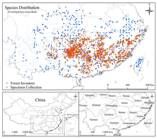
Figure 1.
Distribution of the occurrence points of Cunninghamia lanceolata in China. Orange points represent data from The National Forest Continuous Inventory (NFCI) of China and blue points represent collected specimen data from the China National Specimen Information Infrastructure (NSII) and Chinese Virtual Herbarium (CVH).
2.1.2. Climate Data
Environmental variables were selected according to their relevance to plant survival and growth, thus precipitation and temperature are the primary environmental factors affecting plant distribution, since the formation of the plant distribution pattern is closely associated with the precipitation and temperature [51]. The climate data used in the prediction of suitable species distributions under climate change scenarios included the baseline climate condition data (time period: present day [average for 1970–2000]) and the climate scenario data (time periods: 2050s [average for 2041–2060] and 2070s [average for 2061–2080]). The baseline climate condition data were obtained using a thin plate spline function to establish the relationship between the observation values (24,254 mean temperature observatories, 14,835 minimum and maximum temperature observatories, and 47,554 precipitation observatories) and the corresponding latitude, longitude, and elevation of the observatories; the data were then interpolated to the area without the original observation values [52]. The climate scenarios for the 2050s and 2070s were derived from the downscaled global climate model (GCM) of the IPCC AR5. The Beijing Climate Center Climate System Model version 1.1 (BCC-CSM1-1), developed by the Beijing Climate Center of China Meteorological Administration, provided the data on China for the IPCC AR5 [53,54]. The BCC-CSM1-1 included data on four climate change scenarios under the different Representative Concentration Pathways (RCPs), which had a high temperature and precipitation prediction accuracy, and included detailed consideration of the impact of greenhouse gas emissions through various policies and strategies for coping with global climate change [6]. The four RCPs (RCP2.6, RCP4.5, RCP6.0, and RCP8.5) are defined by the possible range of radiative forcing values (2.6, 4.5, 6.0, and 8.5 W/m2, respectively) in the year 2100 [6]. Previous work has indicated that the RCPs of BCC-CSM1-1 have a high accuracy for China [55]; thus, the RCP data from the BCC-CSM1-1 was used to predict future suitable distributions of C. lanceolata in this study.
The climate variable data used in this study can be downloaded from the WorldClim-Global Climate Data website [56]. The data includes 19 climate variables, which were derived from the monthly temperature and precipitation values to generate more biologically meaningful data that reflect a range of temperature and precipitation summaries (e.g., trends, seasonality, and extremes) [57]. The spatial resolution of the data was 30” (approximately 1 km2). The description and statistics of these climate variables are presented in Table 1 and Table A1, respectively.

Table 1.
Climate variables used for niche modelling.
2.2. Model
The Maxent model is a niche modelling based on the maximum entropy theory [27]. Maximum entropy theory, proposed by Jaynes, in 1957, holds that anything with the maximum entropy is closest to its real state under known conditions [58]. The Maxent model is used to estimate the target probability distribution by finding the probability distribution of the maximum entropy (i.e., that is most spread out, or closest to uniform) that is subject to a set of constraints that represent our incomplete information regarding the target distribution [27]. In a study of species’ distribution, the constraints are climate, soil, terrain, or other environmental variables influencing the species’ occurrence points. Maxent software was developed by Phillips et al., in 2004 [26].
2.3. Optimization of Model Parameters
The Maxent model was used to predict the potential suitable distribution of C. lanceolata in three time periods (present day, 2050s, and 2070s). The predictive performance of the model is influenced by the choice of two parameters that need to be optimized: (i) the regularization multiplier (RM), and (ii) the feature combination (FC). RM can affect how focused the output distribution is. A smaller RM value will result in a more localized output distribution that fits the given occurrence records better, but is more prone to overfitting. Overfitted models are poorly transferable to novel environments and, thus, not appropriate to project distribution changes under environmental change. A larger RM value will produce a prediction that can be applied more widely [27,30]. We used RM constants of 0.5 to 5 with steps of 0.5.
The features, which were produced from the climate variable layers, constrain the computed probability distribution. The available feature types include linear (L), quadratic (Q), product (P), threshold (T), and hinge (H). The functions of these feature types are as follows [27,30]:
- (1)
- Linear features constrain the output distribution for each species to have the same expectation of each of the continuous climate variables as the sample locations for that species. A linear feature is simply one of the continuous climate variables.
- (2)
- Quadratic features (when used together with linear features) constrain the output distribution to have the same expectation and variance of the climate variables as the samples. A quadratic feature is the square of one of the continuous climate variables.
- (3)
- A product feature is the product of two continuous climate variables; when used with linear and quadratic features, product features constrain the output distributions to have the same covariance for each pair of climate variables as the samples.
- (4)
- A threshold feature is derived from a continuous climate variable. For a threshold value v, the threshold feature is binary (taking values 0 and 1) and is 1 when the variable has value greater than v. The effect of a threshold feature is to make the total probability of grid cells with a value greater than the threshold be equal to the fraction of sample locations with the value above the threshold v.
- (5)
- A hinge feature is also derived from a continuous environmental variable. It is like a linear feature, but it is a constant below a threshold v.
The default RM value is 1. The selection of FC is related to the number of species occurrence points. Generally, linear features are always used in the model, quadratic features are used when the number of occurrence points are more than 10, hinge features are used when the number of occurrence points are more than 15, and threshold and product features are used when the number of occurrence points total more than 80 [59]. Two feature types and five FCs (i.e., L, H, LQ, LQH, LQP, LQHP, and LQHPT) were used in this study.
The grid search approach (i.e., an exhaustive search method for setting parameter values) was used to find the best combination of RM and feature type—i.e., the performance of the 70 models (run using different combinations of RM and feature type) was compared.
2.4. Variable Selection
Along with the selection of the combination of RM and feature type, the complexity of the Maxent model should also be considered. Generally, the accuracy of simple niche models is low but the transferability to novel climate conditions is high, while the opposite is true for complex models [36,38,60]. The number of climate variables affects the complexity of the Maxent model. On the one hand, too many climate variables will affect the calculation time and efficiency when predicting the suitable distribution of species on a large regional scale; on the other hand, the climate variables with obvious collinearity will affect the interpretation of the results. Therefore, it is particularly important to reduce the number of climate predictor variables and select the appropriate ones to improve the transferability of the Maxent model to different climate change scenarios. Data dimensionality reduction methods such as correlation analysis and principal component analysis are widely used in the selection of climate variables before the prediction of suitable habitats for species [61,62,63]. However, these methods of variable selection before modeling cannot effectively identify which variables are most important for the predictions using the Maxent model.
Maxent provides two metrics to determine the importance of input climate variables in the final model: percent contribution and permutation importance [27]. Each step of the Maxent algorithm increases the gain of the model by modifying the coefficient for a single variable, and the program can assign the increase to the climate variables that the variable depends on; the percent contribution is obtained at the end of the training process by converting the increase to a percentage [64]. The permutation importance of each variable is determined by randomly permuting the values of that variable among the training points and measuring the resulting decrease in training of the curve of the receiver-operating characteristic plot, with a large decrease indicating that the model depends heavily on that variable [64].
In this study, the climate variables were selected on the basis of their percent contribution. However, the interpretation of variable contributions is unsuitable when the predictor variables are correlated [27]. Therefore, the correlation between the variables was also considered to exclude those with high correlations with the important contributing variables. The acquisition of the suitable variable subset was a continuous search process consisting of four steps:
- (1)
- Subset generation: generation of a candidate variable subset according to a certain search strategy. We used a generalized sequential backward selection approach where variables were continuously excluded from the start point of the search (the original full variable set). First, an initial Maxent model was compiled with all climate variables included. Then, all variables that had a percent contribution score below the set value of contribution threshold were removed. Variables that correlated with the variable showing the highest percent contribution above the set value of correlation coefficient threshold were then excluded. The remaining variable set was used to compile a new Maxent model.
- (2)
- Stopping criterion: used to determine when the variable search algorithm should stop. The process of subset generation was repeated until the variable subset met the stopping criterion. The search process stopped only when the variable subset met two criteria: (i) the percent contribution score of variables must be above the contribution threshold (equal to 1); and (ii) the correlation of variables must be below the correlation coefficient threshold (equal to 0.9).
- (3)
- Subset validation: used to verify the validity of the selected variable subset. A 10-fold cross-validation approach was performed to evaluate the performance of the variable subset in each round; therefore, the subset validation was not an independent step in the process.
- (4)
- Subset evaluation: evaluation of the prediction performance of the final variable subset through an evaluation function. We used two main evaluation criteria: (i) the sample-size-adjusted Akaike information criterion (AICc) [65]; and (ii) the area under the curve (AUC) estimated from test data [66].
The R package dismo [67] was used to run the Maxent software (Version 3.4.1, Cambridge, MA, USA) which performed the Maxent modeling and variable selection. The contribution of the variables was obtained using the jackknife approach [68]. The correlation between the climate variables was calculated using the Pearson correlation coefficient in the software SPSS (Version 25, Armonk, NY, USA) (Table A2). Each model runs using a combination of RM and feature type needed to search the variable subset. The variable selection workflow is shown in Figure 2.
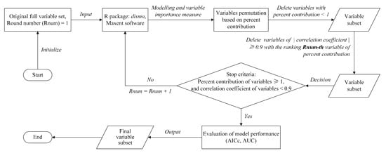
Figure 2.
Workflow of the variable selection based on variable importance and correlation for the Maxent models.
2.5. Evaluation Criteria
Evaluation of model performance is an important topic in niche modelling [69]. In the Maxent model, the AUC of the receiver-operating characteristic plot is used as a default evaluation criterion to assess the accuracy of the model. The AUC, which is a threshold-independent evaluation criterion that is not sensitive to species prevalence [70], is widely used in niche modelling [23,27,66,71]. Generally, the AUC value ranges from 0.5 to 1, and the higher the value, the better the prediction of the model. Five grades of model prediction accuracy can be classified according to the AUC value [72]: 0.5–0.6, fail; 0.6–0.7, poor; 0.7–0.8, fair; 0.8–0.9, good; and 0.9–1, excellent.
However, it has been suggested that high AUC values are associated with the degree to which a model can successfully distinguish occurrence from background localities, but this rank-based non-parameter metric cannot be used to evaluate the model goodness-of-fit [73,74]. That is, the maximization of test AUC values favors models that can discriminate between occurrence and background sites well but may overfit the realized niche of a species [38,66]. Therefore, using multiple evaluation criteria to reduce the deficiency of single evaluation criterion has become a popular method for evaluation of the niche modelling [75,76].
The AIC, based on the entropy theory, is a criterion to measure the goodness-of-fit of a statistical model and can weigh the complexity of the estimated model [65]. The AICc was developed by Warren et al. [38,40] as an AIC corrected for small sample size; however, it has been widely used regardless of sample size based on the recommendation of Burnham et al. [77]. The AICc is calculated based on the unpartitioned (full) dataset [78]:
where k is the number of parameters in the model (i.e., number of non-zero parameters in the Maxent lambda file) which record the coefficients of the Maxent model for a species; n is the number of occurrence localities; v is a vector of Maxent raw values at occurrence localities; and t is the sum of Maxent raw values across the entire study area. The AICc was calculated using the “calc.aicc” function in the R package ENMeval [79].
Generally, minimization of AICc values favors models that recognize the fundamental niche of a species and that are more transferable to future climate scenarios [38]. Therefore, the minimal AICc value has been used to select the optimal model in numerous studies [80,81,82].
In addition, a relative measure (i.e., the difference between training and testing AUC values [AUC.Diff]) was also used to quantify the degree of overfitting. The AUC.Diff is expected to be high for models overfit to the training data [38].
2.6. Division of Suitable Distribution Area
The suitable distribution area was divided into three grades using the Jenks’ natural breaks approach according to the value of suitability in previous studies [83,84]: 0–0.25, non-suitable area; 0.25–0.5, low-suitability area; and 0.5–1, high-suitability area. However, the natural breaks approach did not produce clear divisions of suitable distribution areas and the area defined as high-suitability was too large, which hinders detailed analysis for a species. Therefore, five grades of suitable distribution area were classified using the equal interval approach: 0–0.2, non-suitable area; 0.2–0.4, low-suitability area; 0.4–0.6, general-suitability area; 0.6–0.8, medium-suitability area; and 0.8–1, high-suitability area.
The change in suitable distribution area is a common species distribution analysis criterion. The size of the suitable area plays an important role in maintaining the spatial continuity of a species, but the structure and function of a suitable area are also important aspects. Therefore, we used four landscape metrics—aggregation index (AI), fractal dimension index (FRAC), Shannon’s diversity index (SHDI), and contagion (CONTAG)—to evaluate spatial pattern change in suitable areas from a landscape aspect (Table A3). The AI and FRAC are class metric measures that aggregate properties of the patches belonging to a single class in the landscape, while SHDI and CONTAG are landscape metrics that measure the aggregate properties of the entire patch mosaic. These landscape metrics are calculated by the software FRAGSTATS: Spatial Pattern Analysis Program for Categorical Maps (Version 4.2, Amherst, MA, USA).
In addition, the direction and range of the species migration under the climate change scenarios were analyzed by comparing changes to the location of the suitable-area centroid.
3. Results
3.1. Variable Selection and Accuracy Evaluation
Figure 3 shows how the performance of the Maxent models altered when different combinations of RM and feature type were included after variable selection. Variable selection could significantly reduce the number of variables included, but the models with a low RM or a complex combination of feature type required more variables. Thirteen variables were selected which differed in importance. Bio2, Bio6, Bio8, Bio12, Bio14, and Bio15 were frequently selected, highlighting the importance of these variables in Maxent models of C. lanceolata.
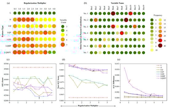
Figure 3.
The results of variable selection and three evaluation metrics of the Maxent models run using different combinations of regularization multiplier and feature type. (a) Selected variable count of the models. (b) Frequency of selected variables with ordering based on percent contribution. (c) Sample-size-adjusted Akaike information criterion (AICc) score. (d) Test area under the curve (AUC) score. (e) Difference between training AUC and test AUC (AUCtrain − AUCtest) values. Default settings and those that yielded the lowest AICc are indicated with red and black arrows, respectively. Feature classes: L, linear; H, hinge; Q, quadratic; P, product; and T, threshold.
The evaluation metric result showed that the test AUC values of all models were larger than 0.86, suggesting that the models worked well and had high prediction accuracy, but the values of change were not too large. By contrast, the minimum AICc value of the model (RM = 3.5, FC = LQH) was significantly lower than the default model value (RM = 1, FC = LQHPT). The AUC.Diff value of the default model was larger than the minimum AICc value, indicating that the default model was overfitted to the training data. Additionally, the number of variables of the model with the minimum AICc value (variable count = 5) was also lower than the default model (variable count = 7). Therefore, to reduce the overfitting and complexity, the model with the minimum AICc was selected as the optimal model to predict the suitable distribution area for the present day, 2050s, and 2070s under different climate scenarios in China (Table 2).
Table 2.
Evaluation metrics of the default and optimal Maxent models.
3.2. Variable Importance
Five variables were included in the optimal model: Bio14 (precipitation of driest month), Bio12 (annual precipitation), Bio6 (min temperature of coldest month), Bio8 (mean temperature of wettest quarter), and Bio5 (max temperature of warmest month) (Table 3). The cumulative contribution (i.e., importance) of Bio14 and Bio12 was more than 90%, rising to over 95% with the inclusion of Bio6, indicating that these variables best explain the data. Therefore, precipitation variables appear more important to the Maxent predictions for C. lanceolata than temperature variables. The selected variables determining the suitable distribution of C. lanceolata represent near-extreme climate variables. To understand how these variables affected the predicted distribution of C. lanceolata, the response curves were calculated to estimate the relationship between the probability of presence and climate factors.
Table 3.
Contribution (i.e., important) parameters of the five climate variables included in the optimal model.
The red lines in Figure 4 show how the variables affect the predicted probability of suitable conditions when all other variables are set to their average value; that is, the curves showed the marginal effect of changing only one variable. High correlations between the variables after variable selection was not observed (Table A2), and thus, the marginal response curves can be interpreted. The probability of presence value increased with increasing Bio14, Bio12, and Bio6 values, before stabilizing at a high probability, or decreased after reaching the maximum probability; this indicates the importance of these variables for predicting distribution patterns of C. lanceolata. By contrast, the probability value was high for most Bio8 and Bio5 values although it decreased rapidly at high variable values; however, the roles these variables were not obvious and the significance of other variables to the optimal model suggests that they are not of high importance in predicting distribution patterns.
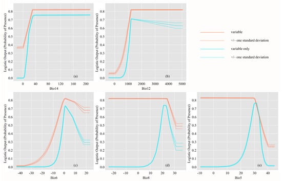
Figure 4.
Response curves characterizing how each variable affected the Maxent predictions. Red lines show how the logistic prediction changed as each climate variable was varied while keeping all other variables at their average sample value. Blue lines illustrate Maxent models created using only the corresponding variable. Solid lines represent the mean response of 10 replicate Maxent runs while dashed lines represent the mean ± one standard deviation.
The blue lines in Figure 4 show how each of the five optimal-model variables independently affect the predicted probability of suitable conditions, namely, a Maxent model created using only the corresponding variable. The probability of presence of C. lanceolata is close to 0 when the precipitation of the driest month (Bio14, the most significant variable), is less than 5 mm, then increases rapidly and reaches the maximum when Bio14 is over 30 mm. Similarly, the probability of presence is close to 0 when annual precipitation (Bio12) is less than 500 mm, then increases rapidly and reaches the maximum when Bio12 is over 1200 mm. Therefore, there appears to be no upper limit but a strict lower limit of precipitation variable values for the suitable distribution area of C. lanceolata. According to the suitability grade, the suitable distribution area (probability ≥0.6) for C. lanceolata requires more than 20 mm of precipitation during the driest month and an annual precipitation of over 1100 mm. In contrast to the precipitation factors, the suitable distribution area of C. lanceolata has strict upper and lower temperature limits. The probability of presence was close to 0 when Bio6 (min temperature of coldest month), Bio8 (mean temperature of wettest quarter), and Bio5 (max temperature of warmest month) were less than −15 °C, 5 °C, and 10 °C, respectively, before increasing rapidly and reaching the maximum level when these values rose to 2 °C, 23 °C, and 33 °C, respectively, again showing a sharp drop-off above these values. According to the suitability grade, the suitable distribution area (probability ≥0.6) for C. lanceolata requires the minimum temperature in the coldest month, mean temperature of the wettest quarter, and maximum temperature of the warmest month to be 0–8 °C, 19–25 °C, and 28–34 °C, respectively.
3.3. Analysis of Potential Suitable Distribution
The present-day predicted suitable distribution area of C. lanceolata was situated in Guizhou, Hunan, Guangdong, and Fujian Province, coincident with the actual distribution (Figure 5). The percent of area of general-, medium-, and high-suitability distribution was 6.86%, 5.25%, and 0.76%, respectively (Table 4). The suitable distribution areas markedly changed for different time periods under different climate change scenarios. Compared to the present-day predictions, the total area of suitable distribution (general-, medium-, and high-suitability) gradually decreased in the 2050s and 2070s (Table 4). The ranking of the total area under different climate change scenarios was RCP2.6 > PCP4.5 > PCP6.0 > PCP8.5, indicating that as the greenhouse gas emissions increase, the distribution of C. lanceolata is likely to decrease. It is of note that the area of high-suitability distribution for RCP4.5 greatly increased in the 2050s.
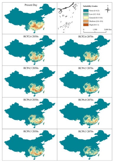
Figure 5.
Prediction of potential suitable distribution area for Cunninghamia lanceolata during the present day, 2050s, and 2070s under different climate scenarios in China. RCPs: Representative Concentration Pathway data defined by the possible range of radiative forcing values (2.6, 4.5, 6.0, and 8.5 W/m2, respectively) in the year 2100 taken from the Beijing Climate Center Climate System Model version 1.1 (BCC-CSM1-1) included in the IPCC Fifth Assessment Report (AR5).
Table 4.
Percentage of the predicted suitable area for the presence of Cunninghamia lanceolata for the present day, 2050s, and 2070s under different climate scenarios in China. RCPs: Representative Concentration Pathway data defined by the possible range of radiative forcing values (2.6, 4.5, 6.0, and 8.5 W/m2, respectively) in the year 2100 taken from the Beijing Climate Center Climate System Model version 1.1 (BCC-CSM1-1) included in the IPCC Fifth Assessment Report (AR5).
Because the edges of the suitable distribution area were not regular, it is more suitable and representative to express their change using the centroid movement. The centroids of the suitable distribution area were located in Hunan and Jiangxi Provinces and showed a degree of northward movement compared to the present-day position under different climate change scenarios (Figure 6). However, the distance of centroid movement differed between suitability grades in different time periods. The movement distance of the general-suitability grade was smaller than the medium grade, which was in turn smaller than the high-suitability grade and the predicted movement distance was greater in the 2070s than in the 2050s. Therefore, the distance of centroid movement was positively correlated with the range of change between the different climate change scenarios and the present day (Table 4), indicating that the larger the moving distance of the centroids, the greater the change of the suitable distribution area. In addition, the centroids of the high-suitability distribution area for RCP2.6, RCP4.5, and RCP8.5 in the 2070s show a clear eastward progression compared to the 2050s.
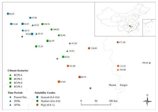
Figure 6.
Centroid distributions of general-, medium-, and high-suitability areas for Cunninghamia lanceolata for the present day, 2050s, and 2070s under different climate change scenarios. Point numbers represent the distance (km) between the predicted and present-day centroids. Cimate scenarios are distinguished by a given symbol; for time periods, present day is displayed by a star, and 2050s and 2070s are distinguished by the center of symbols; suitability grades are distinguished by the color.
The general-, medium-, and high-suitability distribution areas were predicted as more fragmentated in the 2050s and 2070s compared to the present day (Figure 5). The landscape metric results also indicated that the suitable distribution areas will become increasingly fragmented (Table 5). For the class metrics, the AI values of the general-, medium-, and high-suitability distribution areas gradually decreased from RCP2.6 to RCP8.5, indicating that the predicted patches became more discrete; conversely, the FRAC values of these classes gradually increased, suggesting that the predicted edges of these patches became more complex. Because the areas of non-suitable distribution increased, the CONTAG values also gradually increased while the SHDI values gradually decreased. Although these metrics express the structural characteristics of different suitability grades from different aspects, they all predict that the suitable area of C. lanceolata will gradually decrease or even be lost altogether as a consequence of climate change.
Table 5.
Landscape metrics of the suitable distribution area for Cunninghamia lanceolata for the present day, 2050s and 2070s under different climate change scenarios.
4. Discussion
Niche modelling is a powerful tool for the prediction of potential species distribution that can help inform applied ecology. However, there are several limitations to niche modelling, such as low transfer ability and discrepancies between the simulation results and the actual species distribution, that can result in an inappropriate conclusion being drawn from the models. Improving the transfer ability of niche models not only helps to accurately simulate the potential species distribution, but can also generate important reference data for theoretical issues such as niche conservation.
Maxent has been widely used in the prediction of potential distribution of species in recent years [34,85]. The model assumes that species will be present in all areas with suitable climate conditions and will not present in any area with unsuitable conditions; it is believed that the larger the entropy of a species under known conditions, the closer it is to the reality [27]. The default parameters of Maxent were originally set through the testing of data from 266 species in six different geographical regions by early model developers [30]. They used the massive distribution data of the test species and a variety of experimental schemes to define optimal model parameters as the default to promote and simplify the application of the model; however, the purpose of application of these models was to predict the present-day distribution of a species, and the model did not have to be transferable after construction [30,86]. Adjustments to the simulation scheme are necessary to meet different simulation requirements depending on the research question, although the species distribution simulated by the Maxent model is between the potential distribution and the real distribution [86]. To simulate the potential distribution of a species, the default parameters of the Maxent model may not be applicable. For example, the parameters of our optimal model differ from the default parameters (Figure 3, Table 2). If only the default parameters are used, the transfer of the model will be reduced because of overfitting, although it can fit the current distribution of the species for the study area well.
The complexity of a Maxent model has a significant influence on its transfer ability. Both simple and complex models have advantages and disadvantages. Simple models may show a poor fit to the species distribution data of the study area, and while complex models can produce a better fit, the response relationship between species and environmental variables can deviate from the reality. The adverse effect of Maxent model complexity on prediction results when simulating potential distributions is more serious because of the need to transfer the model to other geographical areas after model construction [38,40]. The prediction ability of complex models will be reduced, and the simulation results may not be reliable or can deviate from the actual situation, because of overfitting when they are transferred to other geographical areas.
In this study, steps were taken to optimize the two main factors known to influence the prediction results of the Maxent model. First, as much species distribution data as possible were collected to reduce error caused by incomplete data collection; a total of 1877 sample points were collected. Generally, the species distribution points should not only adequately cover the geographical distribution and ecological space of a species, but also reduce the inaccuracy of sampling points. It has been shown that the sample size of species distribution data significantly affects the accuracy of model simulation results [87,88,89,90]. In this study, the modeling data covered the southern provinces of China and only one point was reserved in the same pixel. Second, we optimized the parameters of the model. We constrained the complexity of the model by reducing the number of variables through variable selection and using AICc values to select the optimal combination of feature types and RM. Along with decreasing the complexity of the model, reducing the number of variables can reduce the operation time and improve the interpretability. The Maxent model uses the default criterion (i.e., the AUC) to evaluate the prediction ability of the model, but the AUC may overestimate this ability and directly affect the species distribution results when test data and training data are affected by sampling error [40,91]. Nevertheless, using the AICc to select the feature type and the built-in RM can constrain the complexity of model [38].
Five factors (i.e., climate change, habitat change, overexploitation, pollution, and invasive alien species) are viewed as the principal threat to global biodiversity in the 21st century [92]. As an important aspect of global change, climate change mainly manifests as temperature rises, changes to precipitation patterns, and increasing extreme climate events; in addition, changing climate factors will also affect the growth and reproduction, phenology, and geographical distribution of species at the regional scale [1,2,93]. Current biodiversity conservation measures, such as the establishment of nature reserves, are usually based on the current distribution of species, but are facing increasing challenging as the effects of climate change increase [20,94]. It is of key importance to understand changes in suitable areas of distribution under the future climate change scenarios, and implement targeted conservation measures as early as possible to improve the effectiveness of biodiversity conservation [29,95]. With the exponential growth of global greenhouse gas emissions, the trend of climate warming in China will be further intensified in the future. The results of this study show that climate change will have a significant impact on the suitable distribution area of C. lanceolata, and the suitable habitat area will likely gradually decrease. In addition, we found that the prediction results using RCP4.5 data were different from other climate scenarios. Previous studies have shown that the climate scenario of RCP4.5 is the closest to the actual predicted climate situation in China [55]; thus, the suitable distribution area of C. lanceolata has not been significantly reduced over a short time period under this climate scenario. However, the suitable distribution area of C. lanceolata will still likely see a large reduction with the likely effects of climate change caused by continuing increases in greenhouse gas emissions.
Climate change, especially global warming, not only causes temperature changes in different regions, but also changes the distribution pattern of precipitation. When the change of these climatic factors is close to or beyond the adaptive threshold of current plant growth, it will lead to the migration of their distribution [7]. Water availability has a significant impact on plant height, leaf area, branch number, photosynthesis and growth [96], thus, precipitation can constrain species distribution and influence distribution in various ways [97]. The increase of precipitation during the driest month results in a longer growth season and helps species migrate to more suitable habitats within their distribution [98]. In addition, extreme high and low temperatures also have a significant influence on plant growth. The decrease of the minimum temperature of the coldest month results in premature freezing injuries to plants, and long-term low temperatures will lead to the death of plants at the distribution limit [97]; while the increase of the maximum temperature of the warmest month will destroy the water balance of plants, promote the coagulation of proteins and the internal mechanism of harmful metabolites, thus hindering plants’ growth [99]. Climate extremes have been shown to have important impacts on species’ distribution and diversity, and adding extreme climate variables in niche modelling can improve the predicted accuracy and limit of species distributions under future climate change scenarios [100,101,102,103,104].
Because of changes in environmental factors, particularly those of the climate, the suitable habitat of tree species has changed in China, which makes it difficult to correctly formulate a long-term forest management plan. Sustainable forest management planning at the regional scale includes predicting the spatial distribution of different types of forests and forest management division; it is therefore a spatial decision-making process. The impact of forest management on ecosystems and the evaluation of forest management effectiveness are long-term processes; therefore, a long-time scale must be adopted to measure the sustainability of forest management. When developing forest management plans, optimized model simulations and decision analysis of the management process should be carried out over at least one forest management cycle. During the process of long-term (>30-year) forest management planning, climate change will lead to changes in the environment, and thus suitable habitats, for tree species. Therefore, it is necessary to consider the impact of climate change in the process of long-term forest management planning. The Maxent model is a key tool for simulating the distribution of suitable habitats of tree species, and therefore predicting suitable distribution areas, under future climate change scenarios. Our optimized model can provide vital reference data for the selection of C. lanceolata afforestation site in the formulation of long-term forest management planning.
Accurate simulation of species distribution areas is of key importance for species protection and restoration. However, many biological and non-biological factors must be considered to achieve this goal. In practice, important factors are often ignored to simplify the data needed for the model for the feasibility of the research, which affects the operation results to a certain extent, leading to errors between the predicted results and reality. Different simulation results of a species may be generated because of different sample counts and parameters applied to the model by different researchers, even for the same species. Liu et al. used the data from the counties in the subtropical area in China as distribution sample sites and the WorldClim data with 2.5’ (approximately 16 km2) spatial resolution in combination with BIOCLIM model to predict the potential distribution area under the present and future climate conditions for C. lanceolata. The results indicated that the suitable distribution area would shrink along with distinct fragmentation when the greenhouse gas emission was doubled [105]. While Lu et al. used the process-based growth model and the WorldClim data with 2.5´ spatial resolution as well as the digital version of Vegetation Map of China (1:1,000,000) to map the distribution and productivity of C. lanceolata. The results showed that a species is likely to experience a northward shift with minor changes in the south, and the central regions of China are likely to become more suitable for C. lanceolata under future climate conditions [106]. By contrast, with the optimized Maxent model, we not only obtain the potential distribution results with high accuracy and high spatial resolution, but also improve the transfer ability of the Maxent to predict the potential distribution of C. lanceolate in the future climate scenarios. Besides climate factors, there are many variables that affect the distribution of C. lanceolata, including land use, soil conditions, and topography. Additionally, human activity is an important factor affecting species distribution and the key factor determining the actual niche of a species. While human activity directly changes the habitat characteristics of species, we can also implement measures that can also affect how species distribution is influenced by climate change. We did not consider these factors because there are no suitable data on soil and land use under different greenhouse gas emission scenarios. The impact of climate change on soil and land use change is currently poorly understood, and the interaction between human activity and climate change is complex. However, as more data on variables affecting species distributions become available, niche models can better predict the likely effects of climate change.
5. Conclusions
In this study, we used present-day occurrence data to predict the potential suitable distribution area of C. lanceolata in China based on an optimized Maxent model under different climate change scenarios. The results indicate the following: (1) the number of variables used for the optimal model was greatly reduced compared to the default model after variable selection—using the AICc to select the parameters of the model reduced overfitting issues and complexity compared to using the AUC; (2) the optimal model incorporated five climate variables, with precipitation factors being more important than temperature factors; and (3) the predicted potential suitable distribution area of C. lanceolata of the present day matched the actual occurrence well. The centroids of the general-, medium-, and high-suitability distribution areas showed a degree of northward movement and the patches became more fragmentated under predictions for the 2050s and 2070s compared to the present-day under different climate change scenarios. To accurately simulate changes in suitable distribution area of a species under future climate change scenarios, responses to the influencing factors need to be fully considered in future research. It is also important that future niche models are used to comprehensively investigate the impact of human activities on species niches.
Author Contributions
Conceptualization, Y.L. and M.L.; data curation, Y.L., C.L. and Z.L.; formal analysis, Y.L., C.L. and Z.L.; funding acquisition, M.L.; methodology, Y.L. and M.L.; project administration, M.L.; resources, M.L.; software, Y.L. and C.L.; supervision, M.L.; validation, Y.L., C.L. and Z.L.; visualization, Y.L. and Z.L.; writing—original draft, Y.L.; writing—review and editing, Y.L., M.L., C.L. and Z.L. All authors have read and agreed to the published version of the manuscript.
Funding
This study was financially supported by the National Natural Science Foundation of China (No. 31770679), and Top-Notch Academic Programs Project of Jiangsu Higher Education Institutions, China (TAPP, PPZY2015A062).
Acknowledgments
The authors would like to thank our editors, as well as the anonymous reviewers for their valuable comments, and also Taylor & Francis (www.taylorandfrancis.com) for linguistic assistance during the preparation of this manuscript.
Conflicts of Interest
The authors declare no conflict of interest.
Appendix A
Table A1.
The climate variables’ statistics.
Table A1.
The climate variables’ statistics.
| Variable Name | Minimum | Maximum | Mean | Standard Deviation | ||||||||
|---|---|---|---|---|---|---|---|---|---|---|---|---|
| Present Day | 2050s | 2070s | Present Day | 2050s | 2070s | Present Day | 2050s | 2070s | Present Day | 2050s | 2070s | |
| Bio1 | −33.85 | −20.20 | −19.90 | 25.98 | 27.30 | 27.60 | 6.24 | 8.68 | 9.02 | 8.35 | 7.88 | 7.81 |
| Bio2 | 0.00 | 4.20 | 4.00 | 21.90 | 17.00 | 17.20 | 11.98 | 12.11 | 12.12 | 2.72 | 2.42 | 2.44 |
| Bio3 | 4.24 | 17.00 | 16.00 | 88.31 | 55.00 | 55.00 | 30.67 | 31.40 | 31.42 | 5.78 | 6.93 | 7.10 |
| Bio4 | 0.00 | 248.10 | 239.50 | 1929.87 | 1686.40 | 1698.00 | 1026.25 | 971.06 | 971.83 | 311.03 | 305.60 | 311.11 |
| Bio5 | −17.70 | −6.90 | −5.90 | 40.30 | 43.90 | 44.30 | 25.46 | 27.44 | 27.78 | 7.39 | 7.26 | 7.24 |
| Bio6 | −49.70 | −39.40 | −38.80 | 18.80 | 19.80 | 20.20 | −14.57 | −11.70 | −11.47 | 11.32 | 10.95 | 10.91 |
| Bio7 | 0.00 | 13.80 | 13.40 | 67.20 | 61.30 | 60.70 | 40.03 | 39.14 | 39.25 | 10.17 | 9.36 | 9.62 |
| Bio8 | −26.82 | −16.60 | −15.20 | 31.82 | 34.60 | 35.00 | 17.45 | 19.81 | 20.16 | 7.86 | 7.22 | 7.23 |
| Bio9 | −43.60 | −31.80 | −31.60 | 28.02 | 29.20 | 29.30 | −5.42 | −2.87 | −2.39 | 10.30 | 10.09 | 10.15 |
| Bio10 | −20.47 | −11.20 | −10.70 | 31.82 | 34.60 | 35.00 | 18.28 | 20.59 | 20.90 | 7.94 | 7.52 | 7.57 |
| Bio11 | −44.13 | −33.00 | −32.80 | 22.07 | 23.20 | 23.60 | −6.90 | −4.37 | −4.01 | 10.11 | 9.87 | 9.87 |
| Bio12 | 9.00 | 12.00 | 12.00 | 4870.00 | 4996.00 | 6066.00 | 574.91 | 604.37 | 619.59 | 499.33 | 514.99 | 537.68 |
| Bio13 | 3.00 | 2.00 | 2.00 | 1251.00 | 1305.00 | 1563.00 | 121.68 | 136.87 | 142.99 | 88.67 | 102.90 | 107.52 |
| Bio14 | 0.00 | 0.00 | 0.00 | 206.00 | 195.00 | 205.00 | 8.29 | 7.82 | 8.70 | 12.26 | 11.26 | 12.78 |
| Bio15 | 19.13 | 19.00 | 20.00 | 157.99 | 157.00 | 168.00 | 89.69 | 90.18 | 92.95 | 22.83 | 22.92 | 22.75 |
| Bio16 | 7.00 | 5.00 | 5.00 | 3086.00 | 3121.00 | 3963.00 | 310.06 | 331.53 | 347.02 | 235.06 | 249.56 | 267.76 |
| Bio17 | 0.00 | 0.00 | 0.00 | 774.00 | 759.00 | 903.00 | 31.30 | 30.08 | 33.93 | 45.55 | 40.37 | 46.89 |
| Bio18 | 7.00 | 5.00 | 5.00 | 3086.00 | 3121.00 | 3862.00 | 293.81 | 311.62 | 318.78 | 216.41 | 224.32 | 232.99 |
| Bio19 | 0.00 | 0.00 | 0.00 | 916.00 | 977.00 | 1075.00 | 35.70 | 36.80 | 39.30 | 53.86 | 55.38 | 58.70 |
Table A2.
The correlation coefficients between the climate variables.
Table A2.
The correlation coefficients between the climate variables.
| Variable Name | Bio1 | Bio2 | Bio3 | Bio4 | Bio5 | Bio6 | Bio7 | Bio8 | Bio9 | Bio10 | Bio11 | Bio12 | Bio13 | Bio14 | Bio15 | Bio16 | Bio17 | Bio18 |
|---|---|---|---|---|---|---|---|---|---|---|---|---|---|---|---|---|---|---|
| Bio2 | 0.10 ** | 1 | ||||||||||||||||
| Bio3 | 0.37 ** | 0.52 ** | 1 | |||||||||||||||
| Bio4 | −0.23 ** | 0.13 ** | −0.73 ** | 1 | ||||||||||||||
| Bio5 | 0.76 ** | 0.32 * | −0.05 | 0.44 ** | 1 | |||||||||||||
| Bio6 | 0.88 ** | −0.10 ** | 0.56 ** | −0.65 ** | 0.36 ** | 1 | ||||||||||||
| Bio7 | −0.23 ** | 0.35 ** | −0.57 ** | 0.97 ** | 0.46 ** | −0.67 ** | 1 | |||||||||||
| Bio8 | 0.72 ** | 0.14 ** | 0.23 ** | −0.03 | 0.61 ** | 0.54 ** | −0.03 | 1 | ||||||||||
| Bio9 | 0.89 ** | 0.06 * | 0.54 ** | −0.52 ** | 0.49 ** | 0.94 ** | −0.51 ** | 0.53 ** | 1 | |||||||||
| Bio10 | 0.81 ** | 0.16 ** | −0.10 ** | 0.39 ** | 0.98 ** | 0.44 ** | 0.37 ** | 0.67 ** | 0.53 ** | 1 | ||||||||
| Bio11 | 0.91 ** | 0.01 | 0.61 ** | −0.62 ** | 0.42 ** | 0.99 ** | −0.61 ** | 0.59 ** | 0.95 ** | 0.48 ** | 1 | |||||||
| Bio12 | 0.46 ** | −0.07 * | 0.33 ** | −0.33 ** | 0.22 ** | 0.54 ** | −0.34 ** | 0.07 * | 0.58 ** | 0.23 ** | 0.52 ** | 1 | ||||||
| Bio13 | 0.48 ** | 0.01 | 0.50 ** | −0.49 ** | 0.13 ** | 0.61 ** | −0.47 ** | 0.16 ** | 0.62 ** | 0.15 ** | 0.60 ** | 0.90 ** | 1 | |||||
| Bio14 | 0.22 ** | −0.15 ** | −0.24 ** | 0.23 ** | 0.36 ** | 0.11 ** | 0.18 ** | −0.18 ** | 0.22 ** | 0.34 ** | 0.08 ** | 0.65 ** | 0.37 ** | 1 | ||||
| Bio15 | 0.09 ** | 0.24 ** | 0.64 ** | −0.54 ** | −0.27 ** | 0.25 ** | −0.45 ** | 0.30 ** | 0.16 ** | −0.25 ** | 0.29 ** | −0.15 ** | 0.22 ** | −0.71 ** | 1 | |||
| Bio16 | 0.49 ** | −0.01 | 0.51 ** | −0.51 ** | 0.13 ** | 0.62 ** | −0.49 ** | 0.13 ** | 0.62 ** | 0.14 ** | 0.61 ** | 0.92 ** | 0.98 ** | 0.41 ** | 0.19 ** | 1 | ||
| Bio17 | 0.22 ** | −0.10 ** | −0.25 ** | 0.28 ** | 0.40 ** | 0.09 ** | 0.24 ** | −0.20 ** | 0.20 ** | 0.37 ** | 0.06 * | 0.63 ** | 0.34 ** | 0.98 ** | −0.74 ** | 0.39 ** | 1 | |
| Bio18 | 0.39 ** | −0.03 | 0.63 ** | −0.65 ** | −0.06 * | 0.61 ** | −0.63 ** | 0.30 ** | 0.53 ** | −0.03 | 0.60 ** | 0.72 ** | 0.87 ** | 0.05 | 0.47 ** | 0.86 ** | 0.01 | 1 |
| Bio19 | 0.34 ** | −0.05 | −0.08 ** | 0.12 ** | 0.42 ** | 0.26 ** | 0.09 ** | −0.13 ** | 0.40 ** | 0.39 ** | 0.23 ** | 0.75 ** | 0.50 ** | 0.94 ** | −0.63 ** | 0.53 ** | 0.94 ** | 0.14 ** |
** and * indicate a significance level of 0.01 and 0.05, respectively.
Table A3.
The criteria of landscape spatial pattern for the potential suitable distribution area.
Table A3.
The criteria of landscape spatial pattern for the potential suitable distribution area.
| Landscape Metrics | Equations | Description | References |
|---|---|---|---|
| Aggregation Index (AI) | 1 < AI ≤ 100. The AI is calculated from an adjacency matrix, which shows the frequency with which different pairs of patch types (including like adjacencies between the same patch type) appear side-by-side on the map. The lower the AI value, the more discrete the type (class). | [107] | |
| Fractal Dimension Index (FRAC) | 1 ≤ FRAC ≤ 2. The FRAC reflects the shape complexity across a range of spatial scales (patch size). The higher the FRAC value, the more complex the type (class). | [108,109] | |
| Shannon’s Diversity Index (SHDI) | SHDI ≥ 0. The SHDI, based on information theory, is a popular measure of diversity in community ecology, applied here to landscapes. The SHDI reflects the landscape heterogeneity and is sensitive to the uneven distribution of patch types in a landscape. The higher the SHDI value, the greater the diversity of landscape. | [110] | |
| Contagion (CONTAG) | 1 < CONTAG ≤ 100. The CONTAG expresses the degree of aggregation or extension trend of different patch types in the landscape. A high CONTAG value indicates that a dominant patch type has a good connectivity in the landscape, while low values indicate that there is a dense pattern with multiple elements in the landscape, and the fragmentation degree is high. | [111,112] |
gii is the number of like adjacencies (joins) between pixels of patch type (class) i based on the single-count method; max.gii is the maximum number of like adjacencies (joins) between pixels of patch type (class) i based on the single-count method; Pij is the perimeter (m) of patch ij; aij is the area (m2) of patch ij; Pi is proportion of landscape occupied by patch type (class) i; gik is the number of adjacencies (joins) between pixels of patch types (classes) i and k based on the double-count method; and m is the number of patch types (classes) present in the landscape, including the landscape border, if present.
References
- Pounds, J.A.; Bustamante, M.R.; Coloma, L.A.; Consuegra, J.A.; Fogden, M.P.L.; Foster, P.N.; La Marca, E.; Masters, K.L.; Merino-Viteri, A.; Puschendorf, R.; et al. Widespread amphibian extinctions from epidemic disease driven by global warming. Nature 2006, 439, 161–167. [Google Scholar] [CrossRef] [PubMed]
- Kozak, K.H.; Graham, C.H.; Wiens, J.J. Integrating GIS-based environmental data into evolutionary biology. Trends Ecol. Evol. 2008, 23, 141–148. [Google Scholar] [CrossRef] [PubMed]
- Willis, K.J.; Bhagwat, S.A. Biodiversity and Climate Change. Science 2009, 326, 806–807. [Google Scholar] [CrossRef] [PubMed]
- Descombes, P.; Wisz, M.S.; Leprieur, F.; Parravicini, V.; Heine, C.; Olsen, S.M.; Swingedouw, D.; Kulbicki, M.; Mouillot, D.; Pellissier, L. Forecasted coral reef decline in marine biodiversity hotspots under climate change. Glob. Chang. Biol. 2015, 21, 2479–2487. [Google Scholar] [CrossRef] [PubMed]
- Allen, J.L.; Lendemer, J.C. Climate change impacts on endemic, high-elevation lichens in a biodiversity hotspot. Biodivers. Conserv. 2016, 25, 555–568. [Google Scholar] [CrossRef]
- IPCC. Climate Change 2013 the Physical Science Basis: Contribution of Working Group I to the Fifth Assessment Report of the Intergovernmental Panel on Climate Change; Cambridge University Press: Cambridge, UK, 2013; ISBN 978-1-107-05799-1. [Google Scholar]
- Parmesan, C.; Yohe, G. A globally coherent fingerprint of climate change impacts across natural systems. Nature 2003, 421, 37–42. [Google Scholar] [CrossRef]
- Thomas, C.D.; Cameron, A.; Green, R.E.; Bakkenes, M.; Beaumont, L.J.; Collingham, Y.C.; Erasmus, B.F.N.; de Siqueira, M.F.; Grainger, A.; Hannah, L.; et al. Extinction risk from climate change. Nature 2004, 427, 145–148. [Google Scholar] [CrossRef]
- Lenoir, J.; Gegout, J.C.; Marquet, P.A.; de Ruffray, P.; Brisse, H. A Significant Upward Shift in Plant Species Optimum Elevation during the 20th Century. Science 2008, 320, 1768–1771. [Google Scholar] [CrossRef]
- Fitzpaterick, M.C.; GOVE, A.D.; Sanders, N.J.; Dunn, R.R. Climate change, plant migration, and range collapse in a global biodiversity hotspot: The Banksia (Proteaceae) of Western Australia. Glob. Chang. Biol. 2008, 14, 1337–1352. [Google Scholar] [CrossRef]
- Li, X.; Tian, H.; Wang, Y.; Li, R.; Song, Z.; Zhang, F.; Xu, M.; Li, D. Vulnerability of 208 endemic or endangered species in China to the effects of climate change. Reg. Environ. Chang. 2013, 13, 843–852. [Google Scholar] [CrossRef]
- Guisan, A.; Zimmermann, N.E. Predictive habitat distribution models in ecology. Ecol. Model. 2000, 135, 147–186. [Google Scholar] [CrossRef]
- Hirzel, A.H.; Hausser, J.; Chessel, D.; Perrin, N. Ecological-Niche Factor Analysis: How to Compute Habitat-Suitability Maps without Absence Data? Ecology 2002, 83, 2027–2036. [Google Scholar] [CrossRef]
- Elith, J.; Leathwick, J.R. Species Distribution Models: Ecological Explanation and Prediction across Space and Time. Annu. Rev. Ecol. Evol. Syst. 2009, 40, 677–697. [Google Scholar] [CrossRef]
- Zhu, L.; Sun, O.J.; Sang, W.; Li, Z.; Ma, K. Predicting the spatial distribution of an invasive plant species (Eupatorium adenophorum) in China. Landsc. Ecol. 2007, 22, 1143–1154. [Google Scholar] [CrossRef]
- Xu, Z. Potential distribution of invasive alien species in the upper Ili river basin: Determination and mechanism of bioclimatic variables under climate change. Environ. Earth Sci. 2015, 73, 779–786. [Google Scholar] [CrossRef]
- Engler, R.; Guisan, A.; Rechsteiner, L. An improved approach for predicting the distribution of rare and endangered species from occurrence and pseudo-absence data. J. Appl. Ecol. 2004, 41, 263–274. [Google Scholar] [CrossRef]
- Gallagher, R.V.; Hughes, L.; Leishman, M.R.; Wilson, P.D. Predicted impact of exotic vines on an endangered ecological community under future climate change. Biol. Invasions 2010, 12, 4049–4063. [Google Scholar] [CrossRef]
- Early, R.; Anderson, B.; Thomas, C.D. Using habitat distribution models to evaluate large-scale landscape priorities for spatially dynamic species. J. Appl. Ecol. 2007, 45, 228–238. [Google Scholar] [CrossRef]
- Araújo, M.B.; Alagador, D.; Cabeza, M.; Nogués-Bravo, D.; Thuiller, W. Climate change threatens European conservation areas. Ecol. Lett. 2011, 14, 484–492. [Google Scholar] [CrossRef]
- Meynecke, J.-O. Effects of global climate change on geographic distributions of vertebrates in North Queensland. Ecol. Model. 2004, 174, 347–357. [Google Scholar] [CrossRef]
- Wiens, J.A.; Stralberg, D.; Jongsomjit, D.; Howell, C.A.; Snyder, M.A. Niches, models, and climate change: Assessing the assumptions and uncertainties. Proc. Natl. Acad. Sci. USA 2009, 106, 19729–19736. [Google Scholar] [CrossRef]
- Beale, C.M.; Lennon, J.J. Incorporating uncertainty in predictive species distribution modelling. Philos. Trans. R. Soc. B Biol. Sci. 2012, 367, 247–258. [Google Scholar] [CrossRef] [PubMed]
- Busby, J. BIOCLIM: A bioclimate analysis and prediction system. Plant Prot. Q. 1991, 6, 8–9. [Google Scholar]
- Stockwell, D. The GARP modelling system: Problems and solutions to automated spatial prediction. Int. J. Geogr. Inf. Sci. 1999, 13, 143–158. [Google Scholar] [CrossRef]
- Phillips, S.J.; Dudík, M.; Schapire, R.E. A maximum entropy approach to species distribution modeling. In Proceedings of the Twenty-First International Conference on Machine Learning-ICML ’04, Banff, AB, Canada, 4–8 July 2004; ACM Press: New York, NY, USA, 2004; Volume 9, pp. 655–662. [Google Scholar]
- Phillips, S.J.; Anderson, R.P.; Schapire, R.E. Maximum entropy modeling of species geographic distributions. Ecol. Model. 2006, 190, 231–259. [Google Scholar] [CrossRef]
- Lawler, J.J.; White, D.; Neilson, R.P.; Blaustein, A.R. Predicting climate-induced range shifts: Model differences and model reliability. Glob. Chang. Biol. 2006, 12, 1568–1584. [Google Scholar] [CrossRef]
- Williams, J.W.; Jackson, S.T.; Kutzbach, J.E. Projected distributions of novel and disappearing climates by 2100 AD. Proc. Natl. Acad. Sci. USA 2007, 104, 5738–5742. [Google Scholar] [CrossRef]
- Phillips, S.J.; Dudı´k, M. Modeling of species distributions with Maxent: New extensions and a comprehensive evaluation. Ecography 2008, 31, 161–175. [Google Scholar] [CrossRef]
- Ortega-Huerta, M.A.; Peterson, A.T. Modeling ecological niches and predicting geographic distributions: A test of six presence-only methods. Rev. Mex. Biodivers. 2008, 79, 205–216. [Google Scholar]
- Estes, L.D.; Bradley, B.A.; Beukes, H.; Hole, D.G.; Lau, M.; Oppenheimer, M.G.; Schulze, R.; Tadross, M.A.; Turner, W.R. Comparing mechanistic and empirical model projections of crop suitability and productivity: Implications for ecological forecasting. Glob. Ecol. Biogeogr. 2013, 22, 1007–1018. [Google Scholar] [CrossRef]
- Barbosa, F.G.; Schneck, F. Characteristics of the top-cited papers in species distribution predictive models. Ecol. Model. 2015, 313, 77–83. [Google Scholar] [CrossRef]
- Qin, A.; Liu, B.; Guo, Q.; Bussmann, R.W.; Ma, F.; Jian, Z.; Xu, G.; Pei, S. Maxent modeling for predicting impacts of climate change on the potential distribution of Thuja sutchuenensis Franch., an extremely endangered conifer from southwestern China. Glob. Ecol. Conserv. 2017, 10, 139–146. [Google Scholar] [CrossRef]
- Sheppard, C.S. How does selection of climate variables affect predictions of species distributions? A case study of three new weeds in New Zealand. Weed Res. 2013, 53, 259–268. [Google Scholar] [CrossRef]
- Peterson, A.T.; Papeş, M.; Eaton, M. Transferability and model evaluation in ecological niche modeling: A comparison of GARP and Maxent. Ecography 2007, 30, 550–560. [Google Scholar] [CrossRef]
- Schymanski, S.J.; Dormann, C.F.; Cabral, J.; Chuine, I.; Graham, C.H.; Hartig, F.; Kearney, M.; Morin, X.; Römermann, C.; Schröder, B.; et al. Process, correlation and parameter fitting in species distribution models: A response to Kriticos et al. J. Biogeogr. 2013, 40, 612–613. [Google Scholar] [CrossRef]
- Warren, D.L.; Seifert, S.N. Ecological niche modeling in Maxent: The importance of model complexity and the performance of model selection criteria. Ecol. Appl. 2011, 21, 335–342. [Google Scholar] [CrossRef]
- Heikkinen, R.K.; Marmion, M.; Luoto, M. Does the interpolation accuracy of species distribution models come at the expense of transferability? Ecography 2012, 35, 276–288. [Google Scholar] [CrossRef]
- Warren, D.L.; Wright, A.N.; Seifert, S.N.; Shaffer, H.B. Incorporating model complexity and spatial sampling bias into ecological niche models of climate change risks faced by 90 California vertebrate species of concern. Divers. Distrib. 2014, 20, 334–343. [Google Scholar] [CrossRef]
- Porfirio, L.L.; Harris, R.M.B.; Lefroy, E.C.; Hugh, S.; Gould, S.F.; Lee, G.; Bindoff, N.L.; Mackey, B. Improving the Use of Species Distribution Models in Conservation Planning and Management under Climate Change. PLoS ONE 2014, 9, e113749. [Google Scholar] [CrossRef]
- Qiao, H.; Soberón, J.; Peterson, A.T. No silver bullets in correlative ecological niche modelling: Insights from testing among many potential algorithms for niche estimation. Methods Ecol. Evol. 2015, 6, 1126–1136. [Google Scholar] [CrossRef]
- Braunisch, V.; Suchant, R. Predicting species distributions based on incomplete survey data: The trade-off between precision and scale. Ecography 2010, 33, 826–840. [Google Scholar] [CrossRef]
- Hefley, T.J.; Baasch, D.M.; Tyre, A.J.; Blankenship, E.E. Correction of location errors for presence-only species distribution models. Methods Ecol. Evol. 2014, 5, 207–214. [Google Scholar] [CrossRef]
- Lei, X.D.; Tang, M.P.; Lu, Y.C.; Hong, L.X.; Tian, D.L. Forest inventory in China: Status and challenges. Int. For. Rev. 2009, 11, 52–63. [Google Scholar] [CrossRef]
- Zeng, W.; Tomppo, E.; Healey, S.P.; Gadow, K.V. The national forest inventory in China: History—Results—International context. For. Ecosyst. 2015, 2, 23. [Google Scholar] [CrossRef]
- Li, Y.; Li, C.; Li, M.; Liu, Z. Influence of Variable Selection and Forest Type on Forest Aboveground Biomass Estimation Using Machine Learning Algorithms. Forests 2019, 10, 1073. [Google Scholar] [CrossRef]
- China National Specimen Information Infrastructure. Available online: http://www.nsii.org.cn/ (accessed on 25 January 2019).
- Chinese Virtual Herbarium. Available online: http://www.cvh.ac.cn/ (accessed on 20 November 2019).
- Fortin, M.-J. Effects of sampling unit resolution on the estimation of spatial autocorrelation. Écoscience 1999, 6, 636–641. [Google Scholar] [CrossRef]
- Zhong, L.; Ma, Y.; Salama, M.S.; Su, Z. Assessment of vegetation dynamics and their response to variations in precipitation and temperature in the Tibetan Plateau. Clim. Chang. 2010, 103, 519–535. [Google Scholar] [CrossRef]
- Hijmans, R.J.; Cameron, S.E.; Parra, J.L.; Jones, P.G.; Jarvis, A. Very high resolution interpolated climate surfaces for global land areas. Int. J. Climatol. 2005, 25, 1965–1978. [Google Scholar] [CrossRef]
- Wu, T.; Li, W.; Ji, J.; Xin, X.; Li, L.; Wang, Z.; Zhang, Y.; Li, J.; Zhang, F.; Wei, M.; et al. Global carbon budgets simulated by the Beijing Climate Center Climate System Model for the last century. J. Geophys. Res. Atmos. 2013, 118, 4326–4347. [Google Scholar] [CrossRef]
- Xin, X.; Wu, T.; Li, J.; Wang, Z.; Li, W.; Wu, F. How well does BCC_CSM1.1 reproduce the 20th Century Climate Change over China? Atmos. Ocean. Sci. Lett. 2013, 6, 21–26. [Google Scholar]
- Gao, X.; Wang, M.; Giorgi, F. Climate Change over China in the 21st Century as Simulated by BCC_CSM1.1-RegCM4.0. Atmos. Ocean. Sci. Lett. 2013, 6, 381–386. [Google Scholar]
- WorldClim-Global Climate Data, Free Climate Data for Ecological Modeling and GIS. Available online: http://www.worldclim.org/ (accessed on 1 June 2016).
- Fick, S.E.; Hijmans, R.J. WorldClim 2: New 1-km spatial resolution climate surfaces for global land areas. Int. J. Climatol. 2017, 37, 4302–4315. [Google Scholar] [CrossRef]
- Jaynes, E.T. Information Theory and Statistical Mechanics. Phys. Rev. 1957, 106, 620–630. [Google Scholar] [CrossRef]
- Elith, J.; Phillips, S.J.; Hastie, T.; Dudík, M.; Chee, Y.E.; Yates, C.J. A statistical explanation of MaxEnt for ecologists. Divers. Distrib. 2011, 17, 43–57. [Google Scholar] [CrossRef]
- Randin, C.F.; Dirnböck, T.; Dullinger, S.; Zimmermann, N.E.; Zappa, M.; Guisan, A. Are niche-based species distribution models transferable in space? J. Biogeogr. 2006, 33, 1689–1703. [Google Scholar] [CrossRef]
- Villemant, C.; Barbet-Massin, M.; Perrard, A.; Muller, F.; Gargominy, O.; Jiguet, F.; Rome, Q. Predicting the invasion risk by the alien bee-hawking Yellow-legged hornet Vespa velutina nigrithorax across Europe and other continents with niche models. Biol. Conserv. 2011, 144, 2142–2150. [Google Scholar] [CrossRef]
- Flower, A.; Murdock, T.Q.; Taylor, S.W.; Zwiers, F.W. Using an ensemble of downscaled climate model projections to assess impacts of climate change on the potential distribution of spruce and Douglas-fir forests in British Columbia. Environ. Sci. Policy 2013, 26, 63–74. [Google Scholar] [CrossRef]
- Yang, X.; Kushwaha, S.P.S.; Saran, S.; Xu, J.; Roy, P.S. Maxent modeling for predicting the potential distribution of medicinal plant, Justicia adhatoda L. in Lesser Himalayan foothills. Ecol. Eng. 2013, 51, 83–87. [Google Scholar] [CrossRef]
- Phillips, S. A Brief Tutorial on Maxent. Lessons Conserv. 2010, 3, 108–135. [Google Scholar]
- Akaike, H. A new look at the statistical model identification. IEEE Trans. Automat. Contr. 1974, 19, 716–723. [Google Scholar] [CrossRef]
- Fielding, A.H.; Bell, J.F. A review of methods for the assessment of prediction errors in conservation presence/absence models. Environ. Conserv. 1997, 24, 38–49. [Google Scholar] [CrossRef]
- Hijmans, R.J.; Phillips, S.; Leathwick, J.; Elith, J. Dismo: Species Distribution Modeling. Available online: https://cran.r-project.org/package=dismo (accessed on 9 January 2017).
- Shcheglovitova, M.; Anderson, R.P. Estimating optimal complexity for ecological niche models: A jackknife approach for species with small sample sizes. Ecol. Model. 2013, 269, 9–17. [Google Scholar] [CrossRef]
- Liu, C.; White, M.; Newell, G. Measuring and comparing the accuracy of species distribution models with presence-absence data. Ecography 2011, 34, 232–243. [Google Scholar] [CrossRef]
- Hanley, J.A.; McNeil, B.J. The meaning and use of the area under a receiver operating characteristic (ROC) curve. Radiology 1982, 143, 29–36. [Google Scholar] [CrossRef] [PubMed]
- Daszak, P.; Zambrana-Torrelio, C.; Bogich, T.L.; Fernandez, M.; Epstein, J.H.; Murray, K.A.; Hamilton, H. Interdisciplinary approaches to understanding disease emergence: The past, present, and future drivers of Nipah virus emergence. Proc. Natl. Acad. Sci. USA 2013, 110, 3681–3688. [Google Scholar] [CrossRef]
- Swets, J. Measuring the accuracy of diagnostic systems. Science 1988, 240, 1285–1293. [Google Scholar] [CrossRef]
- Lobo, J.M.; Jiménez-Valverde, A.; Real, R. AUC: A misleading measure of the performance of predictive distribution models. Glob. Ecol. Biogeogr. 2008, 17, 145–151. [Google Scholar] [CrossRef]
- Peterson, A.T.; Soberón, J.; Pearson, R.G.; Anderson, R.P.; Martínez-Meyer, E.; Nakamura, M.; Araújo, M.B. Ecological Niches and Geographic Distributions; Princeton University Press: Princeton, NJ, USA, 2011; ISBN 9781400840670. [Google Scholar]
- Collevatti, R.G.; Lima-Ribeiro, M.S.; Diniz-Filho, J.A.F.; Oliveira, G.; Dobrovolski, R.; Terribile, L.C. Stability of Brazilian Seasonally Dry Forests under Climate Change: Inferences for Long-Term Conservation. Am. J. Plant Sci. 2013, 04, 792–805. [Google Scholar] [CrossRef]
- Eskildsen, A.; le Roux, P.C.; Heikkinen, R.K.; Høye, T.T.; Kissling, W.D.; Pöyry, J.; Wisz, M.S.; Luoto, M. Testing species distribution models across space and time: High latitude butterflies and recent warming. Glob. Ecol. Biogeogr. 2013, 22, 1293–1303. [Google Scholar] [CrossRef]
- Burnham, K.P.; Anderson, D.R. Multimodel Inference: Understanding AIC and BIC in Model Selection. Sociol. Methods Res. 2004, 33, 261–304. [Google Scholar] [CrossRef]
- Muscarella, R.; Galante, P.J.; Soley-Guardia, M.; Boria, R.A.; Kass, J.M.; Uriarte, M.; Anderson, R.P. ENMeval: An R package for conducting spatially independent evaluations and estimating optimal model complexity for Maxent ecological niche models. Methods Ecol. Evol. 2014, 5, 1198–1205. [Google Scholar] [CrossRef]
- Muscarella, A.R.; Galante, P.J.; Soley-Guardia, M.; Boria, R.A.; Kass, J.M.; Uriarte, M.; Anderson, R.P. ENMeval: Automated Runs and Evaluations of Ecological Niche Models. Available online: https://cran.r-project.org/package=ENMeval (accessed on 15 August 2018).
- Milanovich, J.R.; Peterman, W.E.; Barrett, K.; Hopton, M.E. Do species distribution models predict species richness in urban and natural green spaces? A case study using amphibians. Landsc. Urban Plan. 2012, 107, 409–418. [Google Scholar] [CrossRef]
- D’Elia, J.; Haig, S.M.; Johnson, M.; Marcot, B.G.; Young, R. Activity-specific ecological niche models for planning reintroductions of California condors (Gymnogyps californianus). Biol. Conserv. 2015, 184, 90–99. [Google Scholar]
- Dunn, J.C.; Buchanan, G.M.; Cuthbert, R.J.; Whittingham, M.J.; Mcgowan, P.J.K. Mapping the potential distribution of the Critically Endangered Himalayan Quail Ophrysia superciliosa using proxy species and species distribution modelling. Bird Conserv. Int. 2015, 25, 466–478. [Google Scholar] [CrossRef][Green Version]
- Jenks, G.F. The Data Model Concept in Statistical Mapping. Int. Yearb. Cartogr. 1967, 7, 186–190. [Google Scholar]
- Lu, C.; Gu, W.; Dai, A.; Wei, H. Assessing habitat suitability based on geographic information system (GIS) and fuzzy: A case study of Schisandra sphenanthera Rehd. et Wils. in Qinling Mountains, China. Ecol. Model. 2012, 242, 105–115. [Google Scholar] [CrossRef]
- Elith, J.; Graham, C.H. Do they? How do they? WHY do they differ? On finding reasons for differing performances of species distribution models. Ecography 2009, 32, 66–77. [Google Scholar] [CrossRef]
- Jiménez-Valverde, A.; Peterson, A.T.; Soberón, J.; Overton, J.M.; Aragón, P.; Lobo, J.M. Use of niche models in invasive species risk assessments. Biol. Invasions 2011, 13, 2785–2797. [Google Scholar] [CrossRef]
- Hirzel, A.; Guisan, A. Which is the optimal sampling strategy for habitat suitability modelling. Ecol. Model. 2002, 157, 331–341. [Google Scholar] [CrossRef]
- Stockwell, D.R.B.; Peterson, A.T. Effects of sample size on accuracy of species distribution models. Ecol. Model. 2002, 148, 1–13. [Google Scholar] [CrossRef]
- Mcpherson, J.M.; Jetz, W.; Rogers, D.J. The effects of species’ range sizes on the accuracy of distribution models: Ecological phenomenon or statistical artefact? J. Appl. Ecol. 2004, 41, 811–823. [Google Scholar] [CrossRef]
- Wisz, M.S.; Hijmans, R.J.; Li, J.; Peterson, A.T.; Graham, C.H.; Guisan, A. Effects of sample size on the performance of species distribution models. Divers. Distrib. 2008, 14, 763–773. [Google Scholar] [CrossRef]
- Veloz, S.D. Spatially autocorrelated sampling falsely inflates measures of accuracy for presence-only niche models. J. Biogeogr. 2009, 36, 2290–2299. [Google Scholar] [CrossRef]
- Hirsch, T. Global Biodiversity Outlook 3; Secretariat of the Convention on Biological Diversity: Montreal, QC, Canada, 2010.
- Edwards, P.N. A Vast Machine: Computer Models, Climate Data, and the Politics of Global Warming; MIT Press: Cambridge, MA, USA, 2010; ISBN 978–0262013925. [Google Scholar]
- Climate Adaptation Flagship. The Implications of Climate Change for Biodiversity Conservation and the National Reserve System; Black Mountain: Canberra, ACT, Australia, 2012. [Google Scholar]
- Jiménez-Alfaro, B.; Draper, D.; Nogués-Bravo, D. Modeling the potential area of occupancy at fine resolution may reduce uncertainty in species range estimates. Biol. Conserv. 2012, 147, 190–196. [Google Scholar] [CrossRef]
- Zhang, K.; Yao, L.; Meng, J.; Tao, J. Maxent modeling for predicting the potential geographical distribution of two peony species under climate change. Sci. Total Environ. 2018, 634, 1326–1334. [Google Scholar] [CrossRef]
- Harsch, M.A.; HilleRisLambers, J. Climate Warming and Seasonal Precipitation Change Interact to Limit Species Distribution Shifts across Western North America. PLoS ONE 2016, 11, e0159184. [Google Scholar] [CrossRef]
- Vaganov, E.A.; Hughes, M.K.; Kirdyanov, A.V.; Schweingruber, F.H.; Silkin, P.P. Influence of snowfall and melt timing on tree growth in subarctic Eurasia. Nature 1999, 400, 149–151. [Google Scholar] [CrossRef]
- Lemmens, C.M.H.M.; De Boeck, H.J.; Gielen, B.; Bossuyt, H.; Malchair, S.; Carnol, M.; Merckx, R.; Nijs, I.; Ceulemans, R. End-of-season effects of elevated temperature on ecophysiological processes of grassland species at different species richness levels. Environ. Exp. Bot. 2006, 56, 245–254. [Google Scholar] [CrossRef]
- Easterling, D.R. Climate Extremes: Observations, Modeling, and Impacts. Science 2000, 289, 2068–2074. [Google Scholar] [CrossRef]
- Parmesan, C.; Root, T.L.; Willig, M.R. Impacts of Extreme Weather and Climate on Terrestrial Biota. Bull. Am. Meteorol. Soc. 2000, 81, 443–450. [Google Scholar] [CrossRef]
- Zimmermann, N.E.; Yoccoz, N.G.; Edwards, T.C.; Meier, E.S.; Thuiller, W.; Guisan, A.; Schmatz, D.R.; Pearman, P.B. Climatic extremes improve predictions of spatial patterns of tree species. Proc. Natl. Acad. Sci. USA 2009, 106, 19723–19728. [Google Scholar] [CrossRef] [PubMed]
- Carrer, M.; Motta, R.; Nola, P. Significant Mean and Extreme Climate Sensitivity of Norway Spruce and Silver Fir at Mid-Elevation Mesic Sites in the Alps. PLoS ONE 2012, 7, e50755. [Google Scholar] [CrossRef] [PubMed]
- Smale, D.A.; Wernberg, T. Extreme climatic event drives range contraction of a habitat-forming species. Proc. R. Soc. B Biol. Sci. 2013, 280. [Google Scholar] [CrossRef] [PubMed]
- Liu, J.; Kang, F. Potential Impact of Climate Change on Distribution of Cunninghamia lanceolata. J. Southwest For. Univ. 2010, 30, 22–32. (In Chinese) [Google Scholar]
- Lu, Y.; Coops, N.; Wang, T.; Wang, G. A Process-Based Approach to Estimate Chinese Fir (Cunninghamia lanceolata) Distribution and Productivity in Southern China under Climate Change. Forests 2015, 6, 360–379. [Google Scholar] [CrossRef]
- He, H.S.; DeZonia, B.E.; Mladenoff, D.J. An aggregation index (AI) to quantify spatial patterns of landscapes. Landsc. Ecol. 2000, 15, 591–601. [Google Scholar] [CrossRef]
- Krummel, J.R.; Gardner, R.H.; Sugihara, G.; O’Neill, R.V.; Coleman, P.R. Landscape Patterns in a Disturbed Environment. Oikos 1987, 48, 321–324. [Google Scholar] [CrossRef]
- Milne, B.T. Measuring the fractal geometry of landscapes. Appl. Math. Comput. 1988, 27, 67–79. [Google Scholar] [CrossRef]
- Shannon, C.E.; Weaver, W. The Mathematical Theory of Communication; The University of Illinois Press: Urbana, IL, USA, 1949. [Google Scholar]
- Li, H.; Reynolds, J.F. A new contagion index to quantify spatial patterns of landscapes. Landsc. Ecol. 1993, 8, 155–162. [Google Scholar] [CrossRef]
- Riitters, K.H.; O’Neill, R.V.; Wickham, J.D.; Jones, K.B. A note on contagion indices for landscape analysis. Landsc. Ecol. 1996, 11, 197–202. [Google Scholar] [CrossRef]
© 2020 by the authors. Licensee MDPI, Basel, Switzerland. This article is an open access article distributed under the terms and conditions of the Creative Commons Attribution (CC BY) license (http://creativecommons.org/licenses/by/4.0/).