From Dendrochronology to Allometry

Abstract

The contribution of tree-ring analysis to other fields of scientific inquiry with overlapping interests, such as forestry and plant population biology, is often hampered by the different parameters and methods that are used for measuring growth. Here I present relatively simple graphical, numerical, and mathematical considerations aimed at bridging these fields, highlighting the value of crossdating. Lack of temporal control prevents accurate identification of factors that drive wood formation, thus crossdating becomes crucial for any type of tree growth study at inter-annual and longer time scales. In particular, exactly dated tree rings, and their measurements, are crucial contributors to the testing and betterment of allometric relationships.

1. Introduction

Dendrochronology can be defined as the study and reconstruction of past changes that impacted tree growth. The name of the science derives from the combination of three Greek words: δένδρον (tree), χρόνος (time), and λόγος (study). As past changes can be caused by processes that are internal as well as external to a tree, both environmental factors and tree physiology are subject to dendrochronological inquiry. Knowledge of the principles and methods of tree-ring analysis therefore allows the investigation of topics ranging from climate history to forest dynamics, from the dating of ancient ruins to the timing of wood formation. On the other hand, the proliferation of dendro-disciplines, from dendroclimatology to dendroecology, from dendrogeomorphology to dendrochemistry, from dendroentomology to dendromusicology, and more, can generate suspicions about the rigor and depth of the science itself. Are these biological organisms being properly used as indicators of environmental or biological change? The answer to that question is far from simple, and requires crossing disciplinary boundaries, a task that has been made increasingly harder by the modern explosion of scientific literature. The bibliography of dendrochronology [1] contains 14,341 references from 1737 to 2012 (information obtained from the online version of the bibliography, https://www.wsl.ch/dendro/products/dendro_bibliography/index_EN), and many more articles have been published from 2013 to present.

An essential component of dendrochronology is ‘tree-ring dating’, which is the assignment of calendar years to each wood growth layer. This requires more than simply counting visible rings, because not every sheath of xylem is always present or clearly noticeable even on a well-prepared sample [2]. Crossdating, which is the matching of tree-ring features across wood samples [3], is performed both visually and numerically to identify locally absent rings, false rings, microrings, and any other anatomical issues that may cause dating errors. Without crossdating, the entire discipline of dendrochronology could not be set apart from wood science, dendrology, tree physiology, forest ecology, plant allometry, or high-resolution paleo-studies [4]. In fact, the rigorous application of visual and graphical techniques to determine the exact calendar dates of tree rings coincides with the establishment of dendrochronology in the western United States at the beginning of the 20th Century by Andrew E. Douglass, an astronomer at the University of Arizona in Tucson [5,6]. As a tool, crossdating had been used at various times in the 1800s, prior to Douglass’s discovery [7], and at least one publication on identifying “characteristic tree-rings” for comparing wood samples had already appeared in the Austro-Hungarian empire [8]. It was Douglass, however, who fully developed the technique and made it popular by applying it to high-profile investigations in archaeology, climatology, and ecology. The establishment of a dedicated scientific journal, the “Tree-Ring Bulletin” (now “Tree-Ring Research”), and the foundation of the Laboratory of Tree-Ring Research at the University of Arizona in Tucson, provided the cornerstone and the groundwork for what dendrochronology has now become [6].

Despite the scientific advances made by dendrochronologists, it may still be difficult for forest researchers, tree ecophysiologists, and plant population biologists to fully grasp the concepts, methodological tools, and contributions that tree-ring analysis can make. At the same time, the field of dendrochronology often lacks mathematical rigor, and ultimately can appear as an exercise in torturing data. The main objective of this article is therefore to present a synthetic overview and relatively simple examples, both graphical and numerical, which clarify how tree-ring chronologies are produced and what they can contribute to multiple forestry and ecology-related disciplines, especially allometry. While the writing style is purposely nonstandard, it follows a logical progression from premises to conclusions.

2. What Is Wrong with This Picture?

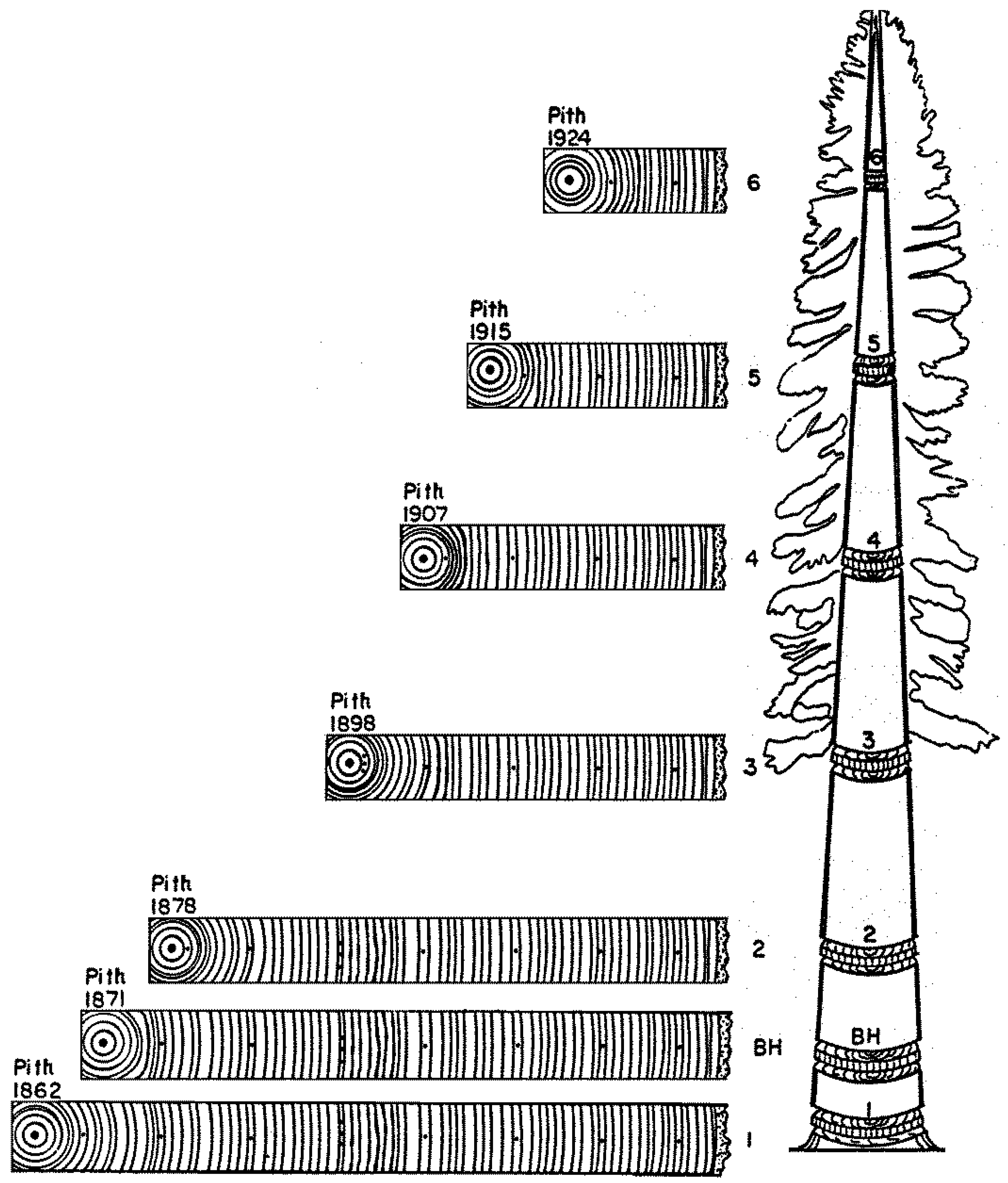
Years ago a figure appeared in a publication on the use of crossdating for stem analysis, i.e., the quantitative description of tree growth at various heights along the trunk. This quintessential dendrochronological application was illustrated by synchronous ring-width patterns from one stem section to another (Figure 1). As it turned out, something was definitely wrong with this picture. Was it the position of each section along the stem? Or the calendar years assigned to the pith? This article is aimed at an audience that cannot immediately recognize the error(s), even though it can distinguish and appreciate the matching sequences of narrow and wide rings depicted in this cartoon.

Before continuing, it is appropriate to review a few definitions and measures. At the macroscopic level, the width (w_t, mm) of each tree ring is equal to the difference between the current stem radius (R_t, cm) and the prior year one (R_t−1, cm). Ring area (a_t, mm ²) is the difference between the area of a circle with radius R_t and the area of a smaller circle with radius R_t−1. When a ring is locally absent, it is given a zero value for width or area, rather than considering it as a missing observation. The number of years from the pith is called cambial age, a value that refers to a tree ring, not to the vascular cambium, whose physiological ability to divide and form new tissue defies the commonly held notions of aging and senescence [9]. Basal area, i.e., the transverse surface of the trunk, is typically calculated from stem diameter at ‘breast height’ (1.3–1.5 m from the ground) measured outside bark. Diameter is converted to area assuming a perfect circle, and radial growth, or basal area increment (BAI), is computed as the difference between consecutive basal areas. Annual BAI is equivalent to ring area, which however can refer to any position along the stem, not just breast height. Ring area is also independent of bark thickness, which changes between species as well as with tree age and size, stem position, and site conditions [10].

In the forestry literature, current annual increment is used to indicate any measure of growth over a year, whereas periodic increment refers to growth over a time interval longer than one year, as in 5- or 10-year periods [11]. Besides calculating increments in a ‘forward’ direction, i.e., from the innermost to the outermost growth layer, annual or periodic basal area increment can also be calculated from measurements of tree diameter outside bark by removing the estimated bark thickness, and then progressively subtracting the ring-width measurements to reconstruct past diameters [12]. Because the tree pith is rarely in the geometric center of the stem, the proportional method proposed by [13] is recommended for reconstructing historical tree diameters. Both the ‘forward’ (i.e., from the pith to the bark) and the ‘backward’ (i.e., from the bark to the pith) calculation of ring areas are available in the dplR software package [14] for the R computing environment [15].

Because tree rings represent radial growth and the increase in stem size over time, they also contribute to describing its ontogeny, i.e., the origin and development of the tree as an organism. Changes in tree size during its life history are often portrayed by cumulative growth curves, where the actual size, rather than its increment, is plotted over time. Because annual growth measures the rate of change in tree size with respect to time, the difference between consecutive increments, such as ring widths (w_t − w_t−1), represents the rate of change in growth increment with respect to time, which is an index of growth acceleration [11]. Authors who favor measures of growth acceleration usually apply a logarithmic transformation beforehand to stabilize the variance of the time series [16], assuming that the relative, rather than the absolute, growth fluctuation is affected by an underlying trend [17] (p. 94). Differencing tree-ring widths or areas results in frequency distributions no longer bound by a minimum value of zero. It also generates values for locally absent rings that are not immediately identifiable because they correspond to growth accelerations with varying non-positive values.

Studies of tree growth have a number of practical applications because of the multiple ways in which wood is utilized, from energy source to construction material. Therefore, a multitude of mathematical formulas, ranging from fully empirical to wholly theoretical, have been proposed to calculate tree volume using stem diameter (hence basal area), height, and taper, which describes how stem diameter changes with height [18]. For convenience and ease of measurement, some of those formulas estimate total tree size using basal stem diameter alone [19]. Additional equations allow the calculation of tree biomass, usually measured as dry weight, and carbon content, which in recent times has become an important variable because of the need to quantify biogeochemical cycles [20].

Another commonly used measure in plant biology is relative growth rate, which takes into consideration how plant growth depends on existing biomass at the start of the growth period, and is therefore a useful tool for evaluating size changes over time in the same organism or over space among different organisms [21]. Relative growth rate was originally expressed as the difference between log-transformed plant weights over a certain time interval [22]. It is expected to decrease monotonically and nonlinearly with increasing plant size and age, eventually approaching zero when photosynthesis and respiration reach a balance. It can also be calculated as a growth percentage when the ratio between increment (ring width, ring area, BAI, or others) and initial size is multiplied by 100 [11]. To avoid confusion, a clear distinction needs to be made between relative growth (RG_t), which is the increment with respect to initial plant size, and relative growth change (RGC_t), which is the increase in size with respect to the previous increment. The following section uses simple equations to clarify the abovementioned concepts, mostly derived from the forestry and plant population biology literature, in terms of dendrochronological measurements.

3. Simple Mathematical Relationships

When considering annual increments, because only one unit of time is considered, relative growth (RG) is the same in terms of either simple interest rates or compound interest rates (see formulas 15-7 and 15-8 in [11] (p. 374). For ring width, or half diameter increment, one can then write:

$$RG{w}_t(\%)=100\frac{w_t}{R_{t-1}}=\frac{100w_t}{{{\displaystyle \sum }}_{i=1}^{i=t-1}{w}_i}.$$

(1)

For ring area, or annual basal area increment, relative growth can still be calculated from ring width, as demonstrated below based on the definition of ring area given in the previous section.

$$\begin{gathered} RG{a}_t(\%)=100\frac{a_t}{\pi R_{t-1}^2}=100\frac{\pi \left[{\left(R_{t-1}+w_t\right)}^2- R_{t-1}^2\right]}{\pi R_{t-1}^2}=100\frac{\left[R_{t-1}^2+w_t^2+2w_t{R}_{t-1}- R_{t-1}^2\right]}{R_{t-1}^2} \\ = 100\frac{w_t^2+2w_t{R}_{t-1}}{R_{t-1}^2}=100\left(\frac{w_t^2}{R_{t-1}^2}+2\frac{w_t}{R_{t-1}}+1-1\right)=100\left[{\left(1+\frac{w_t}{R_{t-1}}\right)}^2-1\right]. \end{gathered}$$

(2)

Using Harper’s [22] original formulation, which was based on natural logarithms (ln), relative radial growth rate (RGR_t) could be expressed as:

$$RG{R}_t=\frac{\ln R_t-\ln R_{t-1}}{t-\left(t-1\right)}=\ln \left(\frac{R_t}{R_{t-1}}\right)=\ln \left(\frac{w_t+R_{t-1}}{R_{t-1}}\right)=\ln \left(1+\frac{w_t}{R_{t-1}}\right).$$

(3)

A more meaningful adaptation of this approach would require comparing increment to the amount of living tissues at the start of the growing period, which is “a virtually impossible task with the tree” [22] (p. 218). A viable alternative is relative growth change (RGC), which is the ratio between the current increment (ring width, ring area, etc.) and the previous one. Because ring-width measurements reach a minimum of zero when a growth layer is locally absent [23], a positive constant k needs to be added to the ring-width or ring-area measurements to avoid dividing by zero. In equation form:

$$RGC{w}_t=\frac{w_t+k}{w_{t-1}+k}\mathrm{and}RGC{a}_t=\frac{a_t+k}{a_{t-1}+k},$$

(4)

with k often defaulted to unity. However, instead of dividing, one can subtract the previous increment from the current one, obtaining a measure of growth acceleration (∆_t). When growth acceleration is computed from log-transformed increments (∆l_t), it becomes a log-transformed relative growth change. This statement can be demonstrated using ring widths, as follows (here the positive constant k needs to first be added to avoid taking the logarithm of zero):

$$\Delta l{w}_t=\ln \left(w_t+k\right)-\ln \left(w_{t-1}+k\right)=\ln \frac{w_t+k}{w_{t-1}+k}.$$

(5)

Another measure that can be derived from ring-width measurements and is based on the concept of relative growth is the percentage growth change [24]. This measure (GC_t) is defined for each year t as the relative difference between two consecutive averages of 10-year ring-width periods, one that ends at year t and another that immediately follows. In mathematical notation, it can be written as:

$$G{C}_t(\%)=100\frac{\frac{{{\displaystyle \sum }}_{i=t+1}^{i=t+10}{w}_i}{10} - \frac{{{\displaystyle \sum }}_{i=t-9}^{i=t}{w}_i}{10}}{\frac{{{\displaystyle \sum }}_{i=t-9}^{i=t}{w}_i}{10}}=100\frac{{{\displaystyle \sum }}_{i=t+1}^{i=t+10}{w}_i - {{\displaystyle \sum }}_{i=t-9}^{i=t}{w}_i}{{{\displaystyle \sum }}_{i=t-9}^{i=t}{w}_i}.$$

(6)

A thorough review of GC and many other methods that have been proposed to quantify sudden changes in ring-width series [25] suggested replacing the average with the median, which is less sensitive to the influence of large values [26]. Using that approach, the percentage growth change, identified as RMED by [25], is then computed as:

$$RME{D}_t(\%)=100\frac{me{d}_{i=t+1}^{i=t+10}{w}_i - me{d}_{i=t-9}^{i=t}{w}_i}{me{d}_{i=t-9}^{i=t}{w}_i}.$$

(7)

The following section provides a simple illustration of these various definitions and concepts.

4. A Visual Example of Tree-Ring Data

A graphical comparison among tree-ring measurements and computed values is provided using a cross-section from a Douglas fir (Pseudotsuga menziesii (Mirb.) Franco) that was part of archaeological excavations conducted at Broken Flute Cave, in northeastern Arizona within the Navajo Nation territory (Figure 2). The growth trend displayed by this sample, from wider rings near the pith to progressively narrower ones towards the bark, is typical of tree species that grow in relative isolation, without heavy competition for resources. (The cross-sections depicted in Figure 1 are characterized by a different growth trend from the pith to the bark, but this is neither right nor wrong—merely plausible. However, counting the rings on each of those sections does reveal incorrect pith dates. That is not the main error though.) The development of modern tree-ring science is rooted in the archaeology of the southwestern United States [27,28], so it is perhaps fitting that an archaeological specimen should introduce the measurements. Using this sample also reverberates the use of MLK ring widths to illustrate how dendrochronological standardization [29,30,31,32] ideally operates—measurements from this collection were used in Figure 1.9 of [23] to show curve-fitting—and even hints at the recurring debates on how volcanic eruptions can (or cannot) be dated using tree-ring records [33].

Image analysis software was used to measure the width of each ring in the MLK sample along a direction perpendicular to the ring boundaries. When dealing with conifer samples, it is also possible to measure width along the lines of tracheids formed during the year, but in this case the image magnification did not allow the identification of individual cells. Calendar dates shown on the specimen were assigned by the original investigators after crossdating its ring patterns against a reference, or master, tree-ring chronology. Rather than calendar year, in this exercise the cambial age was used as the time index. Given the regular shape of the ring boundaries, there was no assessment of measurement error. Measurement variability caused by choosing different radii on a cross section, or different increment cores of the same tree, or different trees from the same species and site, is normally dealt with during the standardization phase [37].

All of the parameters defined in the previous section were computed from the MLK ring-width measurements (Figure 3). Ring width and ring area fluctuated widely over most of the tree lifetime, with ring area showing a less pronounced downward trend than ring width. Growth acceleration, calculated as the difference between consecutive ring widths (∆w) or ring areas (∆a), showed abrupt swings, which can be viewed as a ‘rebound’ effect caused by the presence of isolated narrow rings. A similar effect was also noticeable for relative growth changes (RGCw and RGCa). Such isolated small rings, also called ‘marker’ or ‘pointer’ years [34], can occur in sequence, generating a ‘signature’ [3,38], and are particularly important for crossdating. However, their presence inflates the maxima in first-differenced or first-divided time series, so that the resulting peaks are both conspicuously high and occurring a year later than the original minima in ring widths or ring areas. Using a logarithmic transformation before first differencing (∆lw and ∆la) did not remove the ‘rebound’ effect but made the year-to-year variability slightly more homogenous over time. Growth acceleration values, when employed for tree-ring analysis, are therefore computed as log-transformed relative growth changes [16]. Relative growth rates (RGw, RGa, RGR) were characterized by a very rapid (i.e., in less than five years) initial decrease and then a flattening out to a relatively constant value, as it is expected for this type of growth curve [39]. Given that crossdating is founded and predicated on pattern matching, the lack of year-to-year variability in relative growth rates when compared to ring width or ring area clarifies why the latter two variables are preferred in tree-ring science.

Cumulated rings widths and ring areas subtly portrayed the slower increase over time of basal area compared to stem radius at low cambial ages (<40 years), followed by a reversal as time passed and the stem enlarged (Figure 3). As the trunk expands, its slowly shrinking one-dimensional increments can still translate into not-so-decreasing two-dimensional growth rates. Percentage growth changes (GC and RMED) changed more slowly, i.e., at interdecadal time scales rather than interannual ones, with little difference in fluctuations between running means (GC) or medians (RMED). A growth reduction greater than 50% was calculated for cambial ages 32–33, although visually (from Figure 2) one would have expected the timing to be a few years later (37–38). Running means or medians applied to time-series data can be viewed as linear filters that provide a form of smoothing [40], but their properties, and the way in which peaks, dips, and periodicities differ between the original and the transformed time series, require careful consideration [41,42].

5. From Dendrochronology to Allometry

Growth of organisms is intimately linked with their ability to survive and reproduce, and it determines how shape and size of individuals, communities, and ecosystems change over time and space. Connecting growth patterns with the origin and development of the tree as an organism (ontogeny) and with species-specific evolutionary traits (phylogeny) while accounting for environmental variability should therefore occupy a primary role in tree-ring science. It was Leonardo da Vinci who in the late 1400s made multiple observations on tree rings, from the fact that they can be used for age determination to their relationship with annual climatic regime [37]. It was again in Leonardo’s writings that we find another observation closely related to tree features: “All the branches of trees at every stage of their height, united together, are equal to the thickness of their trunk” [43] (p. 306). This concept was formalized much later in the ‘pipe model theory’ [44], whereby an assemblage of pipes, either actively linking foliage with roots, or no longer being used, determine tree form as well as its growth in both height and diameter [45]. In this framework, a unit of leaf area is supplied by a unit area of conducting tissue in the stem, and the total cross-sectional area of conducting tissue is considered constant at all heights between the crown base and the ground [18].

Echoes of Leonardo’s hypothesis that foreshadowed the pipe model theory had emerged in the mid-nineteenth century, and are referred to as ‘Pressler’s laws’ [46]. One of them, in particular, states that “Ring area growth (cross-sectional area of a single annual increment) at any one point on the stem is proportional to the quantity of foliage above this point” (Pressler 1864 as cited by [46], p. 2). This hypothesis sparked a lively controversy between Pressler and other scientists of his time, involving the way in which radial increment (ring width, ring area, or ring volume) was measured. The distribution of annual growth along the tree stem determines its form, or taper, and Larson [46] outlined potential mechanisms, from nutritional to hydraulic, and from mechanical to hormonal, that could control the allocation of new photosynthate to different tree organs. An effective way to test Pressler’s ‘law’ and similar hypotheses is through stem analysis [47,48], the subject of Figure 1. And in case the reader has not yet found all the dating error(s) in that figure, its corrected version is presented in Figure 4. Tree rings were incorrectly dated in the original cartoon.

To dispel any possible confusion, crossdating can be falsified because it is a testable hypothesis, which has resisted innumerable trials. For the sake of argument, let us assume that Figure 1 were indeed correct. Because it is also assumed that matching sequences of ring widths were formed at the same time, one would have to conclude that (a) new wood growth is formed from the pith outward, and (b) rings near the bark disappear in greater numbers at higher levels. Given our current knowledge of tree physiology and wood formation, both of those conclusions can safely be discarded.

In fact, the message conveyed by Figure 1 is that the same tree-ring pattern occurs in different historical periods at different heights during the tree lifetime. To put it another way, accurate assignment of calendar years to wood increments would not be possible by matching ring-width patterns at different heights along the stem. Notice that indeed ring-width patterns can sometime be erratic and not replicable, for example in relatively young trees located in dense stands or in areas where the separation between growing and dormant season is not pronounced [50]. What is shown in Figure 1, however, is that tree-ring patterns can be replicated, but then the cartoon misinterprets the temporal sequence in which wood growth occurs, causing the assigned dates to be incorrect. As a consequence of erroneous pattern matching, the influence of environmental changes on tree-ring patterns would no longer be detectable. One would incorrectly conclude either that factors internal to the tree are able to control all growth variability, or that environmental influences on year-to-year variability are causing lagged responses with fixed delay intervals at various tree heights. A correct representation of both crossdating and stem analysis is thus provided (Figure 5).

Growth layer profiles [51], which are generated from detailed stem analysis, track changes in radial size or increment along the tree height, sketching the pattern of wood distribution along the bole as the tree grows. These patterns depend on competitive interactions [52], as well as other environmental factors and tree conditions at the time of the increment [53]. For instance, ring area often increases from the tree apex to a point near the crown base, below which it varies less compared to its pronounced increase near the ground [46,54], generating the so-called ‘butt swell’ of tree trunks. With regard to Pressler’s ‘law’, data from stem analysis studies have suggested a nonlinear relationship between ring area at a point and foliage area above that point [55]. Clearly, the accuracy of such investigations and their conclusions rely on assigning exact calendar dates to each growth layer both within and among trees.

Stem analysis data are also at the heart of mathematical expressions that quantify changes over time or space in tree volume and biomass as a function of stem size. The most accurate results can be obtained by estimating the parameters that link stem diameter, tree height and taper in a parsimonious model [11]. Many of these relationships are based on exponential formulas [56], and for some applications, especially those that consider mature trees that no longer increase in height, simplifications are possible. For instance, biomass estimates for tree species in North America have been obtained [57] using:

$$B=exp\left(a+b\ln D\right),$$

(8)

where D is diameter at breast height (cm), B is total aboveground biomass (kg) for trees with D ≥ 2.5 cm, and ln is the natural logarithm. When the exponential function has base e, Euler’s irrational number, using logarithmic scales in what are called log-log plots allows this transformation:

$$\ln B=a+b\ln D,$$

(9)

which describes a straight line in Cartesian space [26]. Similarly, for European tree species, the majority of equations used for estimating biomass (B) have the following form [58]:

$$\log B=a+b\log D,$$

(10)

where log is either the natural or a base 10 logarithm, and D is diameter at breast height, either in cm or in logarithmic units.

Despite the applied nature of these exponential, or power, relationships, they occupy a fundamental role in more theoretical studies. Allometry, or scaling analysis, aims at quantifying how attributes of organisms vary with their size, and scaling rules have been identified between the size of a body part (for either animals or plants) and the total size of the organism without that part [59]. These relationships can be written as a power function, i.e.,

$$Y\propto \beta X^{\alpha },$$

(11)

where $\propto$ indicates a proportional relationship between the predictand Y (for example, annual plant growth) and the predictor X (for example, plant biomass before its annual increment) mediated by the allometric constant β and by the allometric (or scaling) exponent α. The currently prevailing power scaling theory was proposed in the 1990s by West, Brown, and Enquist (or WEB) [60,61,62]. It derives a value for the scaling exponent α of 3/4, or 0.75, based on combinations of quarter-power (1/4 or 0.25) scaling exponents caused by the fractal architecture of internal networks involved in the distribution of resources in all organisms. Values of the allometric constant β can vary widely, and no unifying theory has yet emerged in that regard [63]. Pipe model theory was incorporated in the first incarnation of the WEB power scaling model of allometry. In that framework, total tree leaf mass is considered to scale with stem basal area, or sapwood area when it is considered a fixed percentage of the cross-sectional surface. Because in the classic rigid-pipe model the sum of cross-sectional areas (n) at a higher (daughter) branching level (k) equals that of the lower (parent) one (k − 1), it is possible to express the cross-sectional area of conductive tissue as follows:

$$\pi r_{k-1}^2=n·\pi r_k^2.$$

(12)

From this relationship, one can derive that:

$$r_k^2=\frac{\pi r_{k-1}^2}{n·\pi }=\frac{r_{k-1}^2}{n},$$

(13)

and therefore:

$$r_k=\frac{r_{k-1}}{\sqrt{n}}.$$

(14)

The ‘area-preserving branching relation’ [60] is then given by:

$$\frac{r_k}{r_{k-1}}=\frac{r_{k-1}}{\sqrt{n}}·\frac{1}{r_{k-1}}=\frac{1}{\sqrt{n}}=n^{-0.5},$$

(15)

which is independent of branching level k. This relationship assumes that all conductive tissue in the sapwood, the ‘pipes’, contribute equally to water transport, a notion that does not take into account hydraulic conductance [64]. According to the Hagen-Poiseuille law, flow rate is proportional to the fourth power of capillary diameter (hence radius), which is equivalent to the square of conduit area. This implies a disproportionate effect of conduit size on transport, which is ignored by measures of sapwood area as a whole, and it would require comparisons to be made of the calculated flow rates, rather than stem areas. Even anatomical measures, such as average cell lumen, which are now used in studying climatic influences on wood formation [65,66], underestimate flow rates under the Hagen-Poiseuille law. (It can be shown using elementary algebra that flow rate, when calculated by applying the Hagen-Poiseuille law to the average conduit size, is lower than the value obtained by averaging flow rates computed for each of the conduits. Formulas have been proposed to take this issue into account, e.g., [67].) On the other hand, for most woods, measured conductivity is from 20% to 100% of the theoretical value, a discrepancy that may balance off the use of conduit size to estimate flows, and that in conifers is most likely due to the need for water to go through bordered pits when advancing to the next tracheid [68].

It is worth mentioning that other experimental and observational results do not match the pipe model theory. One of them is the need for longer and longer conduits as the tree grows in height, so that rings of greater cambial age normally incorporate wider and longer conductive cells near the ground in order to compensate for the increased transport distances [68,69]. Furthermore, xylem elements are typically organized in intricate, transversally spiral and tangentially fan-shaped patterns around the stem, with multiple interconnections so that a single root feeds a disproportionately large section of the crown, and a single branch relies on many roots, making the tree overall more resilient to environmental stressors [70]. Simple experiments have demonstrated that sequential cuts along the stem, even when the combined surface of the cuts equals the stem area, may not result in tree death because of the non-straight and non-independent nature of its conductive organs [64]. Genetic differences have been uncovered, as in most haploxylon pines the conduits are spiraling around the stem in a direction which is opposite to the direction found in diploxylon species. Other patterns, from interlocked to zig-zagging to straight, are restricted to some species but not others [71]. The spiral nature of wood is on majestic display in weathered trunks of gnarled high-elevation conifers [72] and is reflected in the narrow scars that often twist around the stem of trees hit by lightning strikes [73]. A comprehensive review of spiral and wave patterns in wood is presented in [74].

Expansions and modifications of the WEB theoretical framework have addressed the shortcomings of the pipe model [61,75]. Tapering of conductive tissue is considered uniform for all conduits and such that hydrodynamic resistance becomes independent of path length [76]. In addition, fluid transport is modeled up to the leaf petiole to avoid within-leaf complications [77], and the exponent in the ‘area-preserving branching relation’ is allowed to vary from the original 1/2 to about 1/3 for seedlings and small plants [78]. Alternative hypotheses exist, such as those that view the tree as a ‘cantilever’, i.e., a structure that is supported at one end (the soil) and carries a load along its length (the weight of the tree itself), so that its growth, shape, and functions are geared towards resisting gravity and wind stress [79].

Even more encompassing than the WEB theory, but intimately related to it, is the metabolic theory of ecology (MTE) [80]. The MTE is based on a power scaling between, on one hand, the rate at which organisms acquire, transform, and utilize energy and materials, and, on the other hand, their body size and temperature. This single scaling constraint is then used to define biological processes from an individual’s physiology up to the functioning of entire ecosystems [81]. Overall, an impressive amount of natural phenomena can be explained by applying WEB and MTE principles [82], although controversies remain about its theoretical foundations and empirical validity [83,84]. Scaling rules found in biological systems, geophysical features (such as river basins), and human products (such as computer technologies or airplanes), have even been unified under a ‘constructal’ theory as classes of designs that evolve by providing greater and greater access to the currents that flow through them [85].

It truly needs to be emphasized that several allometric derivations are of direct interest for tree-ring science, since wood density, tree lifespan, and age to reproduction can be linked by scaling rules [86]. Stem biomass of individual trees is considered proportional to the 8/3 power of basal stem diameter for any size class [87]. If the number of trees in forest ecosystems is related to basal stem diameter by a −2 scaling rule, and the second derivation holds, then tree density and above-ground biomass are linked by a −¾ scaling rule [88]. Given the need for further study [89], one would infer that exactly dated tree rings, and their measurements, are crucial contributors to the testing and betterment of such allometric relationships.

6. Conclusions

As a word of caution, while dendrochronological dates are extremely reliable when sufficient sample replication exists, both numerical and visual confidence in calendar dates inevitably decrease as the sample depth declines, which is most common going further and further back in time. Because inter-laboratory calibration of dating and measuring practices does not formally exist among tree-ring research centers, high-profile dates are corrected by means of scientific debates (e.g., [90]). Occasionally, samples are swapped by teams of individual researchers, but a systematic procedure for resolving possible dating issues has not been considered necessary. It would then be ideal to design a crossdating algorithm that guarantees accurate results even when the analyst does not understand its numerical details, does not realize how it should be applied to a specific research question, or does not fully understand the nature of the wood samples s/he is studying. This hypothetical scenario is far from being realized. Human intervention, and the investigator’s ability to distinguish between default options and appropriate ones, routine vs. special cases, adhering to tradition or braving innovation, remains a requirement for obtaining meaningful results.

Mentioning abstract propositions made by famous scientists in cursory fashion, after similarly brief allusions to applied methods used by many generations of foresters, is intended to provide a window, no matter how small, into fields of research that could benefit by enlisting tree-ring experts, and at the same time are worthy of greater attention among dendrochronologists. My brief foray, and conceptual musings, into the fascinating combination of wood form and function can barely hint at the exquisitely intricate connections between dendrochronology, wood science, tree physiology, forest ecology, mensuration, and allometry.

References

- Dobbertin, M.K.; Grissino-Mayer, H.D. The bibliography of dendrochronology and the glossary of dendrochronology: Two new online tools for tree-ring research. Tree-Ring Res. 2004, 60, 101–104. [Google Scholar]
- Stokes, M.A.; Smiley, T.L. An Introduction to Tree-Ring Dating; Reprint of the 1968 Edition; University of Arizona Press: Tucson, AZ, USA, 1996; p. 73. [Google Scholar]
- Douglass, A.E. Crossdating in dendrochronology. J. For. 1941, 39, 825–831. [Google Scholar]
- Fritts, H.C.; Swetnam, T.W. Dendroecology: A Tool for Evaluating Variations in Past and Present Forest Environments. In Advances in Ecological Research; Begon, M., Fitter, A.H., Ford, E.D., MacFadyen, A., Eds.; Academic Press: San Diego, CA, USA, 1989; Volume 19, pp. 111–188. [Google Scholar]
- Nash, S.E. Time, Trees, and Prehistory: Tree-Ring Dating and the Development of North American Archaeology, 1914–1950; The University of Utah Press: Salt Lake City, UT, USA, 1999; p. 294. [Google Scholar]
- Webb, G.E. Tree Rings and Telescopes: The Scientific Career of A.E. Douglass; The University of Arizona Press: Tucson, AZ, USA, 1983; p. 242. [Google Scholar]
- Studhalter, R.A. Early history of crossdating. Tree-Ring Bull. 1956, 1956, 31–35. [Google Scholar]
- Wimmer, R. Arthur Freiherr von Seckendorff-Gudent and the early history of tree-ring crossdating. Dendrochronologia 2001, 19, 153–158. [Google Scholar]
- Peñuelas, J.; Munné-Bosch, S. Potentially immortal? New Phytol. 2010, 187, 564–567. [Google Scholar] [CrossRef] [PubMed]
- Shmulsky, R.; Jones, P.D. Forest Products and Wood Science: An Introduction, 6th ed.; Wiley-Blackwell: New York, NY, USA, 2011; p. 477. [Google Scholar]
- Husch, B.; Beers, T.W.; Kershaw, J.A., Jr. Forest Mensuration; John Wiley & Sons: Hoboken, NJ, USA, 2003; p. 443. [Google Scholar]
- LeBlanc, D.C. Temporal and spatial variation of oak growth–climate relationships along a pollution gradient in the midwestern United States. Can. J. For. Res. 1993, 23, 772–782. [Google Scholar] [CrossRef]
- Bakker, J.D. A new, proportional method for reconstructing historical tree diameters. Can. J. For. Res. 2005, 35, 2515–2520. [Google Scholar] [CrossRef]
- Bunn, A.G.; Biondi, F. Dendrochronology in R with the dplR library. In Abstracts of WorldDendro2010, The 8th International Conference on Dendrochronology; Mielikäinen, K., Mäkinen, H., Timonen, M., Eds.; METLA: Rovaniemi, Finland, 2010; p. 274. [Google Scholar]
- R Core Team. R: A language and Environment for Statistical Computing, version 3.0.2; R Foundation for Statistical Computing: Vienna, Austria, 2015. [Google Scholar]
- Van Deusen, P.C. A dynamic program for cross-dating tree rings. Can. J. For. Res. 1990, 20, 200–205. [Google Scholar] [CrossRef]
- Box, G.E.P.; Jenkins, G.M. Time Series Analysis: Forecasting and Control; Revised ed.; Holden-Day: Oakland, CA, USA, 1976. [Google Scholar]
- Valentine, H.T.; Mäkelä, A. Bridging process-based and empirical approaches to modeling tree growth. Tree Physiol. 2005, 25, 769–779. [Google Scholar] [CrossRef]
- Van Laar, A.; Akça, A. Forest Mensuration; Springer: Dordrecht, The Netherlands, 2007; Volume 13. [Google Scholar]
- Schlesinger, W.H. Biogeochemistry: An Analysis of Global Change, 2nd ed.; Academic Press: San Diego, CA, USA, 1997. [Google Scholar]
- Paine, C.E.T.; Marthews, T.R.; Vogt, D.R.; Purves, D.; Rees, M.; Hector, A.; Turnbull, L.A. How to fit nonlinear plant growth models and calculate growth rates: An update for ecologists. Methods Ecol. Evol. 2012, 3, 245–256. [Google Scholar] [CrossRef]
- Harper, J.L. Population Biology of Plants; Academic Press: London, UK, 1977; p. 892. [Google Scholar]
- Fritts, H.C. Tree Rings and Climate; Academic Press: London, UK, 1976; p. 567. [Google Scholar]
- Nowacki, G.J.; Abrams, M.D. Radial-growth averaging criteria for reconstructing disturbance histories from presettlement-origin oaks. Ecol. Monogr. 1997, 67, 225–249. [Google Scholar] [CrossRef]
- Rubino, D.L.; McCarthy, B.C. Comparative analysis of dendroecological methods used to assess disturbance events. Dendrochronologia 2004, 21, 97–115. [Google Scholar] [CrossRef]
- Sokal, R.R.; Rohlf, F.J. Biometry, 4th ed.; W.H. Freeman and Co.: New York, NY, USA, 2012; p. 937. [Google Scholar]
- Douglass, A.E. The secret of the Southwest solved by talkative tree rings. Natl. Geogr. Mag. 1929, 736–770. [Google Scholar]
- Nash, S.E. Archaeological tree-ring dating at the millennium. J. Archaeol. Res. 2002, 10, 243–275. [Google Scholar] [CrossRef]
- Biondi, F.; Qeadan, F. A theory-driven approach to tree-ring standardization: Defining the biological trend from expected basal area increment. Tree-Ring Res. 2008, 64, 81–96. [Google Scholar] [CrossRef]
- Helama, S.; Lindholm, M.; Timonen, M.; Eronen, M. Detection of climate signal in dendrochronological data analysis: A comparison of tree-ring standardization methods. Theor. Appl. Climatol. 2004, 79, 239–254. [Google Scholar] [CrossRef]
- Meko, D.M.; Friedman, J.M.; Touchan, R.; Edmondson, J.R.; Griffin, E.R.; Scott, J.A. Alternative standardization approaches to improving streamflow reconstructions with ring-width indices of riparian trees. Holocene 2015, 25, 1093–1101. [Google Scholar] [CrossRef]
- Zhang, X.; Li, J.; Liu, X.; Chen, Z. Improved EEMD-based standardization method for developing long tree-ring chronologies. J. For. Res. 2019. [Google Scholar] [CrossRef]
- Biondi, F. Dendrochronology, Volcanic Eruptions. In Encyclopedia of Scientific Dating Methods; Rink, W.J., Thompson, J.W., Eds.; Springer: Dordrecht, The Netherlands, 2015; pp. 1–11. [Google Scholar] [CrossRef]
- Schweingruber, F.H.; Eckstein, D.; Serre-Bachet, F.; Bräker, O.U. Identification, presentation and interpretation of event years and pointer years in dendrochronology. Dendrochronologia 1990, 8, 9–38. [Google Scholar]
- Baillie, M.G.L. Dendrochronology raises questions about the nature of the AD 536 dust-veil event. Holocene 1994, 4, 212–217. [Google Scholar] [CrossRef]
- Baillie, M.G.L. Tree-ring chronologies present us with independent records of past natural events which, strangely, or perhaps not so strangely, seem to link with some stories from myth. In Kalendarische, Chronologische und Astronomische Aspekte der Vergangenheit; Krojer, F., Starke, R., Eds.; Differenz-Verlag: München, Germany, 2012; pp. 109–129. [Google Scholar]
- Speer, J.H. Fundamentals of Tree-Ring Research; University of Arizona Press: Tuscon, AZ, USA, 2010; p. 333. [Google Scholar]
- Kelly, P.M.; Munro, M.A.R.; Hughes, M.K.; Goodess, C.M. Climate and signature years in west European oaks. Nature 1989, 340, 57–60. [Google Scholar] [CrossRef]
- Minot, C.S. The Problem of Age, Growth, and Death; G.P. Putnam’s Sons, The Knickerbocker Press: New York, NY, USA, 1908; p. 280. [Google Scholar]
- Mallows, C.L. Some theory of nonlinear smoothers. Ann. Stat. 1980, 8, 695–715. [Google Scholar] [CrossRef]
- Slutzky, E. The summation of random causes as the source of cyclic processes. Econometrica 1937, 5, 105–146. [Google Scholar] [CrossRef]
- Owens, A.J. On detrending and smoothing random data. J. Geophys. Res. Space Phys. 1978, 83, 221–224. [Google Scholar] [CrossRef]
- MacCurdy, E. The Notebooks of Leonardo da Vinci; George Braziller: New York, NY, USA, 1955; p. 1247. [Google Scholar]
- Shinozaki, K.; Yoda, K.; Hozumi, K.; Kira, T. A quantitative analysis of plant form: The pipe model theory. I. Basic analyses. Jpn. J. Ecol. 1964, 14, 97–105. [Google Scholar]
- Valentine, H.T. Tree-growth models: Derivations employing the pipe-model theory. J. Theor. Biol. 1985, 117, 579–585. [Google Scholar] [CrossRef]
- Larson, P.R. Stem form development of forest trees. For. Sci. 1963, 9, 1–42. [Google Scholar] [CrossRef]
- LeBlanc, D.C.; Raynal, D.J.; White, E.H. Acidic deposition and tree growth: 1. The use of stem analysis to study historical growth patterns. J. Environ. Qual. 1987, 16, 325–333. [Google Scholar] [CrossRef]
- Speer, J.H.; Holmes, R.L. Effects of pandora moth outbreaks on ponderosa pine wood volume. Tree-Ring Res. 2004, 60, 69–76. [Google Scholar] [CrossRef]
- Vaganov, E.A.; Hughes, M.K.; Shashkin, A.V. Growth Dynamics of Conifer Tree Rings: Images of Past and Future Environments; Springer: New York, NY, USA, 2006; Volume 183, p. 354. [Google Scholar]
- Biondi, F.; Fessenden, J.E. Radiocarbon analysis of Pinus lagunae tree rings: Implications for tropical dendrochronology. Radiocarbon 1999, 41, 241–249. [Google Scholar] [CrossRef]
- Duff, G.H.; Nolan, N.J. Growth and morphogenesis in the Canadian forest species: I. The controls of cambial and apical activity in Pinus resinosa Ait. Can. J. Bot. 1953, 31, 471–513. [Google Scholar] [CrossRef]
- Bevilacqua, E.; Puttock, D.; Blake, T.J.; Burgess, D. Long-term differential stem growth responses in mature eastern white pine following release from competition. Can. J. For. Res. 2005, 35, 511–520. [Google Scholar] [CrossRef]
- Arbaugh, M.J.; Peterson, D.L. Stemwood Production Patterns in Ponderosa Pine: Effects of Stand Dynamics and Other Factors; PSW-RP-217; Pacific Southwest Research Station: Albany, CA, USA, 1993; p. 11.
- Cortini, F.; Groot, A.; Filipescu, C.N. Models of the longitudinal distribution of ring area as a function of tree and stand attributes for four major Canadian conifers. Ann. For. Sci. 2013, 70, 637–648. [Google Scholar] [CrossRef]
- Kershaw, A.; Maguire, A. Influence of vertical foliage structure on the distribution of stem cross-sectional area increment in western hemlock and balsam fir. For. Sci. 2000, 46, 86–94. [Google Scholar]
- Jenkins, J.C.; Chojnacky, D.C.; Heath, L.S.; Birdsey, R.A. National-scale biomass estimators for United States tree species. For. Sci. 2003, 49, 12–35. [Google Scholar]
- Jenkins, J.C.; Chojnacky, D.C.; Heath, L.S.; Birdsey, R.A. Comprehensive Database of Diameter-Based Biomass Regressions for North American Tree Species; Gen. Tech. Rep. NE-319; Northeastern Research Station: Newtown Square, PA, USA, 2004; p. 45. [Google Scholar]
- Zianis, D.; Muukkonen, P.; Mäkipää, R.; Mencuccini, M. Biomass and Stem Volume Equations for Tree Species in Europe; Finnish Society of Forest Science: Helsinki, Finland, 2005; p. 63. [Google Scholar]
- Niklas, K.J. Plant Allometry: The Scaling of Form and Process; The University of Chicago Press: Chicago, IL, USA, 1994; p. 395. [Google Scholar]
- West, G.B.; Brown, J.H.; Enquist, B.J. A general model for the origin of allometric scaling laws in biology. Science 1997, 276, 122–126. [Google Scholar] [CrossRef] [PubMed]
- West, G.B.; Brown, J.H.; Enquist, B.J. A general model for the structure and allometry of plant vascular systems. Nature 1999, 400, 664–667. [Google Scholar] [CrossRef]
- West, G.B.; Brown, J.H.; Enquist, B.J. The Fourth Dimension of Life: Fractal Geometry and Allometric Scaling of Organisms. Science 1999, 284, 1677–1679. [Google Scholar] [CrossRef]
- Niklas, K.J. Plant allometry: Is there a grand unifying theory? Biol. Rev. 2004, 79, 871–889. [Google Scholar] [CrossRef]
- Zimmermann, M.H. Xylem Structure and the Ascent of Sap; Springer: Berlin, Germany, 1983. [Google Scholar]
- Olano, J.M.; Eugenio, M.; García-Cervigón, A.I.; Folch, M.; Rozas, V. Quantitative tracheid anatomy reveals a complex environmental control of wood structure in continental Mediterranean climate. Int. J. Plant Sci. 2012, 173, 137–149. [Google Scholar] [CrossRef]
- Ziaco, E.; Biondi, F. Wood cellular dendroclimatology: A pilot study on bristlecone pine in the southwest US. In Proceedings of the Fall Meeting of the American Geophysical Union, San Francisco, CA, USA, 14–18 December 2015. Abstract GC33B-1276. [Google Scholar]
- Sperry, J.S.; Nichols, K.L.; Sullivan, J.E.M.; Eastlack, S.E. Xylem embolism in ring-porous, diffuse-porous, and coniferous trees of northern Utah and interior Alaska. Ecology 1994, 75, 1736–1752. [Google Scholar] [CrossRef]
- Tyree, M.T.; Ewers, F.W. The hydraulic architecture of trees and other woody plants. New Phytol. 1991, 119, 345–360. [Google Scholar] [CrossRef]
- Anfodillo, T.; Carraro, V.; Carrer, M.; Fior, C.; Rossi, S. Convergent tapering of xylem conduits in different woody species. New Phytol. 2006, 169, 279–290. [Google Scholar] [CrossRef] [PubMed]
- Tyree, M.T.; Zimmermann, M.H. Xylem Structure and the Ascent of Sap, 2nd ed.; Springer: Berlin, Germany, 2002; p. 283. [Google Scholar]
- Rudinsky, J.A.; Vité, J.P. Certain ecological and phylogenetic aspects of the pattern of water conduction in conifers. For. Sci. 1959, 5, 259–266. [Google Scholar]
- Schlenz, M.A.; Flaherty, D. A Day in the Ancient Bristlecone Pine Forest; Companion Press: Bishop, CA, USA, 2008; p. 64. [Google Scholar]
- DeRosa, E.W. Lightning and trees. J. Arboric. 1983, 9, 51–53. [Google Scholar]
- Harris, J.M. Spiral Grain and Wave Phenomena in Wood Formation; Springer: Berlin/Heidelberg, Germany, 1989; p. 214. [Google Scholar]
- Enquist, B.J. Universal scaling in tree and vascular plant allometry: Toward a general quantitative theory linking plant form and function from cells to ecosystems. Tree Physiol. 2002, 22, 1045–1064. [Google Scholar] [CrossRef]
- West, G.B.; Brown, J.H. The origin of allometric scaling laws in biology from genomes to ecosystems: Towards a quantitative unifying theory of biological structure and organization. J. Exp. Biol. 2005, 208, 1575–1592. [Google Scholar] [CrossRef]
- Brown, J.H.; West, G.B.; Enquist, B.J. Yes, West, Brown and Enquist”s model of allometric scaling is both mathematically correct and biologically relevant. Funct. Ecol. 2005, 19, 735–738. [Google Scholar] [CrossRef]
- Enquist, B.J.; Allen, A.P.; Brown, J.H.; Gillooly, J.F.; Kerkhoff, A.J.; Niklas, K.J.; Price, C.A.; West, G.B. Biological scaling: Does the exception prove the rule? Nature 2007, 445, E9–E10. [Google Scholar] [CrossRef]
- Eloy, C. Leonardo’s rule, self-similarity, and wind-induced stresses in trees. Phys. Rev. Lett. 2011, 107, 258101. [Google Scholar] [CrossRef]
- Brown, J.H.; Gillooly, J.F.; Allen, A.P.; Savage, V.M.; West, G.B. Toward a metabolic theory of ecology. Ecology 2004, 85, 1771–1789. [Google Scholar] [CrossRef]
- Price, C.A.; Gilooly, J.F.; Allen, A.P.; Weitz, J.S.; Niklas, K.J. The metabolic theory of ecology: Prospects and challenges for plant biology. New Phytol. 2010, 188, 696–710. [Google Scholar] [CrossRef] [PubMed]
- Whitfield, J. Ecology’s big, hot idea. PLoS Biol. 2004, 2, e440. [Google Scholar] [CrossRef] [PubMed]
- Kozłowski, J.; Konarzewski, M. West, Brown and Enquist’s model of allometric scaling again: The same questions remain. Funct. Ecol. 2005, 19, 739–743. [Google Scholar] [CrossRef]
- Reich, P.B.; Tjoelker, M.G.; Machado, J.-L.; Oleksyn, J. Universal scaling of respiratory metabolism, size and nitrogen in plants. Nature 2006, 439, 457–461. [Google Scholar] [CrossRef] [PubMed]
- Bejan, A.; Lorente, S. The constructal law of design and evolution in nature. Philos. Trans. R. Soc. Lond. B Biol. Sci. 2010, 365, 1335–1347. [Google Scholar] [CrossRef]
- Enquist, B.J.; West, G.B.; Charnov, E.L.; Brown, J.H. Allometric scaling of production and life-history variation in vascular plants. Nature 1999, 401, 907–911. [Google Scholar] [CrossRef]
- Niklas, K.J.; Spatz, H.-C. Growth and hydraulic (not mechanical) constraints govern the scaling of tree height and mass. Proc. Nat. Acad. Sci. USA 2004, 101, 15661–15663. [Google Scholar] [CrossRef]
- Enquist, B.J.; Niklas, K.J. Invariant scaling relations across tree-dominated communities. Nature 2001, 410, 655–660. [Google Scholar] [CrossRef]
- Price, C.A.; Weitz, J.S.; Savage, V.M.; Stegen, J.; Clarke, A.; Coomes, D.A.; Dodds, P.S.; Etienne, R.S.; Kerkhoff, A.J.; McCulloh, K.A.; et al. Testing the metabolic theory of ecology. Ecol. Lett. 2012, 15, 1465–1474. [Google Scholar] [CrossRef]
- Baillie, M.G.L.; Hillam, J.; Briffa, K.R.; Brown, D.M. Re-dating the English art-historical tree-ring chronologies. Nature 1985, 315, 317–319. [Google Scholar] [CrossRef]
Figure 1.
Graphical representation of tree-ring sequences from seven cross sections taken at multiple heights along a conifer trunk. BH = breast height (~1.3–1.5 m from the ground). There are multiple errors in this cartoon, which provide a learning opportunity and are discussed in the text.
Figure 2.
The stem cross-section known as MLK, an acronym derived from the collector’s (Earl H. Morris) last name initial and the field site (Lukachukai Mountains, within the Navajo Nation in northeast Arizona, USA). It is a Douglas-fir (or PSME, shorthand for Pseudotsuga menziesii (Mirb.) Franco) specimen uncovered from the archaeological excavation of Broken Flute Cave (photo © Laboratory of Tree-Ring Research, Tucson, Arizona; courtesy of Rex Adams). Being an archaeological specimen, there is no bark left on the outside; only the wood remains. The shape of the rings is nearly circular, with yellow-colored earlywood and brown-colored latewood forming each annual growth increment. Year 550 is clearly indicated by an arrow pointing at the conventional two-dot symbol, which is used to mark the half-century year. Other visible single-dot symbols mark each decade, and a three-dot symbol marks the century, year 600 in this case. By a twist of chance, calendar decades on this specimen happen to correspond to cambial decades, so for instance year 550 occurs at the cambial age of 30 years. A change in overall color occurs around year 580, from darker (inside; ~55–60 rings) to lighter (outside; ~45–40 rings). Within the overall trend from wider inner rings to narrower outer ones, there are easy-to-spot ‘pointer’ years [34], i.e., 526, 536, and 543. One of these relatively sudden, single-year growth decreases, year 536, is in common with many other trees and sites, possibly because of a global climatic anomaly caused by one or more major volcanic eruptions [35] or by a comet impact [36]. As one would expect, these hypotheses are quite contentious.
Figure 3.
Time series plots of ring-width measurements and computed growth values for the MLK cross-section (Figure 2). The horizontal x-axis, which represents time, has the same length and scale in every plot. The vertical y-axis, which represents growth, has the same length in every plot and covers the range of the plotted variable, hence the vertical scale is not constant among plots. The growth measurement unit is in parentheses except for RGCw and RGCa, which are dimensionless ratios. For ∆lw and ∆la the measurement unit is in brackets because of the need to add a unit constant to avoid taking the logarithm of zero. A vertical dashed red line was drawn to connect values for the same cambial age, and to visualize the one-year shift of the reversed peak generated by using either relative growth changes or first differences compared to ring widths or ring areas. Cumulative growth curves were also plotted from ring widths (radius) and ring areas (basal area). RGCw = relative growth change (width); RGCa = relative growth change (area); ∆w = first difference of ring widths = growth (radial increment) acceleration; ∆a = first difference of ring areas = growth (basal area increment) acceleration; ∆lw = first difference of log-transformed ring widths = log-transformed relative growth change (using radial increment); ∆la = first difference of log-transformed ring areas = log-transformed relative growth change (using basal area increment); RGw = relative growth (width); RGa = relative growth (area); RGR = relative growth rate; GC = percentage growth change (from means); RMED = percentage growth change (from medians).
Figure 4.
A revised version of Figure 1, without dating errors. The ring sequences in each section were redrawn to better illustrate the concept of crossdating. Color lines are used to identify the three-dimensional ordering of growth layers within a tree. The cambial age of a ring is defined as the number of years from the pith. There are three different ordering schemes, or sequences: (a) transverse, or type 1 sequence, where rings of increasing cambial age are formed over time at the same stem height (cross sections BH and 1 through 6); (b) tangential, or type 2 sequence, where rings of the same cambial age are formed over time at increasing stem heights (red lines connect the rings included in one such sequence); (c) oblique, or type 3 sequence, where rings of increasing cambial age are formed in the same year at increasing stem heights (green lines connect the rings that form one of these sequences). These three ordering schemes correspond to different ways in which tree rings are influenced by environmental variability and internal physiological processes [49] (p. 9).
Figure 5.
A correct way to represent both stem analysis and crossdating. The transverse sections are lined up vertically according to calendar years, which were assigned to the rings by visually crossdating their common patterns across samples. Notice that the ring-width sequences are the same as those in Figure 4. Without properly assigning dates to all growth layers, errors can be made in the analysis of tree growth, either for an individual stem or for a forest, and in any calculations related to changes over time in diameter, height, taper, volume, biomass, and carbon content. Lack of temporal control prevents accurate identification of factors that drive wood formation, thus crossdating becomes crucial for any type of tree growth study at interannual and longer time scales.
© 2020 by the author. Licensee MDPI, Basel, Switzerland. This article is an open access article distributed under the terms and conditions of the Creative Commons Attribution (CC BY) license (http://creativecommons.org/licenses/by/4.0/).
Share and Cite
MDPI and ACS Style
Biondi, F. From Dendrochronology to Allometry. Forests 2020, 11, 146. https://doi.org/10.3390/f11020146
AMA Style
Biondi F. From Dendrochronology to Allometry. Forests. 2020; 11(2):146. https://doi.org/10.3390/f11020146
Chicago/Turabian StyleBiondi, Franco. 2020. "From Dendrochronology to Allometry" Forests 11, no. 2: 146. https://doi.org/10.3390/f11020146
APA StyleBiondi, F. (2020). From Dendrochronology to Allometry. Forests, 11(2), 146. https://doi.org/10.3390/f11020146
Note that from the first issue of 2016, this journal uses article numbers instead of page numbers. See further details here.