Abstract
A large area of Estonian hemiboreal forest is recovering from clear-cut harvesting and changing carbon (C) balance of the stands. However, there is a lack of information about C- source/sink relationships during recovery of such stands. The eddy covariance technique was used to estimate C-status through net ecosystem exchange (NEE) of CO2 in two stands of different development stages located in southeast Estonia in 2014. Measured summertime (June–September) mean CO2 concentration was 337.75 ppm with mean NEE −1.72 µmol m−2 s−1. June NEE was −4.60 µmol m−2 s−1; July, August, and September NEE was −1.17, −0.77, and −0.25 µmol m−2 s−1, respectively. The two stands had similar patterns of CO2 exchange; measurement period temperature drove NEE. Our results show that after clear-cutting a 6-year-old forest ecosystem was a light C-sink and 8-year-old young stand demonstrated a stronger C-sink status during the measurement period.
1. Introduction
The important role of forests in the global carbon cycle is through relations between forest characteristics, climate conditions, and ecosystem functioning [1,2], which vary over time and stand age [3,4,5]. Most carbon balance estimations in European forest ecosystems have been measured in middle-aged stands [6], overlooking C-dynamics as stands age.
Disturbances play a key role in ecosystem carbon (C) dynamics [7,8,9]. Natural and anthropogenic disturbances in forest ecosystems significantly affect the C-balance [10,11,12], ecosystem functioning, and stand development [10,13,14,15,16,17]. Forest management, particularly clear-cut harvesting, alters C storage and fluxes, thereby increasing the chance that more carbon dioxide (CO2) will be released into the atmosphere [10,18]. Conversely, photosynthesis in actively growing young forests removes CO2 by uptake [19,20].
After significant stand-replacing disturbances, forest ecosystems generally act as C-sources, releasing more CO2 than plants and soil microorganisms can absorb [19]. Nevertheless, carbon uptake quickly rises as forest biomass recovers with age, becoming C-sinks within about 10 years [7]. Middle-aged managed forests continue acting as C-sinks [6,18,21] until net ecosystem exchange (NEE) with the atmosphere declines with advancing age [4,6,22].
Eddy covariance (EC) is a micrometeorological method favored for estimating C-balance and NEE [9,16,23,24]. EC directly measures fluxes and assesses the carbon exchange of the whole forest ecosystem with the atmosphere above the canopy [9,10,21,23,24]. The widely used EC method provides continuous measurement of carbon fluxes at the stand-level for studies of ecosystem physiology [6,8,23,25].
The main idea of NEE is to quantify C-uptake into ecosystems by taking into account several components of the carbon cycle [26,27]. A negative NEE means the atmosphere is losing carbon, while a positive NEE indicates that the atmosphere is absorbing carbon [5,18,28,29]. Duration and amount of carbon release depends on factors that affect C-stocks, including photosynthesis, vegetation and soil respiration, and weather [6,8,18,19,20,24,30,31]. Forest management affects C-source/sink strength. After clear-cutting, a forest ecosystem becomes a carbon source and usually soil C-storage decreases [6,9]. Using EC, we sought to identify current CO2 levels and to quantify carbon dynamics in terms of C-sink or C-source status in two young stands that developed after clear-cutting. Our hypothesis is that the studied stands performed as weak C-sinks throughout the measurement period (June–September).
2. Materials and Methods
2.1. Site Description
The study site (58°16.890′ N, 27°18.315′ E) was located at the Järvselja Training and Experimental Forest Centre, Estonia, in the hemiboreal forest zone. The site is characterized by a continental climate, with warm summers and severe winters. In Estonia, the coldest month is February and the warmest is July. At the study site during the study period (May to September), monthly mean temperature was lowest in September (11.4 °C) and highest in July (18.5 °C), with a mean temperature of 15 °C. The soils of both stands are gleyic podzols soils and the Oxalis-Vaccinium myrtillus site type [32]. The stands are adjacent and before harvesting had similar growing conditions (Figure 1). Data for this study are from June to September 2014.
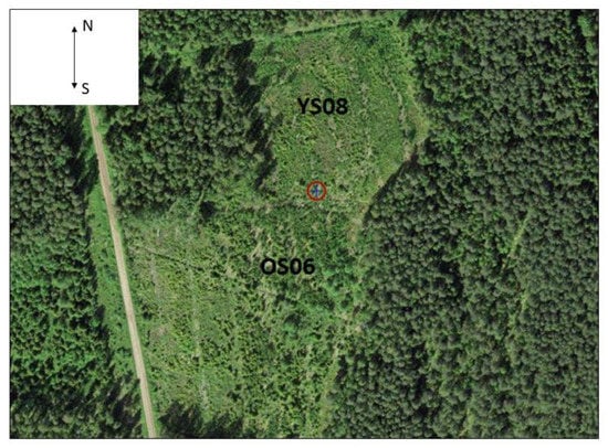
Figure 1.
Location of the eddy flux tower (red circle) and the study stands (YS08, OS06).
The study area was divided into two parts according to harvest year; the younger stand was clear-cut in 2008 (YS08) and the older stand in 2006 (OS06) (Table 1). Before clear-cutting the dominant tree species in YS08 were Scots pine (Pinus sylvestris L.), silver birch (Betula pendula Roth) and Norway spruce (Picea abies (L.) Karst). Scots pine was also the dominant tree species in OS06, but Norway spruce and silver birch were present. Understory vegetation was mainly rough small reed (Calamagrostis arundinacea (L.) Roth), sedges (Carex spp. L.), and lingonberry (Vaccinium vitis-idaea L.). Several years after clear-cutting, the dominant tree species at YS08 were silver birch and Norway spruce, with a minor component of Scots pine. Dominance at OS06 changed to Norway spruce and silver birch, with minor amounts of European aspen (Populus tremula L.) and Scots pine (Table 1).

Table 1.
Characteristics of the stands at the Järvselja Training and Experimental Forest Centre, Estonia.
2.2. EC Measurements
An eddy covariance (EC) system [9,23] collected all data, including concentrations and fluxes of CO2 and H2O, and was installed at the study site in 2013. The EC system consists of a sonic anemometer (C-SAT 3, Campbell Scientific, Logan, UT, USA), and a closed-path infrared gas analyzer LI-7200 (LI-COR Biosciences, Lincoln, NE, USA). Temperature, and 3D wind speed and direction were measured using an anemometer. The instruments were mounted at 6 m above the ground, at the border between the two stands (Figure 1). Measurements for the two stands were differentiated by the intervals of main wind directions (Table 1). When wind direction was between 135 to 285 degrees, then EC was measured for the older stand and when wind direction was from 335 to 50 degrees, then it was younger stand.
The sampling line was 1 m (6 mm i.d.). Continuous high frequency (10 Hz) data, collected at half-hour intervals for calculating turbulent eddy fluxes, were saved automatically by datalogger (Campbell Scientific, USA) [23]. Measurements for this study began in 2014 after mounting and calibration. Data were available from June to September for the study sites. Flux data from the surrounding area (0–100 m) were taken also into account (Grace 2004). Carbon and water vapor fluxes data were converted from raw data to half-hourly mean values of micromole per square meter (µmol m−2 s−1) and millimole per square meter (mmol m−2 s−1). Mean values for days, months, and the entire measurement period were calculated from the processed data. Background information of precipitation levels came from a nearby weather station in the Järvselja Hunting Lodge (1.3 km distant) and used to validate other weather variables.
Net ecosystem CO2 exchange (NEE) (µmol m−2 s−1) was calculated as the sum of the measured eddy flux (Fc) [33] and storage flux (Sc) [15,16,25,29,34] according to the following equations:
where
NEE = Fc + Sc
= gas flow of eddy covariance (µmol m-2 s-1),
= air density
= vertical wind speed
= dry mole fraction, and
where,
Zec = height above ground level of EC measurements
= molar density of dry air
Sc = CO2 molar mixing ratio
2.3. Data Processing and Analysis
Quality assessment and control (QA/QC) included flux corrections and canopy storage calculations. The half-hour-average fluxes of CO2 and water vapor were calculated using the EddyPro v6 software (LI-COR Biosciences, Lincoln, NE, USA). Data processing included raw data filtering and statistical tests, such as drop-outs and spike removals [29,35], block averaging, double rotation, time lag compensation, low and high frequency spectral correction [36]. Spike removals were needed to exceed quality control criteria and to ensure the reliability of high frequency data (10 Hz) [16,24], which may be affected by instrument or power failure [37]. Quality check flagging policy included flux quality flags classes from 1–9 according to the test for steady state conditions and developed turbulence following Foken et al. [38].
Further data processing and analysis was carried out in R-Statistics software. We used the method of Iglewicz and Hoaglin [39] to detect bad values in flux data with threshold value of 3.5. To avoid excluding true measurements we rounded up the allowable data region (200–700 ppm) for CO2 concentration and ±100 µmol m−2 s−1 for CO2 flux. The percentage of usable data after filtering was 89.5%.
Budget sums of forest ecosystem were estimated using the gap-filling method recommended by Jaksic et al. [37], performed as a combination of lookup tables [40] and the Reddy ProcWeb online tool (https://www.bgc-jena.mpg.de/bgi/index.php/Services/REddyProcWeb).
We evaluated the cumulative footprint at the clear-cut area every 30 min according to [41,42]. Measured fluxes were taken into account from 0° to 360°. The footprint area analysis showed that 90% of the cumulative footprint was located at 84.9 m distance as well showing the maximum extension of limits of clear-cut area from the tower. Cumulative footprints of 70%, 50%, 30%, and 10 % originated 31.3, 18.7, 11.7, and 5.3 m from the EC tower, respectively. Less than 1% of fluxes (0.5 m) showed offset from the tower. The footprint area completely covered the study and surrounding areas.
In this study, we examined effects of two binary factors (stand with levels “young” and “old” and light with levels “night” and “day”) and several continuous variables like time (hours), air temperature, water vapor, etc., on NEE. We had no a priori reason to choose any particular parametric form for describing the shape of the relationship between NEE and the explanatory variables. In such cases, generalized additive models (GAMs) are useful. For data smoothing we used mgcv implementation of gam in R, contributed by Wood [43]. We selected the penalized cubic regression splines model for smoothing predictors. To study the effect of binary factors on NEE, one-way and two-way analysis of variance (ANOVA) was used as an option in GAM modelling procedure [43].
3. Results
Forest Ecosystem Carbon Balance
On a daily basis (24 h), the study site acted as a C-sink beginning about 07:00 in the morning and a C-source at night (Figure 2). Daytime average NEE was −3.398 µmol m−2 s−1, varying between −96.793 µmol m−2 s−1 and 83.327 µmol m−2 s−1. Around 20.00 h, NEE turned positive for the nighttime period, staying positive but near to neutral level (average 2.749 µmol m−2 s−1).
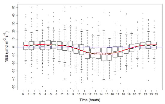
Figure 2.
Values of net ecosystem exchange (NEE, µmol m−2 s−1) over the study period (June to September, 2014) on a 24-h timescale. Red line describes smooth mean of the NEE.
Carbon fluxes were sensitive to temperature and precipitation over the study period. Temperatures stayed above 0 °C and NEE balance was negative (−1.72 µmol m−2 s−1), indicating sink behavior (Figure 3). The beginning of June was cold and wet. Temperatures started rising later in the second half of the month. July was sunny and temperatures (average 18.5 °C) were the highest for the year. NEE showed higher uptake from the atmosphere in June. Fluxes acted as a C-sink between 08:00 and 21:00, between sunrise and sunset. C-uptake started in the mornings one hour after sunrise and respiration dominated in the nighttime one hour after sunset, similarly in every month.
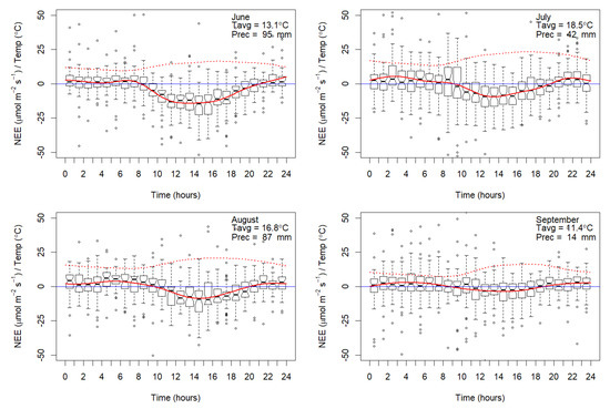
Figure 3.
NEE (µmol m−2 s−1) values per 24-h timescale and precipitation (mm) levels over the study period (June to September 2014). Dark red line describes smooth mean of the NEE, dotted red line illustrates average temperature.
June was the wettest month, followed by August. C-uptake increased with the higher precipitation values. September was sunny with low precipitation and NEE was C-neutral or showed slightly C-negative values.
Highest C-uptake occurred around 20 °C (between 15 to 25 °C) (Figure 4). More limited C-uptake occurred under lower temperature conditions and under extremely high temperatures and drought conditions.
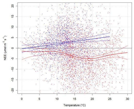
Figure 4.
NEE (µmol m−2 s−1) and temperature (°C) over the study period (2014). Blue dots represent nighttime and red dots daytime eddy flux measurements. Lines represent GAM model predictions with confidence intervals.
The average NEE showed higher C-uptake in the older of the two stands (p-value = 0.001) (Table 2). Average CO2 fluxes differed between nighttime and daytime in every month (Figure 4). The daytime NEE fluxes in the younger YS08 stand averaged −2.187 µmol m−2 s−1 and the average NEE for the older OS08 stand was −4.609 µmol m−2 s−1. However, monthly results were more variable (Table 2). The median fluxes during daytime varied between −0.8913 µmol m−2 s−1 in September and −5.018 µmol m−2 s−1 in June (Figure 5). The sum of daytime average fluxes was −3.492 µmol m−2 s−1.
Table 2.
Average monthly and seasonal values of NEE (µmol m−2 s−1), standard deviations (SD), and data points over the study period.
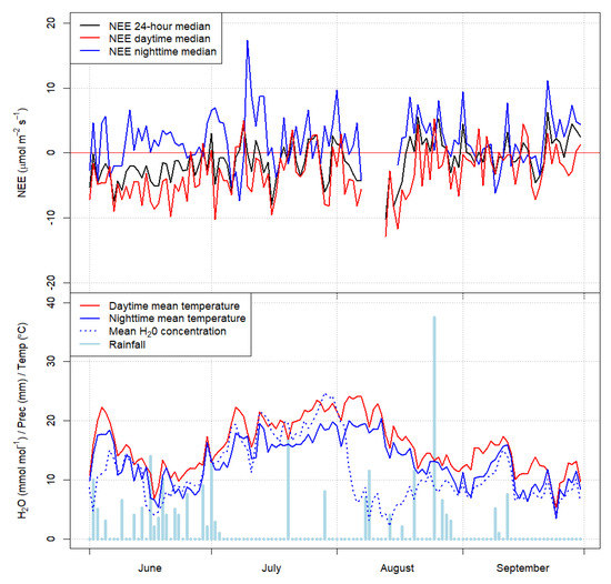
Figure 5.
Daily NEE (µmol m−2 s−1) values; nighttime flux (µmol m−2 s−1), daytime flux (µmol m−2 s−1), NEE average (µmol m−2 s−1), temperature (C°), H2O concentration (mmol mol−1), and rainfall (mm) levels over the study period (2014).
Nighttime NEE fluxes in the younger stand averaged 2.509 µmol m−2 s−1, similar to the older stand (average of 2.989 µmol m−2 s−1). The median nighttime NEE fluxes in June, July, August, and September were 1.238, 2.083, 3.163, and 1.679 µmol m−2 s−1, respectively. The sum of the stands’ nighttime fluxes was 8.163 µmol m−2 s−1 and the monthly average was 2.555 µmol m−2 s−1, peaking in August.
Local wind direction of fluxes generally was from the South, meaning that the wind mainly came from over the OS06 stand. Mean CO2 concentration over YS08 was 339.7 ppm and NEE −0.85 µmol m−2 s−1, however CO2 concentration in the OS06 stand was 335.8 ppm and NEE was −2.22 µmol m−2 s−1. The two stands had similar CO2 concentrations; however, they had different monthly NEE values. Differences in NEE values may be caused by the observed severe summer drought event, resulting in differences in soil moisture conditions, which were moister in OS06 compared to YS08. Due to that, NEE results in July showed concrete differences between OS06 and YS08, where YS08 was a C-source and OS06 a C-sink (Table 2).
4. Discussion
Stand-replacing disturbances have considerable impact on forest ecosystems’ carbon dynamics, often turning ecosystems from C-sinks into C-sources [18,44]. Stands may require several years for recovery to C-sink status [45]. Even-aged management using clear-cutting is common in boreal and temperate forest biomes. This study in Estonia, in the hemiboreal transition between boreal and temperate biomes, presents carbon flux measurements using the eddy covariance technique after a stand-replacing disturbance. The EC method makes reliable and effective measurements of C-fluxes from canopy to atmosphere possible, even in complex terrain [18,25]. EC methods, however, do not provide individual tree flux measurements. Even though this affects dynamical measurements, all analysis and raw data depend more on site-specific conditions [25].
Measurements in two young stands six and eight years after clear-cutting provided estimates of NEE over the measurement period, illustrating monthly, daily, and diurnal variation in source-sink behavior. Over the measurement period (June to September), the two stands were slight C-sinks. In the daytime, the stands were C-sinks, turning to C-source behavior during the nighttime because of the connection with soil respiration, and to a lesser extent, with soil moisture [28,34]. As we hypothesized, the studied stands performed as weak C-sinks during the measurement period. Uri et al. [44] found similar results in a 6-year-old Scots pine stand in Estonia, as did Aguilos et al. [16] with 7-year-old boreal mixed forest stand in Japan. A Canadian jack pine (Pinus banksiana) stand (7 and 8 years old) was almost C-neutral [46]. Taking only the snow free period into account, Payeur-Poirier et al. [47] found C-sink status by an 8-year-old spruce stand. Nevertheless, stands in other locations take longer to become C-sinks, up to 10 to 20 years in other boreal ecosystems [7,16,46,48,49].
Young forests (ages 0 to 10 years) have negative mean rates of net ecosystem production (NEP) because of high heterotrophic respiration [10,46,49,50]. Total ecosystem respiration is high when forests are young [4], but decreases as dead biomass that belonged to the previous forest rotation decomposes [51], although this may not be a monotonic decrease as early theory suggested and certainly depends upon the amount of legacy material left by a disturbance [52]. In boreal forests, it may take decades for NPP to exceed heterotrophic respiration [52,53]. Vigorously growing young stands, however, begin to offset respiration by photosynthetic activity. Temperature differences and variations directly affect both photosynthesis and respiration [17,33,54]. The NEE of forest stands combines the results of these two processes, depending on light, temperature, water vapor, and growing season length [28,49,55].
Photosynthesis and respiration strongly influence daytime NEE, attesting to the important role of photosynthetically active radiation [6,37,44]. Active daytime photosynthesis in our stands was evidenced by higher daytime CO2 concentrations. Daily NEE was C-sink during the daytime and C-source during the night (Figure 5). Other studies in young stands have found similar results, for example, Kolari et al. [6] found nighttime fluxes in a 5-year-old Scots pine stand acting as a C-source (NEE was 3–6 µmol m−2 s−1). During the daytime, the stand acted as a C-sink, but over the study period, the stand was a C-source [6]. Grant et al. [10] showed slight C-sink status on a daily basis from late May to June, similar to Rannik et al. [50] where a clear-cut (five years after disturbance) was a slight C-sink or neutral during the day in the summer.
Over the measurement period, monthly average NEE is sensitive to temperature; fluxes were greatest in June and decreased in September (Table 2). In slightly older logged Eurosiberian stands (7 and 13 years old), Schulze et al. [56] measured daily maximum ecosystem C flux in July between −7 and −4 µmol m−2 s−1. Daytime NEE was close to the compensation point. Similarly, a young (<20 years) planted Norway spruce forest was a C sink; NEE was −10 to −5 g C m−2 d−1 [29]. During the winter season, daily respiration was close to zero so that C-flux was negative.
Carbon budget estimation of our clear-cut areas was −2.076 t C ha−1—definite C-sink status. Despite the short measurement period in our study, our results compare well with other similar locations. Krasnova et al. [57] found annual results for NEE as −5.9 t C ha−1 yr−1. Chi et al. [58] found NEE was 5–8 t C ha−1 yr−1 (500–800 g C m–2 yr−1) six years after clear-cutting, similar to budget estimations in Aguilos et al. [16] and Kolari et al. [6] that found 12-year-old stand C budget is almost neutral.
Extreme precipitation alters CO2 fluxes by influencing C-uptake during very wet conditions [54]. Different weather components, such as tropospheric ozone [59], including clouds [60], excessive rain, or drought, influence ecosystem functioning [17,18,22,54] and all may decrease C-uptake activity. Precipitation events often stimulate respiratory responses of microorganisms. Precipitation and higher humidity also affected C-cycling in our study. Similar results are found in other studies, where precipitation played a key role [5,61]. Wetter weather conditions generally promoted C-uptake (Figure 5). Also some other studies refer to similar results. Oishi et al. [61] found that in very warm and dry conditions, the ecosystem acted more as a weak C-sink, which confirm understanding of the current study. In our conditions, wet and dry weather was varying throughout study period. NEE showed higher uptake of C from the atmosphere in June, even though the temperature was lower at the beginning of the month.
Climate change influences C-cycling by modifying the C-uptake rate and period [7]. Generally, C-balance is sensitive to water availability, which may be important under wetter climate conditions in the future. In addition, drought events may be useful for C-uptake, excepting the extreme drought conditions. On the one hand, the Estonian climate regime may shift to drought conditions, where warmer and drier summers may suppress higher photosynthesis in summertime and cause increases in ecosystem C-uptake [62,63,64] because of the decrease in July to September precipitation [62]. On the other hand, climate may become wetter over large areas of the boreal forest zone, leading to increased mineralization, higher plant productivity, and microbial activity in soils [17,51,65]. In this study, we experienced both warm and wet weather conditions over the summer. In August, there were quite high temperatures and precipitation levels, but low CO2 levels. However, in July the higher peaks in CO2 concentration coincided with average precipitation and high temperature. Some studies have shown that ecosystem respiration may be more variable than photosynthesis [54], thus fluxes may not correlate well with a single factor. Nevertheless, NEE is highly correlated with growing season length. Our results point to the need for greater attention to C-source and sink relationships during early stand development in order to better characterize C-dynamics.
5. Conclusions
Our main question was how much time was needed for recovery from clear-cutting and a return to a functioning ecosystem, in terms of becoming a C-sink. From our study, we can draw four conclusions: (1) Different weather conditions, especially precipitation and temperature, greatly affect forest C-balance; (2) after a stand-replacing disturbance, a 6-year-old forest ecosystem was a light C-sink during the measurement period; (3) an 8-year-old forest ecosystem demonstrated a stronger C-sink status; and (4) both young stands exhibit daytime C uptake and nighttime C losses.
Author Contributions
S.R., K.J., A.K., J.A.S. and M.M. performed the manuscript writing and designed the study. S.R., A.K., M.M. and K.J. analyzed the results. S.R., A.K. produced the figures and tables. S.R. and M.M. led the writing of the manuscript. All authors have read and agreed to the published version of the manuscript.
Funding
This study was supported by the Institutional Research Funding IUT21-4 of the Estonian Ministry of Education and Research, and the project of the Estonian University of Life Sciences P180024MIME.
Acknowledgments
We thank the anonymous reviewers for their valuable comments.
Conflicts of Interest
The authors declare no conflict of interest.
References
- Franklin, J.F.; Spies, T.A.; Pelt, R.V.; Carey, A.B.; Thornburgh, D.A.; Berg, D.R.; Lindenmayer, D.B.; Harmon, M.E.; Keeton, W.S.; Shaw, D.C.; et al. Disturbances and structural development of natural forest ecosystems with silvicultural implications, using Douglas-fir forests as an example. For. Ecol. Manag. 2002, 155, 399–423. [Google Scholar] [CrossRef]
- D’Andrea, E.; Micali, M.; Sicuriello, F.; Cammarano, M.; Ferlan, M.; Skudnik, M.; Mali, B.; Čater, M.; Simončič, P.; Cinti, B.D.; et al. Improving carbon sequestration and stocking as a function of forestry. Ital. J. Agron. 2016, 11, 56–60. [Google Scholar]
- IGBP Terrestrial Carbon Working Group. CLIMATE: The Terrestrial Carbon Cycle: Implications for the Kyoto Protocol. Science 1998, 280, 1393–1394. [Google Scholar] [CrossRef]
- Pregitzer, K.S.; Euskirchen, E.S. Carbon cycling and storage in world forests: Biome patterns related to forest age. Glob. Chang. Biol. 2004, 10, 2052–2077. [Google Scholar] [CrossRef]
- Froelich, N.; Croft, H.; Chen, J.M.; Gonsamo, A.; Staebler, R.M. Trends of carbon fluxes and climate over a mixed temperate–boreal transition forest in southern Ontario, Canada. Agric. For. Meteorol. 2015, 211–212, 72–84. [Google Scholar] [CrossRef]
- Kolari, P.; Pumpanen, J.; Rannik, U.; Ilvesniemi, H.; Hari, P.; Berninger, F. Carbon balance of different aged Scots pine forests in Southern Finland. Glob. Chang. Biol. 2004, 10, 1106–1119. [Google Scholar] [CrossRef]
- Amiro, B.D.; Barr, A.G.; Barr, J.G.; Black, T.A.; Bracho, R.; Brown, M.; Chen, J.; Clark, K.L.; Davis, K.J.; Desai, A.R.; et al. Ecosystem carbon dioxide fluxes after disturbance in forests of North America. J. Geophys. Res. Biogeosci. 2010, 115, G00K02. [Google Scholar] [CrossRef]
- Tang, X.; Li, H.; Ma, M.; Yao, L.; Peichl, M.; Arain, A.; Xu, X.; Goulden, M. How do disturbances and climate effects on carbon and water fluxes differ between multi-aged and even-aged coniferous forests? Sci. Total Environ. 2017, 599–600, 1583–1597. [Google Scholar] [CrossRef]
- Teets, A.; Fraver, S.; Hollinger, D.Y.; Weiskittel, A.R.; Seymour, R.S.; Richardson, A.D. Linking annual tree growth with eddy-flux measures of net ecosystem productivity across twenty years of observation in a mixed conifer forest. Agric. For. Meteorol. 2018, 249, 479–487. [Google Scholar] [CrossRef]
- Grant, R.F.; Barr, A.G.; Black, T.A.; Gaumont-Guay, D.; Iwashita, H.; Kidson, J.; McCAUGHEY, H.; Morgenstern, K.; Murayama, S.; Nesic, Z.; et al. Net ecosystem productivity of boreal jack pine stands regenerating from clearcutting under current and future climates. Glob. Chang. Biol. 2007, 13, 1423–1440. [Google Scholar] [CrossRef]
- Köster, K.; Köster, E.; Orumaa, A.; Parro, K.; Jõgiste, K.; Berninger, F.; Pumpanen, J.; Metslaid, M. How Time since Forest Fire Affects Stand Structure, Soil Physical-Chemical Properties and Soil CO2 Efflux in Hemiboreal Scots Pine Forest Fire Chronosequence? Forests 2016, 7, 201. [Google Scholar] [CrossRef]
- Parro, K.; Koster, K.; Jogiste, K.; Seglins, K.; Sims, A.; Stanturf, J.A.; Metslaid, M. Impact of post-fire management on soil respiration, carbon and nitrogen content in a managed hemiboreal forest. J. Environ. Manag. 2019, 233, 371–377. [Google Scholar] [CrossRef]
- Odum, E.P. An understanding of ecological succession provides a basis for resolving man’s conflict with nature. Sustainability 2005, 164, 9. [Google Scholar]
- Peltzer, D.A.; Bast, M.L.; Wilson, S.D.; Gerry, A.K. Plant diversity and tree responses following contrasting disturbances in boreal forest. For. Ecol. Manag. 2000, 127, 191–203. [Google Scholar] [CrossRef]
- Zha, T.; Barr, A.G.; Black, T.A.; McCaughey, J.H.; Bhatti, J.; Hawthorne, I.; Krishnan, P.; Kidston, J.; Saigusa, N.; Shashkov, A.; et al. Carbon sequestration in boreal jack pine stands following harvesting. Glob. Chang. Biol. 2009, 15, 1475–1487. [Google Scholar] [CrossRef]
- Aguilos, M.; Takagi, K.; Liang, N.; Ueyama, M.; Fukuzawa, K.; Nomura, M.; Kishida, O.; Fukazawa, T.; Takahashi, H.; Kotsuka, C.; et al. Dynamics of ecosystem carbon balance recovering from a clear-cutting in a cool-temperate forest. Agric. For. Meteorol. 2014, 197, 26–39. [Google Scholar] [CrossRef]
- Frank, D.; Reichstein, M.; Bahn, M.; Thonicke, K.; Frank, D.; Mahecha, M.D.; Smith, P.; van der Velde, M.; Vicca, S.; Babst, F.; et al. Effects of climate extremes on the terrestrial carbon cycle: Concepts, processes and potential future impacts. Glob. Chang. Biol. 2015, 21, 2861–2880. [Google Scholar] [CrossRef] [PubMed]
- Baldocchi, D.; Chu, H.; Reichstein, M. Inter-annual variability of net and gross ecosystem carbon fluxes: A review. Agric. For. Meteorol. 2018, 249, 520–533. [Google Scholar] [CrossRef]
- Humphreys, E.R.; Andrew Black, T.; Morgenstern, K.; Li, Z.; Nesic, Z. Net ecosystem production of a Douglas-fir stand for 3 years following clearcut harvesting. Glob. Chang. Biol. 2005, 11, 450–464. [Google Scholar] [CrossRef]
- Tang, J.; Baldocchi, D.D.; Xu, L. Tree photosynthesis modulates soil respiration on a diurnal time scale. Glob. Chang. Biol. 2005, 11, 1298–1304. [Google Scholar] [CrossRef]
- Grace, J. Understanding and managing the global carbon cycle. J. Ecol. 2004, 92, 189–202. [Google Scholar] [CrossRef]
- Wharton, S.; Schroeder, M.; Paw, U.K.T.; Falk, M.; Bible, K. Turbulence considerations for comparing ecosystem exchange over old-growth and clear-cut stands for limited fetch and complex canopy flow conditions. Agric. For. Meteorol. 2009, 149, 1477–1490. [Google Scholar] [CrossRef]
- Baldocchi, D.D. Assessing the eddy covariance technique for evaluating carbon dioxide exchange rates of ecosystems: Past, present and future. Glob. Chang. Biol. 2003, 9, 479–492. [Google Scholar] [CrossRef]
- Yan, J.; Zhang, Y.; Yu, G.; Zhou, G.; Zhang, L.; Li, K.; Tan, Z.; Sha, L. Seasonal and inter-annual variations in net ecosystem exchange of two old-growth forests in southern China. Agric. For. Meteorol. 2013, 182–183, 257–265. [Google Scholar] [CrossRef]
- Nicolini, G.; Aubinet, M.; Feigenwinter, C.; Heinesch, B.; Lindroth, A.; Mamadou, O.; Moderow, U.; Mölder, M.; Montagnani, L.; Rebmann, C.; et al. Impact of CO2 storage flux sampling uncertainty on net ecosystem exchange measured by eddy covariance. Agric. For. Meteorol. 2018, 248, 228–239. [Google Scholar] [CrossRef]
- Carrara, A.; Kowalski, A.S.; Neirynck, J.; Janssens, I.A.; Yuste, J.C.; Ceulemans, R. Net ecosystem CO2 exchange of mixed forest in Belgium over 5 years. Agric. For. Meteorol. 2003, 119, 209–227. [Google Scholar] [CrossRef]
- Sulman, B.N.; Roman, D.T.; Scanlon, T.M.; Wang, L.; Novick, K.A. Comparing methods for partitioning a decade of carbon dioxide and water vapor fluxes in a temperate forest. Agric. For. Meteorol. 2016, 226–227, 229–245. [Google Scholar] [CrossRef]
- Falge, E.; Baldocchi, D.; Olson, R.; Anthoni, P.; Aubinet, M.; Bernhofer, C.; Burba, G.; Ceulemans, R.; Clement, R.; Dolman, H.; et al. Gap filling strategies for defensible annual sums of net ecosystem exchange. Agric. For. Meteorol. 2001, 107, 43–69. [Google Scholar] [CrossRef]
- Jensen, R.; Herbst, M.; Friborg, T. Direct and indirect controls of the interannual variability in atmospheric CO2 exchange of three contrasting ecosystems in Denmark. Agric. For. Meteorol. 2017, 233, 12–31. [Google Scholar] [CrossRef]
- Ilvesniemi, H.; Forsius, M.; Finér, L.; Holmberg, M.; Lepistö, A.; Piirainen, S.; Pumpanen, J.; Rankinen, K.; Starr, M.; Tamminen, P.; et al. Carbon and nitrogen storages and fluxes in Finnish forest ecosystems. Underst. Glob. Syst. 2002, 14, 69–82. [Google Scholar]
- Oren, R.; Hsieh, C.-I.; Stoy, P.; Albertson, J.; Mccarthy, H.R.; Harrell, P.; Katul, G.G. Estimating the uncertainty in annual net ecosystem carbon exchange: Spatial variation in turbulent fluxes and sampling errors in eddy-covariance measurements. Glob. Chang. Biol. 2006, 12, 883–896. [Google Scholar] [CrossRef]
- Lõhmus, E. Eesti Metsakasvukohatüübid; Eesti NSV Metsamajanduse ja Looduskaitse Ministeerium, Eesti NSV Agrotööstuskoondise Info-ja Juurutusvalitsus: Tallinn, Estonia, 1984; pp. 43–44. (In Estonian) [Google Scholar]
- Burba, G.; Madsen, R.; Feese, K. Eddy Covariance Method for CO2 Emission Measurements in CCUS Applications: Principles, Instrumentation and Software. Energy Procedia 2013, 40, 329–336. [Google Scholar] [CrossRef]
- Humphreys, E.R.; Black, T.A.; Morgenstern, K.; Cai, T.; Drewitt, G.B.; Nesic, Z.; Trofymow, J.A. Carbon dioxide fluxes in coastal Douglas-fir stands at different stages of development after clearcut harvesting. Agric. For. Meteorol. 2006, 140, 6–22. [Google Scholar] [CrossRef]
- Vickers, D.; Mahrt, L. Quality Control and Flux Sampling Problems for Tower and Aircraft Data. J. Atmos. Ocean. Technol. 1997, 14, 15. [Google Scholar] [CrossRef]
- Moncrieff, J.; Valentini, R.; Greco, S.; Guenther, S.; Ciccioli, P. Trace gas exchange over terrestrial ecosystems: Methods and perspectives in micrometeorology. J. Exp. Bot. 1997, 48, 1133–1142. [Google Scholar] [CrossRef]
- Jaksic, V.; Kiely, G.; Albertson, J.; Oren, R.; Katul, G.; Leahy, P.; Byrne, K.A. Net ecosystem exchange of grassland in contrasting wet and dry years. Agric. For. Meteorol. 2006, 139, 323–334. [Google Scholar] [CrossRef]
- Foken, T.; Gröockede, M.; Mauder, M. Post-field data quality control. In Handbook of Micrometeorology: A Guide for Surface Flux Measurements and Analysis; Lee, X., Ed.; Kluwer: Dordrecht, The Netherlands, 2004; pp. 181–208. [Google Scholar]
- Iglewicz, B.; Hoaglin, D.C. How to Detect and Handle Outliers; ASQC basic references in quality control; ASQC Quality Press: Milwaukee, WI, USA, 1993; ISBN 978-0-87389-247-6. [Google Scholar]
- Reichstein, M.; Falge, E.; Baldocchi, D.; Papale, D.; Aubinet, M.; Berbigier, P.; Bernhofer, C.; Buchmann, N.; Gilmanov, T.; Granier, A.; et al. On the separation of net ecosystem exchange into assimilation and ecosystem respiration: Review and improved algorithm. Glob. Chang. Biol. 2005, 11, 1424–1439. [Google Scholar] [CrossRef]
- Kljun, N.; Calanca, P.; Rotach, M.W.; Schmid, H.P. A Simple Parameterisation for Flux Footprint Predictions. Bound. Layer Meteorol. 2004, 112, 503–523. [Google Scholar] [CrossRef]
- Kljun, N.; Calanca, P.; Rotach, M.W.; Schmid, H.P. A simple two-dimensional parameterisation for Flux Footprint Prediction (FFP). Geosci. Model Dev. 2015, 8, 3695–3713. [Google Scholar] [CrossRef]
- Wood, S.N. Generalized Additive Models: An Introduction with R.; Texts in statistical science; Chapman & Hall/CRC: Boca Raton, FL, USA, 2006; ISBN 978-1-58488-474-3. [Google Scholar]
- Uri, V.; Kukumägi, M.; Aosaar, J.; Varik, M.; Becker, H.; Aun, K.; Krasnova, A.; Morozov, G.; Ostonen, I.; Mander, Ü.; et al. The carbon balance of a six-year-old Scots pine (Pinus sylvestris L.) ecosystem estimated by different methods. For. Ecol. Manag. 2019, 433, 248–262. [Google Scholar] [CrossRef]
- Chen, B.; Arain, M.A.; Khomik, M.; Trofymow, J.A.; Grant, R.F.; Kurz, W.A.; Yeluripati, J.; Wang, Z. Evaluating the impacts of climate variability and disturbance regimes on the historic carbon budget of a forest landscape. Agric. For. Meteorol. 2013, 180, 265–280. [Google Scholar] [CrossRef]
- Amiro, B.D.; Barr, A.G.; Black, T.A.; Iwashita, H.; Kljun, N.; McCaughey, J.H.; Morgenstern, K.; Murayama, S.; Nesic, Z.; Orchansky, A.L.; et al. Carbon, energy and water fluxes at mature and disturbed forest sites, Saskatchewan, Canada. Agric. For. Meteorol. 2006, 136, 237–251. [Google Scholar] [CrossRef]
- Payeur-Poirier, J.-L.; Coursolle, C.; Margolis, H.A.; Giasson, M.-A. CO2 fluxes of a boreal black spruce chronosequence in eastern North America. Agric. For. Meteorol. 2012, 153, 94–105. [Google Scholar] [CrossRef]
- Coursolle, C.; Giasson, M.-A.; Margolis, H.A.; Bernier, P.Y. Moving towards carbon neutrality: CO2 exchange of a black spruce forest ecosystem during the first 10 years of recovery after harvest. Can. J. For. Res. 2012, 42, 1908–1918. [Google Scholar] [CrossRef]
- Ney, P.; Graf, A.; Bogena, H.; Diekkrueger, B.; Druee, C.; Esser, O.; Heinemann, G.; Klosterhalfen, A.; Pick, K.; Puetz, T.; et al. CO2 fluxes before and after partial deforestation of a Central European spruce forest. Agric. For. Meteorol. 2019, 274, 61–74. [Google Scholar] [CrossRef]
- Rannik, Ü.; Altimir, N.; Raittila, J.; Suni, T.; Gaman, A.; Hussein, T.; Hölttä, T.; Lassila, H.; Latokartano, M.; Lauri, A.; et al. Fluxes of carbon dioxide and water vapour over Scots pine forest and clearing. Agric. For. Meteorol. 2002, 111, 187–202. [Google Scholar] [CrossRef]
- Law, B.E.; Ryan, M.G.; Anthoni, P.M. Seasonal and annual respiration of a ponderosa pine ecosystem. Glob. Chang. Biol. 1999, 5, 169–182. [Google Scholar] [CrossRef]
- Harmon, M.E.; Bond-Lamberty, B.; Tang, J.; Vargas, R. Heterotrophic respiration in disturbed forests: A review with examples from North America. J. Geophys. Res. 2011, 116, G00K04. [Google Scholar] [CrossRef]
- Goulden, M.L.; McMillan, A.M.S.; Winston, G.C.; Rocha, A.V.; Manies, K.L.; Harden, J.W.; Bond-Lamberty, B.P. Patterns of NPP, GPP, respiration, and NEP during boreal forest succession. Glob. Chang. Biol. 2011, 17, 855–871. [Google Scholar] [CrossRef]
- Niu, S.; Fu, Z.; Luo, Y.; Stoy, P.C.; Keenan, T.F.; Poulter, B.; Zhang, L.; Piao, S.; Zhou, X.; Zheng, H.; et al. Interannual variability of ecosystem carbon exchange: From observation to prediction. Glob. Ecol. Biogeogr. 2017, 26, 1225–1237. [Google Scholar] [CrossRef]
- Falge, E.; Baldocchi, D.; Tenhunen, J.; Aubinet, M.; Bakwin, P.; Berbigier, P.; Bernhofer, C.; Burba, G.; Clement, R.; Davis, K.J.; et al. Seasonality of ecosystem respiration and gross primary production as derived from FLUXNET measurements. Agric. For. Meteorol. 2002, 113, 53–74. [Google Scholar] [CrossRef]
- Schulze, E.D.; Lloyd, J.; Kelliher, F.M.; Wirth, C.; Rebmann, C.; Lühker, B.; Mund, M.; Knohl, A.; Milyukova, I.M.; Schulze, W.; et al. Productivity of forests in the Eurosiberian boreal region and their potential to act as a carbon sink-a synthesis. Glob. Chang. Biol. 1999, 5, 703–722. [Google Scholar] [CrossRef]
- Krasnova, A.; Kukumägi, M.; Mander, Ü.; Torga, R.; Krasnov, D.; Noe, S.M.; Ostonen, I.; Püttsepp, Ü.; Killian, H.; Uri, V.; et al. Carbon exchange in a hemiboreal mixed forest in relation to tree species composition. Agric. For. Meteorol. 2019, 275, 11–23. [Google Scholar] [CrossRef]
- Chi, J.; Nilsson, M.B.; Kljun, N.; Wallerman, J.; Fransson, J.E.S.; Laudon, H.; Lundmark, T.; Peichl, M. The carbon balance of a managed boreal landscape measured from a tall tower in northern Sweden. Agric. For. Meteorol. 2019, 274, 29–41. [Google Scholar] [CrossRef]
- Jurán, S.; Edwards-Jonášová, M.; Cudlín, P.; Zapletal, M.; Šigut, L.; Grace, J.; Urban, O. Prediction of ozone effects on net ecosystem production of Norway spruce forest. iForest 2018, 11, 743–750. [Google Scholar] [CrossRef]
- Juráň, S.; Šigut, L.; Holub, P.; Fares, S.; Klem, K.; Grace, J.; Urban, O. Ozone flux and ozone deposition in a mountain spruce forest are modulated by sky conditions. Sci. Total Environ. 2019, 672, 296–304. [Google Scholar] [CrossRef]
- Oishi, A.C.; Miniat, C.F.; Novick, K.A.; Brantley, S.T.; Vose, J.M.; Walker, J.T. Warmer temperatures reduce net carbon uptake, but do not affect water use, in a mature southern Appalachian forest. Agric. For. Meteorol. 2018, 252, 269–282. [Google Scholar] [CrossRef]
- Jaagus, J.; Mändla, K. Climate change scenarios for Estonia based on climate models from the IPCC Fourth Assessment Report. Est. J. Earth Sci. 2014, 63, 166. [Google Scholar] [CrossRef]
- Jaagus, J.; Sepp, M.; Tamm, T.; Järvet, A.; Mõisja, K. Trends and regime shifts in climatic conditions and river runoff in Estonia during 1951–2015. Earth Syst. Dynam. 2017, 8, 963–976. [Google Scholar] [CrossRef]
- Kulmala, L.; Aaltonen, H.; Berninger, F.; Kieloaho, A.-J.; Levula, J.; Bäck, J.; Hari, P.; Kolari, P.; Korhonen, J.F.J.; Kulmala, M.; et al. Changes in biogeochemistry and carbon fluxes in a boreal forest after the clear-cutting and partial burning of slash. Agric. For. Meteorol. 2014, 188, 33–44. [Google Scholar] [CrossRef]
- Johnson, D.W.; Curtis, P.S. Effects of forest management on soil C and N storage: Meta analysis. For. Ecol. Manag. 2001, 140, 227–238. [Google Scholar] [CrossRef]


© 2020 by the authors. Licensee MDPI, Basel, Switzerland. This article is an open access article distributed under the terms and conditions of the Creative Commons Attribution (CC BY) license (http://creativecommons.org/licenses/by/4.0/).