Abstract
Knowledge of forest structure is vital for sustainable forest management decisions. Terrestrial laser scanning cannot describe the canopy trees in a large area, and it is unclear whether unmanned aerial vehicle-light detection and ranging (UAV-LiDAR) data have the ability to capture the forest canopy structural parameters in tropical forests. In this study, we estimated five forest canopy structures (stand density (N), basic area (G), above-ground biomass (AGB), Lorey’s mean height (HL), and under-crown height (hT)) with four modeling algorithms (linear regression (LR), bagged tree (BT), support vector regression (SVR), and random forest (RF)) based on UAV-LiDAR data and 60 sample plot data from tropical forests in Hainan and determined the optimal algorithms for the five canopy structures by comparing the performance of the four algorithms. First, we defined the canopy tree as a tree with a height ≥70% HL. Then, UAV-LiDAR metrics were calculated, and the LiDAR metrics were screened by recursive feature elimination (RFE). Finally, a prediction model of the five forest canopy structural parameters was established by the four algorithms, and the results were compared. The metrics’ screening results show that the most important LiDAR indexes for estimating HL, AGB, and hT are the leaf area index and some height metrics, while the most important indexes for estimating N and G are the kurtosis of heights and the coefficient of variation of height. The relative root mean squared error (rRMSE) of five structure parameters showed the following: when modeling HL, the rRMSEs (10.60%–12.05%) obtained by the four algorithms showed little difference; when N was modeled, BT, RF, and SVR had lower rRMSEs (26.76%–27.44%); when G was modeled, the rRMSEs of RF and SVR (15.37%–15.87%) were lower; when hT was modeled, BT, RF, and SVR had lower rRMSEs (10.24%–11.07%); when AGB was modeled, RF had the lowest rRMSE (26.75%). Our results will help facilitate choosing LiDAR indexes and modeling algorithms for tropical forest resource inventories.
1. Introduction
Tropical rainforests are among the largest terrestrial carbon reservoirs and also have the richest biodiversity, which is very important to maintain the global carbon cycle [1,2]. In recent decades, due to the incorrect management of forest resources, the global tropical forest area has decreased dramatically, so carrying out a forest resource attribute inventory is urgently required [3]. The forest structure consists of a canopy, sub-canopy, shrubs, and herbs. While the attributes associated with forests are well-documented [4,5,6], comparatively less is known about the canopy. The canopy consists of many structural elements, such as dominant, co-dominant, and sub-dominant elements, occupying most of the forest resources and affecting the survival and development of the sub-canopy [7], as well as maintaining the biodiversity of the forest ecosystem [8].
Most related articles [9,10,11] have studied forests with different vertical structures as a whole and ignored the different functions of the forests with different vertical structures. For example, Nilsson et al. [12] found that the development and composition of the sub-canopy is a key driver of forest succession dynamics and that canopy trees are likely related to light absorption [13]. In addition, the simple vertical structures of forests in some study areas [9,10,11] limit the study of canopy forests. Therefore, tropical forests with high biodiversity provide us with an opportunity to understand canopy trees.
Some recent studies [14,15,16] have found that canopy trees can affect the coverage of herbaceous layer species, litter decomposition, the soil microbial community structure, etc. When Rosier et al. [14] studied the relationship between the canopy structure and soil microbial community structure, they found that forest canopy structures are capable of affecting the soil microbial community structure. When studying the relationship between the forest canopy and light absorption, Atkins et al. [13] found that the canopy structure index (canopy height and gap fraction) is related to light absorption. In addition, the forest canopy structural parameters (e.g., stand density, basic area, under-crown height, aboveground biomass, etc.) provide a great deal of information on the spatial and temporal distribution of canopy forests, as well as their structural properties, and are considered critical components of a forest inventory [17,18]. Therefore, obtaining spatially continuous estimates of these canopy forest structural parameters will contribute to the sustainable management of tropical forests [19].
It is not easy to understand the canopy structural parameters in tropical forests, as the traditional forest sample plot survey method is time consuming and costly [20,21]. With the rapid development of remote sensing technologies, light detection and ranging (LiDAR) data, as a type of active remote sensing data, have proven to be highly suitable for forest inventory applications, as they are known to be efficient for predicting and mapping a broad range of forest attributes [22]. Recent studies [23,24] in coniferous forests have shown that airborne laser scanning (ALS) can be used to characterize the forest structure. In tropical forests, 10 point/m2 ALS data may not be able to accurately depict the forest canopy structure or even obtain an accurate digital elevation model (DEM). With the development of unmanned aerial vehicle (UAV) technology, a recent study [25] used structure from motion (SfM) to obtain canopy structural features. UAV-SfM only captures the surface structure of the forest, not the interior of the canopy. Therefore, this technology needs to be combined with LiDAR data to achieve the desired results.
Recent advances in hardware and software have integrated LiDAR sensors with UAVs. UAV-LiDAR has received considerable attention in both commercial projects and the research community due to its safety and high point density. UAV-LiDAR data, in the form of a point cloud, can obtain high-precision forest canopy and terrain height information; thus, providing reliable data for large-scale forest attribute surveys and serving as the main source of data in operational forest inventories in many countries and regions. Some studies [6,26,27] have applied UAV-LiDAR to the estimation of forest structure parameters. In tropical forest areas with complex forest canopy structures, whether this technology can obtain the structure of the forest canopy has not yet been determined.
In forest structural parameter modeling, in addition to the selection of remote sensing data sources, another critical step is to identify an appropriate algorithm to establish the forest structural parameter estimation models [28], as the regression model can affect the prediction accuracy of the forest parameters to some extent. As a result that it is relatively simple and offers good performance, linear regression (LR) is often used in forest structural parameter estimation for different ecosystems, such as subtropical, tropical, and temperate forests [29,30,31]. LR methods are based on the linear relationships of forest structural parameters with independent variables and thus may not provide satisfactory results due to the complex relationships between forest structural parameters and remote sensing variables. In this case, some machine learning algorithms, such as support vector regression (SVR), bagged tree (BT), and random forest (RF), can deal with nonlinear relationships. As a consequence, these algorithms have gained increasing attention in the past decade and have been widely employed in forest structural parameter estimation [32,33].
Apart from identifying appropriate regression algorithms, an equally important step is the selection of the most informative independent set of metrics for forest structural parameter estimation. Guyon et al. [34,35] showed that recursive feature elimination (RFE) can maximize model performance. RFE not only reduces the complexity of the model but also avoids over-fitting and improves generalization efficiency. Selecting a small number of metrics generally facilitates the interpretation of the models and their inversion and applicability in a wide range of contexts.
Based on this factor, the present study established 60 30 m × 30 m square plots in the tropical forests of Hainan Province, China. The ability of UAV-LiDAR data to predict canopy forest structural parameters in tropical forests was studied. We also discussed the fitting accuracy of the structural parameters of canopy forests under different regression algorithms. To achieve this goal, we used RFE to screen the LiDAR metrics and used four regression algorithms (LR, RF, BT, and SVR) to model the structural parameters of the five canopy forests.
2. Materials and Methods
2.1. Study Area
This study was conducted in the rainforests of Hainan Island in China (108°46’–110°04’ E, 18°23’–19°11′ N). This area consists of two national forest parks: the Hainan Diaoloshan National Forest Park (DLS) and Hainan Bawangling National Forest Park (BWL) (Figure 1). Hainan Island receives an average annual rainfall of about 1870–2760 mm throughout the year and has a mean annual temperature of 20.8 °C. The vegetation type of BWL is broad-leaved forest, and the most abundant tree species are Ilex kobuskiana, Xanthophyllum hainanense, and Illicium ternstroemioides. The vegetation type of DLS is theropencedrymion, and the most abundant tree species are Dacrydium pierrei, Podocarpus imbricatus, Pentaphylax euryoides, and Alniphyllum fortune.
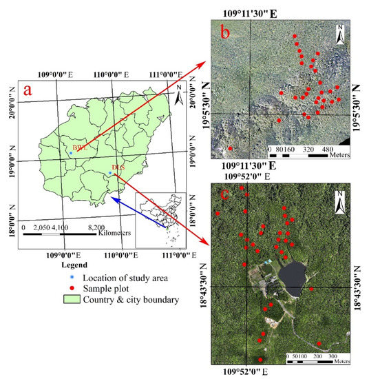
Figure 1.
Figure (a) shows distribution of the studied sites in Hainan Province, figure (b) shows the distribution of Hainan Bawangling National Forest Park (BWL) sample plot, figure c shows the distribution of Hainan Diaoloshan National Forest Park (DLS) sample plot.
2.2. Ground Plot Data
2.2.1. Stand Measurements
The field campaigns were conducted in April 2018. There were 60 sample plots in total, of which 29 plots were located in the BWL, and 31 plots were located in the DSL. All plots were square in shape and 900 m2 in size. Within each plot, the tree diameter at breast height (DBH), under-crown height (hT), and tree height (H) were measured for all trees with a DBH ≥ 5 cm, and the species of each tree was also recorded. The DBH was assessed using the DBH scale, and the H was assessed with a Laser Vertex hypsometer. More detailed statistics of the sites are provided in Table 1. The plot coordinates were measured using a real-time kinematic global navigation satellite system (RTK-GNSS) based on Qianxun continuously operating reference station (CORS) network. As the first commercial BeiDou ground-based augmentation system (GBAS) in China, the Qianxun CORS network announced on May 2016 is able to provide high-precision positioning services for users via the mobile or internet network in most territories in China and can replace RTK base stations during measurements. Huang et al. [36] evaluated an RTK-GNSS based on Qianxun CORS network positioning performance in Wuhan and Chongqing in China. The results showed that the positioning precision can reach the centimeter level for RTK. As a result of the high stand density of tropical rain forests, this type of RTK-GNSS based on Qianxun CORS network positioning performance is affected to a degree, but it can still reach sub-meter accuracy.

Table 1.
Summary of the field measurements.
2.2.2. Canopy Structural Class Definitions
The canopy layer is defined as the highest layer in the vertical structure of the forest [37]. Canopy height is variable according to site quality and stand age and, therefore, needs to be defined at the individual stand level based on relative metrics as opposed to a predetermined height.
To establish an accurate canopy layer, Lorey’s mean height [38] (HL) (Equation (1)) was used:
where h is the measured tree height, and d is the basal area. We defined the canopy tree as the tree with a height of ≥70% HL. Several studies [39,40] have used HL to describe canopy trees because HL can be in any unusual stand structure.
Using our ground height and DBH measurements, the HL was calculated for each plot and applied to the dominant definition. This definition incorporates the height and basal area, giving more weight to trees with a larger DBH, which are more likely to be part of the canopy. After establishing which trees represented the canopy, five variables were calculated from the canopy tree data, including the stand density (N), basic area (G), HL, above-ground biomass (AGB), and hT (Table 2). The individual tree level of the AGB value was calculated using the biomass allometric equations [41,42].
Table 2.
Forest structural parameters of the canopy tree descriptions of the study sites and sample plots.
2.3. UAV-LiDAR Data Acquisition and Pre-Processing
In April 2018, we collected LiDAR data using the UAV-LiDAR system provided by GreenValley. The UAV model was a GV2000, and the laser radar sensor model was an LiAir1000. The flight speed was 4.8 m/s, the pulse repetition frequency was 380 kHz, and the flight altitude was 300 m above ground. The LiDAR sensor wavelength was 1550 nm, the laser divergence was 0.5 mrad, the laser pulse length was 3 ns, and the vertical accuracy was 0.15 m. Finally, due to the limitations of the terrain conditions, the average point density was approximately 72 points/m2.
After the UAV-LiDAR survey, we first input the original inertial measurement unit (IMU) data and base station data into the Inertial Explorer 8.50 software and obtained a smoothed best estimate of the trajectory (SBET) as post-processed position orientation system (POS) data. We then added the post-processed POS data and the original point cloud to the Li-Acquire2 software to obtain the calculated LiDAR data. Secondly, the calculated LiDAR data and the post-processed POS data were added to LiDAR360 4.0 for point cloud data strip matching.
We pre-processed LiDAR data in LiDAR360 4.0 software (GreenValley, Bejing, China). Firstly, we used the built-in algorithm of the LiDAR360 4.0 software (GreenValley, Bejing, China) to remove the floating noise points. Secondly, the point clouds were classified as ground or non-ground points. Then, the Kriging interpolation method [43] was used to generate a digital terrain model (DTM) with a spatial resolution of 1 m. Finally, we subtracted the DTM model from the point cloud data to obtain the normalized point cloud data (Figure 2).
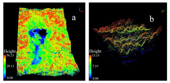
Figure 2.
(a) The normalized three-dimensional point cloud image of DLS, and (b) the three-dimensional structure map of a certain place in DLS.
2.4. UAV-LiDAR-Derived Metrics
Several LiDAR metrics have been proposed as potential predictors of forest structural parameters, such as G and AGB [23,37,44]. Here, we tested a variety of area-based LiDAR metrics (Table 3) related to height distribution (height statistics such as percentiles, mean, median, and standard deviation), intensity metrics, canopy cover, and the leaf area index. For the calculations of features, we excluded the points less than 2 m from the ground because these points are not related to the canopy structure. Finally, a total of 40 LiDAR metrics were calculated (Table 3).
Table 3.
Metrics calculated from light detection and ranging (LiDAR) data and their corresponding abbreviations.
2.5. Regression Models
Four regression algorithms [30,31,45,46,47] were selected in this study (Table 4), encompassing three main approaches: (1) linear models (LR), (2) tree-based models (BT, RF), and (3) kernel-based models (SVR). Four regression algorithms were implemented in the R package caret [48], and the packages required for each algorithm are listed in Table 4. We present an overview of each model below.
Table 4.
Descriptions of the regression models used in this study.
2.5.1. Linear Models
The linear model (LM) is a parametric method that considers the linear relationships between prediction factors and responses. As a result of its simplification and relatively good performance, the LR is often used in forest structural parameter estimation. As a parametric technique, it requires assumptions of linearity, uniformity, and independence [49]. In addition, due to multicollinearity, traditional LM may generate false results.
2.5.2. Tree-Based Models
The foundation of bagging is to build a classifier on each bootstrap sample generated from the learning sample and combine the classifiers to obtain an aggregated predictor. As a result of its strong generalization ability, this method is very useful to reduce the variance of the model [50]. As an improved version of the bagging algorithm, RF combines predictions (by averaging) of multiple classification and regression trees (CART) and is thus more robust to errors and outliers [51]. RF is mainly affected by two parameters, the number of features (mtry) and the number of trees (ntree). In this study, mtry was defined as one-third of the total number of features, and ntree was 1000. As a result of its promising predictive capabilities for high-dimensional datasets, RF has been widely used in remote sensing applications.
2.5.3. Kernel-Based Models
As one of the most effective machine learning techniques, SVR has become an important approach for forest structural parameter modeling in the past decade. The main idea of SVR is to use the kernel function to map the input data to a high-dimensional feature space and transform a nonlinear regression into a linear regression. Choosing the right kernel function can often provide better regression analysis results. The radial basis function (RBF) usually offers better performance than linear and polynomial kernels [31,32]. In this study, we use the RBF for regression prediction.
2.6. Feature Selection
For feature selection, we applied the RFE algorithm, and five canopy structural parameters of each plot were used as the response variables. Using RFE, we assess the effect of the number of input features over the model performance. The performance was evaluated by the root mean squared error (RMSE), quantified in a 5-fold cross-validation scheme and repeated 10 times [34,35]. Through backward selection, all features were first added to the building model, and then their performance (such as error and prediction accuracy) was calculated. Next, the important values of the features were sorted. After deleting the features with the lowest evaluation of this feature, the remaining feature subset modeling was used for iteration and reordering. In this process, the lowest score was deleted until the current remaining feature set was empty. At the end of the process, the number of input features when RMSE was the lowest was selected as the optimal feature subset size.
2.7. Model Validation
In this study, the 10-fold cross validation method was used to train the regression model and verify the model’s accuracy. The accuracy of the different regression models was evaluated by the RMSE and relative root mean squared error (rRMSE) using the following equations (Equation (2), Equation (3)):
where n is the number of plots, is the estimated valued of the forest structural parameters in the sample plot, is the field measured value, and is the mean value field measured parameter.
3. Results
3.1. Selection of LiDAR to Estimate the Canopy Structural Parameters
LM is a regression method whose accuracy is mainly affected by the number of input variables. After reaching optimal accuracy, the RMSE increases (Figure 3). In LM, with an increase in the input variables, except for the under-crown height, the RMSEs of the other models become larger. When LM is used to model the under-crown height, the RMSE value increases with an increase in the input variables after reaching the minimum RMSE value. Considering the limitations of LM on high-dimensional data, this situation is within our expectations. The results of modeling the five forest parameters with BT, RF, and SVR showed that the RMSE value did not increase with an increase in the input variables, so BT, RF, and SVR were less affected by the number of input variables.
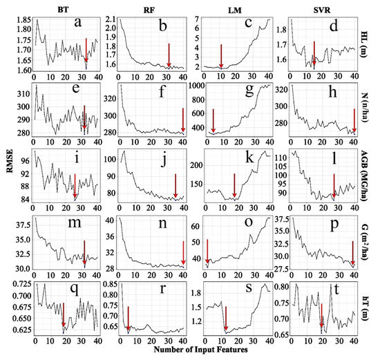
Figure 3.
Effect of the subset feature size on the cross-validated root mean squared error recursive feature elimination (RMSERFE) for the forest structural parameters of canopy trees.
The important LiDAR indexes used to estimate the five forest canopy structure parameters are generally consistent between the models of different regression methods (Figure 4). In addition to some height indicators, canopy structure indicators (such as leaf area index (LAI)) usually contain important information in the model. The most important indexes used to estimate HL and AGB are LAI and some height indexes. The most important indexes for estimating N and G are the height index (H), which can reflect a change in the stand structure (kurtosis of heights (H_KURP), coefficient of variation of height (H_CV)). The index with the largest amount of information to estimate hT is the height index (H_25th, H_50th, H_75th).
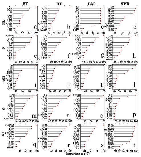
Figure 4.
Relative importance of the 15 highest ranked variables for each regression method with the forest structural parameters of canopy trees. The abbreviations of the LiDAR metrics are given in Table 3.
3.2. Accuracy Assessment of the Canopy Structural Parameters
Figure 5 shows each regression result for the forest structural parameters of the canopy trees, and the accuracy of the UAV-LiDAR data in modeling the canopy structure parameters of the different forests shows great differences (Table 5). The estimation accuracy of N (rRMSE between 26.76% and 29.79%) and AGB (rRMSE between 26.75% and 37.03%) was low, while HL (rRMSE between 10.60% and 12.05%) and hT (rRMSE between 10.24% and 14.27%) had the highest accuracy. AGB was greatly affected by the algorithm. The performance of the LM algorithm was the worst, as it had the lowest accuracy when modeling the five forest canopy structure parameters. The RF algorithms were the most stable, allowing them to produce better results no matter what forest canopy structure parameter was modeled. When modeling HL, the four algorithms showed little difference in accuracy. When N was modeled, BT (rRMSE = 26.76%), RF (rRMSE = 27.21%), and SVR (rRMSE = 27.44%) had high accuracy. For AGB modeling, only the RF (rRMSE = 26.75%) algorithm was the best. In G modeling, the RF (rRMSE = 15.37%) and SVR (rRMSE = 15.87%) performed better. When hT was modeled, BT (rRMSE = 11.07%), RF (rRMSE = 10.34%), and SVR (rRMSE = 10.24%) performed better.
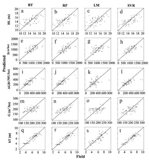
Figure 5.
Each regression result for the forest structural parameters of the canopy trees.
Table 5.
Summary of the regression model statistics.
4. Discussion
4.1. Important Values of the LiDAR Indexes for Estimating Forest Canopy Structure Parameters
Our study confirms the reliability of LiDAR data in predicting the canopy structure parameters of tropical forests, which is consistent with previous tropical studies using ALS LiDAR [4,9,52]. The LiDAR indexes selected here for estimating canopy structure parameters can also be compared with the LiDAR indexes used in other studies [53,54], such as the height percentile and LAI.
In our study, we found that the most important LiDAR indexes used to estimate forest canopy structure parameters are generally consistent in different regression models, which is consistent with the study results of Almeida et al. [34]. For example, the LAI of the four regression models has the highest importance value. When the same regression model is used to predict different forest canopy structure parameters, the input variables in different models are different, which is reasonable. Previous studies [53,55] have shown that different indexes are used to estimate the canopy structure parameters of different forests. The indexes used to estimate HL are usually related to the height percentile characteristics in the LiDAR data. In the estimation of AGB, in addition to some height characteristics, the variables (LAI and coverage closure (CC)) used to reflect the canopy density of the forest also have high importance values. Our study also showed that the LAI in almost all models has a high importance value when used to estimate the canopy structure parameters of five forest species. In a high-density tropical forest, the height differences between stands are not significant, so improving the calculation accuracy of the LAI may be more helpful for estimating the forest canopy structure parameters. In the analysis of hT, the four regression methods showed that the tree height percentile has a high importance value, which was mainly caused by the tree canopy depth, and the lowest branch of the tree was mainly distributed between 25% and 75% of the tree height [56]. In addition, when estimating N and G, it was found that some indexes (H_KURT, H_CV) had a high importance value, which was mainly due to the correlation between stand complexity and stand density [24]. The stand density directly determines the sum of the basal area of the breast height per unit area, which may be an important reason for the similarities of the indexes with higher importance values when modeling N and G.
4.2. Comparison of the Model Accuracy of Different Forest Canopy Structure Parameters
Although many studies [9,32,54] have applied machine learning methods to forest biomass estimation, few studies have applied different machine learning methods to a variety of forest canopy structure parameters. The stand density, HL, under-crown height, and basal area of the breast height are equally important for forest resource management. Fassnacht [57] verified that the RF model is better than other regression models (k-nearest neighbor and stepwise linear regression) when estimating biomass using LiDAR data. In addition, two recent studies [34,58] compared RF with other regression algorithms, and the results showed that RF is more effective in biomass predictions, which is consistent with the results of this study. When RF is used to model the other four forest parameters, higher accuracy can also be obtained, which benefits from the excellent performance of the RF algorithm. Our research found that SVR performs well except for G modeling. In addition, when modeling HL and hT, the accuracy of the SVR algorithm is slightly higher than that of the RF algorithm. Previous studies [46,47] have shown that SVR can perform better even in the case of a small sample size. The BT algorithm also performs well in HL, N, and hT modeling. As an improved version of the BT algorithm, except for the modeling of N, the rRMSE values obtained by the RF algorithm are lower than those obtained by the BT algorithm, which is basically consistent with our expected results. The BT algorithm achieved the best model accuracy when modeling N. Our results also show that LM provides the lowest accuracy compared to the other three machine learning models. The main reason for this low accuracy is that LM, as a parameter algorithm, cannot make full use of all information in the face of high-dimensional characteristics. In addition, our study shows that LM is susceptible to several input characteristics. The performance of the three machine learning algorithms is better than that of the linear model when modeling the five canopy forest parameters. In addition, the RF algorithm shows the most stable effect, but different algorithms are needed to obtain the best model accuracy for different forest canopy structure parameters.
Compared with other studies [53,55,59,60], except for HL, the accuracy of the other forest parameters was slightly higher than the results obtained for other sites. In part, we attribute this accuracy to the optimal characteristic set with the RFE algorithm. In addition, UAV-LiDAR has a higher point density than ALS and may be better able to capture the forest canopy’s structural features. By comparing the accuracy of the five canopy forest parameters in this study, HL (rRMSE = 10.64%) and hT (rRMSE = 10.34%) were shown to have the highest accuracy, which is consistent with the results of other studies [24,61] on the extraction of different forest parameters. LiDAR data were more sensitive to the height characteristics of forest trees. The accuracy of HL obtained in this study was relatively low, likely because in tropical forests with high canopy density, fewer LiDAR point clouds reach the ground, which leads to large DEM errors, and the complex terrain conditions also increase the ability of the LiDAR data to describe the height of the tree crown. In addition, broad-leaved tree species tend to increase the number of LiDAR point clouds reaching the ground [62,63]. When estimating forest parameters with remote sensing data, researchers often ignore the under-crown height. The under-crown height can reflect the height of the canopy and is related to the biomass of individual plants [17]. The results of this study show that UAV-LiDAR data can be used to estimate the average under-crown height (rRMSE = 10.34%), which can successfully estimate forest parameters. Compared to the research results of Noordermeer et al. [19], the accuracy of the N prediction in our study is higher, possibly because, compared to ALS data, high-density UAV-LiDAR data can achieve more abundant canopy structure information. When modeling N, the indicators reflecting the changes in the canopy structure have higher importance values, which indirectly proves this point. The DBH estimation mainly depends on the strong correlation between tree height and DBH [64]. The DBH estimation accuracy directly depends on the extraction accuracy of the tree height, which is the main reason why the accuracy of estimating G is slightly lower than that of HL. In this study, the accuracy of AGB estimation is the lowest, and the appropriate allometric growth equation affects the accuracy of AGB estimation. Fortunately, even though we failed to find the allometric growth equations for all tree species in the study site, we obtained satisfactory results by using different algorithms in modeling (rRMSE = 26.75%).
To summarize, there are many factors affecting the estimation accuracy of forest canopy structure parameters, and the advantages and disadvantages of the algorithms themselves are the main reason. Applying an appropriate remote sensing data source is also an important factor affecting the accuracy of the model [34,65]. In addition, there are some challenges in the simulation of forest parameters in Hainan, such as determining how to obtain high-quality sample site survey data. For example, the site size may be a source of uncertainty in data analysis [58,66]. Especially in tropical forests, where small sites are more vulnerable to boundary effects and global positioning system (GPS) positioning errors [66].
5. Conclusions
This study explored the possibility of estimating the canopy structure parameters of tropical forests using UAV-LiDAR data. In addition, the four regression methods of LR, SVR, BT, and RF were studied and compared. Our conclusions are as follows:
(1) The most important LiDAR indexes used to estimate HL, AGB, and hT are related to LAI and some height characteristics, while the most important indexes for estimating N and G are height indexes, which can reflect changes in the stand structure.
(2) When estimating HL, all four regression models can be used; when estimating N and BT, only RF and SVR should be used; when estimating AGB, only RF should be used; when estimating G, only RF and SVR should be used; BT, RF, and SVR are needed to estimate hT.
Considering the living conditions of tropical forests around the world, it is necessary to engage in a reasonable investigation of forest resources. This study may help forestry departments to quickly and accurately grasp forest canopy structure information and assist those departments in formulating more reasonable tropical forest management measures.
Author Contributions
Conceptualization, Y.C. and Q.C.; data curation, Q.C. and H.L. (Haodong Liu); formal analysis, X.P. and A.Z.; funding acquisition, Q.C.; investigation, Y.C., Q.C., H.L. (Haodong Liu), J.W., and H.L. (Huayu Li); methodology, X.P. and Q.C.; writing—original draft, X.P.; writing—review and editing, Y.C. and Q.C. All authors have read and agreed to the published version of the manuscript.
Funding
This research was funded by the fundamental research funds for the Central Nonprofit Research Institution of Chinese Academy of Forestry (CAF) (grant no. CAFBB2017ZB004), balance funds of Research Institute of Forest Resource Information Techniques (IFRIT), CAF, “Research on the Mechanism of Natural Regeneration barriers of Dacrydium pierrei in Hainan Island” (grant no. 2019JYZJ01).
Acknowledgments
We thank Liyong Fu, Qiuwang Liu, Guangyu Zhu, Jiazheng Liu, Qingqing Yang, and Yihui Chen et al. for assisting in the field work. We thank the support of Diaoluo Natural Reserve of Hainan Island, Hainan Province, China for the experiments.
Conflicts of Interest
The authors declare no conflict of interest.
References
- Huston, M.A.; Marland, G. Carbon management and biodiversity. J. Environ. Manag. 2003, 67, 77–86. [Google Scholar] [CrossRef]
- Saatchi, S.; Marlier, M.; Chazdon, R.L.; Clark, D.B.; Russell, A.E. Impact of spatial variability of tropical forest structure on radar estimation of aboveground biomass. Remote Sens. Environ. 2011, 115, 2836–2849. [Google Scholar] [CrossRef]
- Houghton, R.A. Aboveground Forest Biomass and the Global Carbon Balance. Glob. Chang. Biol. 2005, 11, 945–958. [Google Scholar] [CrossRef]
- Phua, M.-H.; Johari, S.A.; Wong, O.C.; Ioki, K.; Mahali, M.; Nilus, R.; Coomes, D.A.; Maycock, C.R.; Hashim, M. Synergistic use of Landsat 8 OLI image and airborne LiDAR data for above-ground biomass estimation in tropical lowland rainforests. For. Ecol. Manag. 2017, 406, 163–171. [Google Scholar] [CrossRef]
- Iizuka, K.; Yonehara, T.; Itoh, M.; Kosugi, Y. Estimating Tree Height and Diameter at Breast Height (DBH) from Digital Surface Models and Orthophotos Obtained with an Unmanned Aerial System for a Japanese Cypress (Chamaecyparis obtusa) Forest. Remote Sens. 2017, 10, 13. [Google Scholar] [CrossRef]
- Giannetti, F.; Puletti, N.; Puliti, S.; Travaglini, D.; Chirici, G. Assessment of UAV photogrammetric DTM-independent variables for modelling and mapping forest structural indices in mixed temperate forests. Ecol. Indic. 2020, 117, 106513. [Google Scholar] [CrossRef]
- Rissanen, K.A.; Martin-Guay, M.-O.; Riopel-Bouvier, A.-S.; Paquette, A. Light interception in experimental forests affected by tree diversity and structural complexity of dominant canopy. Agric. For. Meteorol. 2019, 278, 107655. [Google Scholar] [CrossRef]
- Draper, F.C.; Asner, G.P.; Coronado, E.H.; Baker, T.R.; García-Villacorta, R.; Pitman, N.C.A.; Fine, P.V.A.; Phillips, O.L.; Gómez, R.Z.; Guerra, C.A.A.; et al. Dominant tree species drive beta diversity patterns in western Amazonia. Ecology 2019, 100, e02636. [Google Scholar] [CrossRef]
- Ferraz, A.; Saatchi, S.S.; Mallet, C.; Jacquemoud, S.; Gonçalves, G.; Silva, C.A.; Soares, P.; Tomé, M.; Pereira, L.G. Airborne Lidar Estimation of Aboveground Forest Biomass in the Absence of Field Inventory. Remote Sens. 2016, 8, 653. [Google Scholar] [CrossRef]
- Frazer, G.; Magnussen, S.; Wulder, M.A.; Niemann, K.O. Simulated impact of sample plot size and co-registration error on the accuracy and uncertainty of LiDAR-derived estimates of forest stand biomass. Remote Sens. Environ. 2011, 115, 636–649. [Google Scholar] [CrossRef]
- Urbazaev, M.; Thiel, C.; Cremer, F.; Dubayah, R.; Migliavacca, M.; Reichstein, M.; Schmullius, C. Estimation of forest aboveground biomass and uncertainties by integration of field measurements, airborne LiDAR, and SAR and optical satellite data in Mexico. Carbon Balance Manag. 2018, 13, 1–20. [Google Scholar] [CrossRef] [PubMed]
- Nilsson, M.; Wardle, D.A. Understory vegetation as a forest ecosystem driver: Evidence from the northern Swedish boreal forest. Front. Ecol. 2005, 3, 421–428. [Google Scholar] [CrossRef]
- Atkins, J.W.; Fahey, R.T.; Hardiman, B.H.; Gough, C.M. Forest Canopy Structural Complexity and Light Absorption Relationships at the Subcontinental Scale. J. Geophys. Res. Biogeosci. 2018, 123, 1387–1405. [Google Scholar] [CrossRef]
- Rosier, C.L.; Van Stan, J.; Moore, L.D.; Schrom, J.O.S.; Wu, T.; Reichard, J.S.; Kan, J. Forest canopy structural controls over throughfall affect soil microbial community structure in an epiphyte-laden maritime oak stand. Ecohydrology 2015, 8, 1459–1470. [Google Scholar] [CrossRef]
- Wallace, K.J.; Laughlin, D.; Clarkson, B.D.; Schipper, L.A. Forest canopy restoration has indirect effects on litter decomposition and no effect on denitrification. Ecosphere 2018, 9, 02534. [Google Scholar] [CrossRef]
- Gilliam, F.S. Response of herbaceous layer species to canopy and soil variables in a central Appalachian hardwood forest ecosystem. Plant Ecol. 2019, 220, 1131–1138. [Google Scholar] [CrossRef]
- Goodman, R.C.; Phillips, O.L.; Baker, T.R. The importance of crown dimensions to improve tropical tree biomass estimates. Ecol. Appl. 2014, 24, 680–698. [Google Scholar] [CrossRef]
- Miura, N.; Jones, S. Characterizing forest ecological structure using pulse types and heights of airborne laser scanning. Remote Sens. Environ. 2010, 114, 1069–1076. [Google Scholar] [CrossRef]
- Pasher, J.; King, D.J. Multivariate forest structure modelling and mapping using high resolution airborne imagery and topographic information. Remote Sens. Environ. 2010, 114, 1718–1732. [Google Scholar] [CrossRef]
- Hermosilla, T.; Ruiz, L.A.; Kazakova, A.N.; Coops, N.C.; Moskal, L.M. Estimation of forest structure and canopy fuel parameters from small-footprint full-waveform LiDAR data. Int. J. Wildland Fire 2014, 23, 224–233. [Google Scholar] [CrossRef]
- Van Leeuwen, M.; Nieuwenhuis, M. Retrieval of forest structural parameters using LiDAR remote sensing. Eur. J. For. Res. 2010, 129, 749–770. [Google Scholar] [CrossRef]
- Vega, C.; St-Onge, B. Mapping site index and age by linking a time series of canopy height models with growth curves. For. Ecol. Manag. 2009, 257, 951–959. [Google Scholar] [CrossRef]
- Goodbody, T.R.; Tompalski, P.; Coops, N.C.; Hopkinson, C.; Treitz, P.M.; Van Ewijk, K. Forest Inventory and Diversity Attribute Modelling Using Structural and Intensity Metrics from Multi-Spectral Airborne Laser Scanning Data. Remote Sens. 2020, 12, 2109. [Google Scholar] [CrossRef]
- Noordermeer, L.; Bollandsås, O.M.; Ørka, H.O.; Næsset, E.; Gobakken, T. Comparing the accuracies of forest attributes predicted from airborne laser scanning and digital aerial photogrammetry in operational forest inventories. Remote Sens. Environ. 2019, 226, 26–37. [Google Scholar] [CrossRef]
- Jayathunga, S.; Owari, T.; Tsuyuki, S.; Hirata, Y. Potential of UAV photogrammetry for characterization of forest canopy structure in uneven-aged mixed conifer–broadleaf forests. Int. J. Remote Sens. 2019, 41, 53–73. [Google Scholar] [CrossRef]
- Shao, G.; Shao, G.; Gallion, J.; Saunders, M.R.; Frankenberger, J.R.; Fei, S. Improving Lidar-based aboveground biomass estimation of temperate hardwood forests with varying site productivity. Remote Sens. Environ. 2018, 204, 872–882. [Google Scholar] [CrossRef]
- Liu, K.; Shen, X.; Cao, L.; Wang, G.; Cao, F. Estimating forest structural attributes using UAV-LiDAR data in Ginkgo plantations. ISPRS J. Photogramm. Remote Sens. 2018, 146, 465–482. [Google Scholar] [CrossRef]
- Lu, D.; Chen, Q.; Wang, G.; Liu, L.; Li, G.; Moran, E.F. A survey of remote sensing-based aboveground biomass estimation methods in forest ecosystems. Int. J. Digit. Earth 2016, 9, 63–105. [Google Scholar] [CrossRef]
- Zhao, P.; Lu, D.; Wang, G.; Wu, C.; Huang, Y.; Yu, S. Examining Spectral Reflectance Saturation in Landsat Imagery and Corresponding Solutions to Improve Forest Aboveground Biomass Estimation. Remote Sens. 2016, 8, 469. [Google Scholar] [CrossRef]
- Zhao, P.; Lu, D.; Wang, G.; Liu, L.; Li, D.; Zhu, J.; Yu, S. Forest aboveground biomass estimation in Zhejiang Province using the integration of Landsat TM and ALOS PALSAR data. Int. J. Appl. Earth Obs. Geoinfor. 2016, 53, 1–15. [Google Scholar] [CrossRef]
- Feng, Y.; Lu, D.; Chen, Q.; Keller, M.; Moran, E.F.; Dos-Santos, M.; Bolfe, É.L.; Batistella, M. Examining effective use of data sources and modeling algorithms for improving biomass estimation in a moist tropical forest of the Brazilian Amazon. Int. J. Digit. Earth 2017, 50, 1–21. [Google Scholar] [CrossRef]
- Gao, Y.; Lu, D.; Li, G.; Wang, G.; Chen, Q.; Liu, L.; Li, D. Comparative Analysis of Modeling Algorithms for Forest Aboveground Biomass Estimation in a Subtropical Region. Remote Sens. 2018, 10, 627. [Google Scholar] [CrossRef]
- Saatchi, S.S.; Malhi, Y.; Zutta, B.; Buermann, W.; Anderson, L.O.; Araujo, A.M.; Phillips, O.L.; Peacock, J.; Ter Steege, H.; Gonzalez, G.L.; et al. Mapping landscape scale variations of forest structure, biomass, and productivity in Amazonia. Biogeosci. Discuss. 2009, 6, 5461–5505. [Google Scholar] [CrossRef]
- De Almeida, C.T.; Galvão, L.S.; Aragão, L.E.D.O.C.E.; Ometto, J.P.H.B.; Jacon, A.D.; Pereira, F.R.D.S.; Sato, L.Y.; Lopes, A.P.; Graça, P.M.L.D.A.; Silva, C.V.D.J.; et al. Combining LiDAR and hyperspectral data for aboveground biomass modeling in the Brazilian Amazon using different regression algorithms. Remote Sens. Environ. 2019, 232, 111323. [Google Scholar] [CrossRef]
- Guyon, I.; Weston, J.; Barnhill, S.; Vapnik, V. Gene Selection for Cancer Classification using Support Vector Machines. Mach. Learn. 2002, 46, 389–422. [Google Scholar] [CrossRef]
- Huang, Y.; Shi, J.; Ouyang, C.; Lu, X. Real-time Observation Decoding and Positioning Analysis Based on Qianxun BeiDou Ground Based Augmentation System. Bull. Surv. Mapp. 2017, 9, 11–14. (In Chinese) [Google Scholar] [CrossRef]
- Jarron, L.R.; Coops, N.C.; MacKenzie, W.H.; Tompalski, P.; Dykstra, P. Detection of sub-canopy forest structure using airborne LiDAR. Remote Sens. Environ. 2020, 244, 111770. [Google Scholar] [CrossRef]
- Næsset, E. Predicting forest stand characteristics with airborne scanning laser using a practical two-stage procedure and field data. Remote Sens. Environ. 2002, 80, 88–99. [Google Scholar] [CrossRef]
- Hyyppa, J.; Kelle, O.; Lehikoinen, M.; Inkinen, M. A segmentation-based method to retrieve stem volume estimates from 3-D tree height models produced by laser scanners. IEEE Trans. Geosci. Remote Sens. 2001, 39, 969–975. [Google Scholar] [CrossRef]
- Maltamo, M.; Eerikäinen, K.; Packalén, P.; Hyyppä, J. Estimation of stem volume using laser scanning-based canopy height metrics. Forestry 2006, 79, 217–229. [Google Scholar] [CrossRef]
- Li, D.; Luo, S.; Lin, M.; Sun, Y. Study on Biomass and Net Primary Productivity of Podocarpus imbricatus Plantation in Jianfengling, Hainan Island. For. Res. 2004, 17, 598–604. (In Chinese) [Google Scholar]
- Li, Y. Comparative analysis of biomass estimation methods for tropical montane rain forest in Hainan Island. Acta Ecol. Sin. 1993, 13, 25–32. (In Chinese) [Google Scholar]
- Oliver, M.A.; Webster, R. Kriging: A method of interpolation for geographical information systems. Int. J. Geogr. Inf. Syst. 1990, 4, 313–332. [Google Scholar] [CrossRef]
- Zhang, Z.; Cao, L.; She, G. Estimating Forest Structural Parameters Using Canopy Metrics Derived from Airborne LiDAR Data in Subtropical Forests. Remote Sens. 2017, 9, 940. [Google Scholar] [CrossRef]
- Cao, L.; Pan, J.; Li, R.; Li, J.; Li, Z. Integrating Airborne LiDAR and Optical Data to Estimate Forest Aboveground Biomass in Arid and Semi-Arid Regions of China. Remote Sens. 2018, 10, 532. [Google Scholar] [CrossRef]
- Gleason, C.J.; Im, J. Forest biomass estimation from airborne LiDAR data using machine learning approaches. Remote Sens. Environ. 2012, 125, 80–91. [Google Scholar] [CrossRef]
- Li, M.; Im, J.; Quackenbush, L.J.; Liu, T. Forest Biomass and Carbon Stock Quantification Using Airborne LiDAR Data: A Case Study Over Huntington Wildlife Forest in the Adirondack Park. IEEE J. Sel. Top. Appl. Earth Obs. Remote Sens. 2014, 7, 3143–3156. [Google Scholar] [CrossRef]
- Kuhn, M. Building Predictive Models in R Using the caret Package. J. Stat. Softw. 2008, 28, 1–26. [Google Scholar] [CrossRef]
- Osbourne, J.W.; Waters, E. Four assumptions of multiple regression that researchers should always test. Pract. Assess. Res. Eval. 2002, 8, 2. [Google Scholar]
- Breiman, L. Bagging Predictors. Mach. Learn. 1996, 24, 123–140. [Google Scholar] [CrossRef]
- Breiman, L. Random Forest. Mach. Learn. 2001, 45, 5–32. [Google Scholar] [CrossRef]
- Lu, J.; Wang, H.; Qin, S.; Cao, L.; Pu, R.; Li, G.; Sun, J. Estimation of aboveground biomass of Robinia pseudoacacia forest in the Yellow River Delta based on UAV and Backpack LiDAR point clouds. Int. J. Appl. Earth Obs. Geoinf. 2020, 86, 102014. [Google Scholar] [CrossRef]
- Cao, L.; Liu, K.; Shen, X.; Wu, X.; Liu, H. Estimation of Forest Structural Parameters Using UAV-LiDAR Data and a Process-Based Model in Ginkgo Planted Forests. IEEE J. Sel. Top. Appl. Earth Obs. Remote Sens. 2019, 12, 4175–4190. [Google Scholar] [CrossRef]
- Wang, D.; Wan, B.; Liu, J.; Su, Y.; Guo, Q.; Qiu, P.; Wu, X. Estimating aboveground biomass of the mangrove forests on northeast Hainan Island in China using an upscaling method from field plots, UAV-LiDAR data and Sentinel-2 imagery. Int. J. Appl. Earth Obs. Geoinf. 2020, 85, 101986. [Google Scholar] [CrossRef]
- Puliti, S.; Ørka, H.O.; Gobakken, T.; Næsset, E. Inventory of Small Forest Areas Using an Unmanned Aerial System. Remote Sens. 2015, 7, 9632–9654. [Google Scholar] [CrossRef]
- Kruger, L.M.; Midgley, J.J.; Cowling, R. Resprouters vs reseeders in South African forest trees; a model based on forest canopy height. Funct. Ecol. 1997, 11, 101–105. [Google Scholar] [CrossRef]
- Fassnacht, F.E.; Hartig, F.; Latifi, H.; Berger, C.; Hernandez, J.; Corvalan, P.; Koch, B. Importance of sample size, data type and prediction method for remote sensing-based estimations of aboveground forest biomass. Remote Sens. Environ. 2014, 154, 102–114. [Google Scholar] [CrossRef]
- Vafaei, S.; Soosani, J.; Adeli, K.; Fadaei, H.; Naghavi, H.; Pham, T.D.; Bui, D.T. Improving Accuracy Estimation of Forest Aboveground Biomass Based on Incorporation of ALOS-2 PALSAR-2 and Sentinel-2A Imagery and Machine Learning: A Case Study of the Hyrcanian Forest Area (Iran). Remote Sens. 2018, 10, 172. [Google Scholar] [CrossRef]
- Xie, B.; Cao, C.; Xu, M.; Bashir, B.; Singh, R.P.; Huang, Z.; Lin, X. Regional Forest Volume Estimation by Expanding LiDAR Samples Using Multi-Sensor Satellite Data. Remote Sens. 2020, 12, 360. [Google Scholar] [CrossRef]
- Bouvier, M.; Durrieu, S.; Fournier, R.A.; Renaud, J.-P. Generalizing predictive models of forest inventory attributes using an area-based approach with airborne LiDAR data. Remote Sens. Environ. 2015, 156, 322–334. [Google Scholar] [CrossRef]
- Valbuena, R.; Hernando, A.; Manzanera, J.-A.; Martínez-Falero, E.; García-Abril, A.; Mola-Yudego, B. Most similar neighbor imputation of forest attributes using metrics derived from combined airborne LIDAR and multispectral sensors. Int. J. Digit. Earth 2017, 11, 1–14. [Google Scholar] [CrossRef]
- Rennie, J.C. Comparison of Height-Measurement Techniques in a Dense Loblolly Pine Plantation. South. J. Appl. For. 1979, 3, 146–148. [Google Scholar] [CrossRef]
- Mielcarek, M.; Stereńczak, K.; Khosravipour, A. Testing and evaluating different LiDAR-derived canopy height model generation methods for tree height estimation. Int. J. Appl. Earth Obs. Geoinfor. 2018, 71, 132–143. [Google Scholar] [CrossRef]
- Panagiotidis, D.; Abdollahnejad, A.; Surový, P.; Chiteculo, V. Determining tree height and crown diameter from high-resolution UAV imagery. Int. J. Remote Sens. 2017, 38, 2392–2410. [Google Scholar] [CrossRef]
- Latifi, H.; Fassnacht, F.E.; Koch, B. Forest structure modeling with combined airborne hyperspectral and LiDAR data. Remote Sens. Environ. 2012, 121, 10–25. [Google Scholar] [CrossRef]
- Mauya, E.W.; Hansen, E.H.; Gobakken, T.; Bollandsås, O.-M.; Malimbwi, R.; Næsset, E. Effects of field plot size on prediction accuracy of aboveground biomass in airborne laser scanning-assisted inventories in tropical rain forests of Tanzania. Carbon Balance Manag. 2015, 10, 1–14. [Google Scholar] [CrossRef]
Publisher’s Note: MDPI stays neutral with regard to jurisdictional claims in published maps and institutional affiliations. |
© 2020 by the authors. Licensee MDPI, Basel, Switzerland. This article is an open access article distributed under the terms and conditions of the Creative Commons Attribution (CC BY) license (http://creativecommons.org/licenses/by/4.0/).