Multiple Ecological Drivers Determining Vegetation Attributes across Scales in a Mountainous Dry Valley, Southwest China


Abstract
:1. Introduction
2. Method
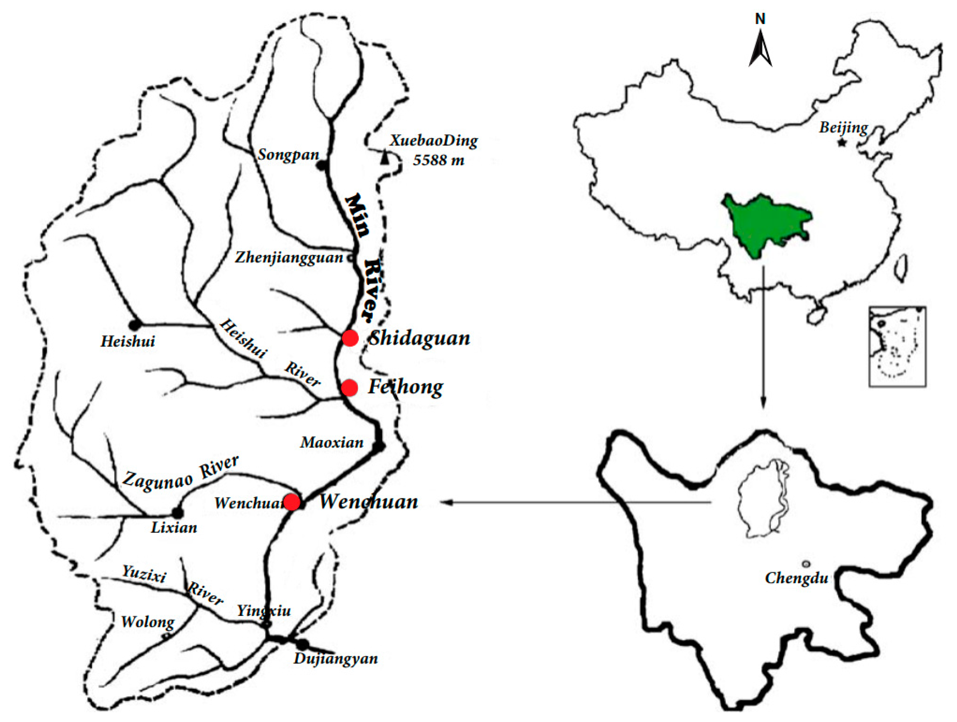
2.1. Study Area
2.2. Data Collection
2.3. Vegetation Structure Metrics
2.4. Spatial Variables
2.5. Data Analysis
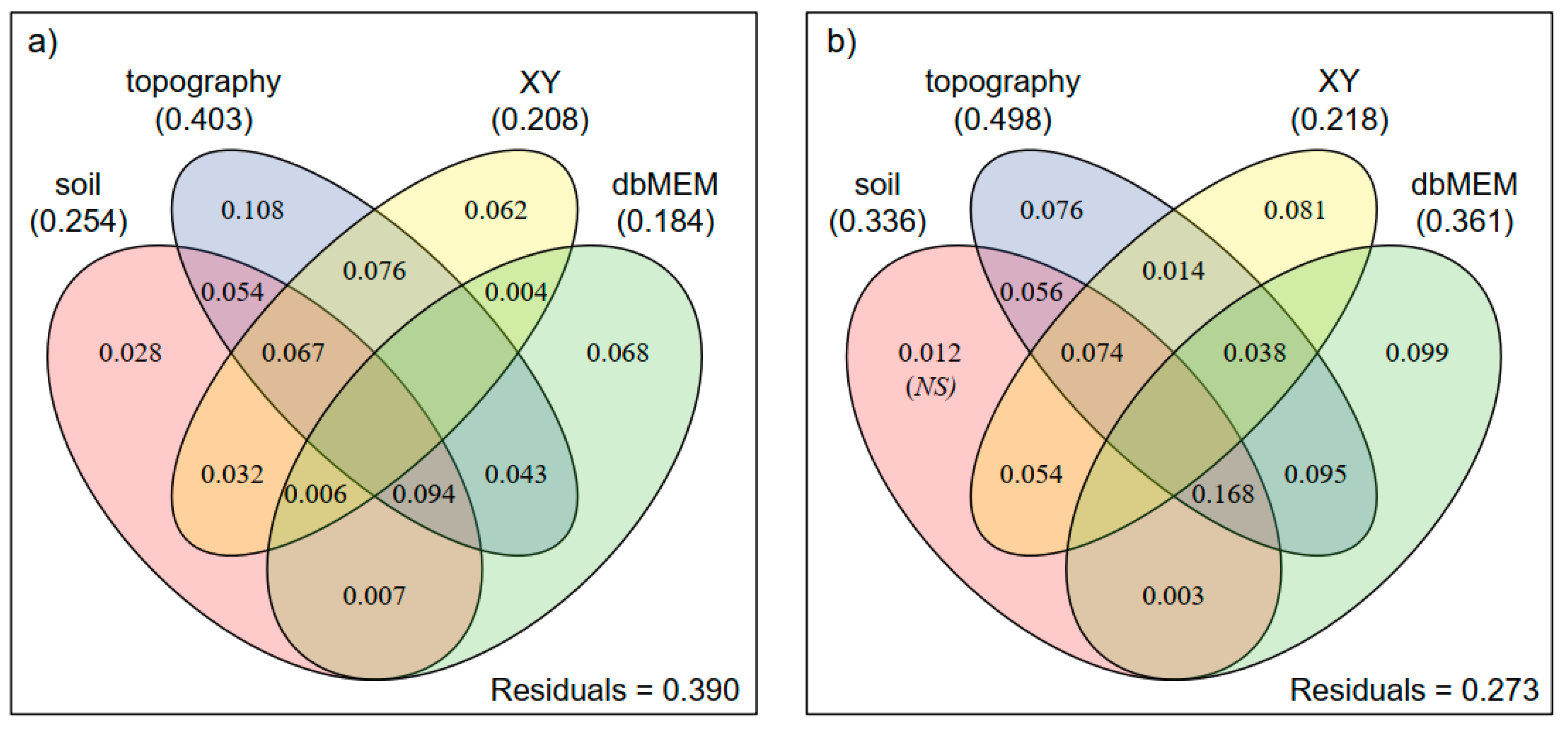
3. Results
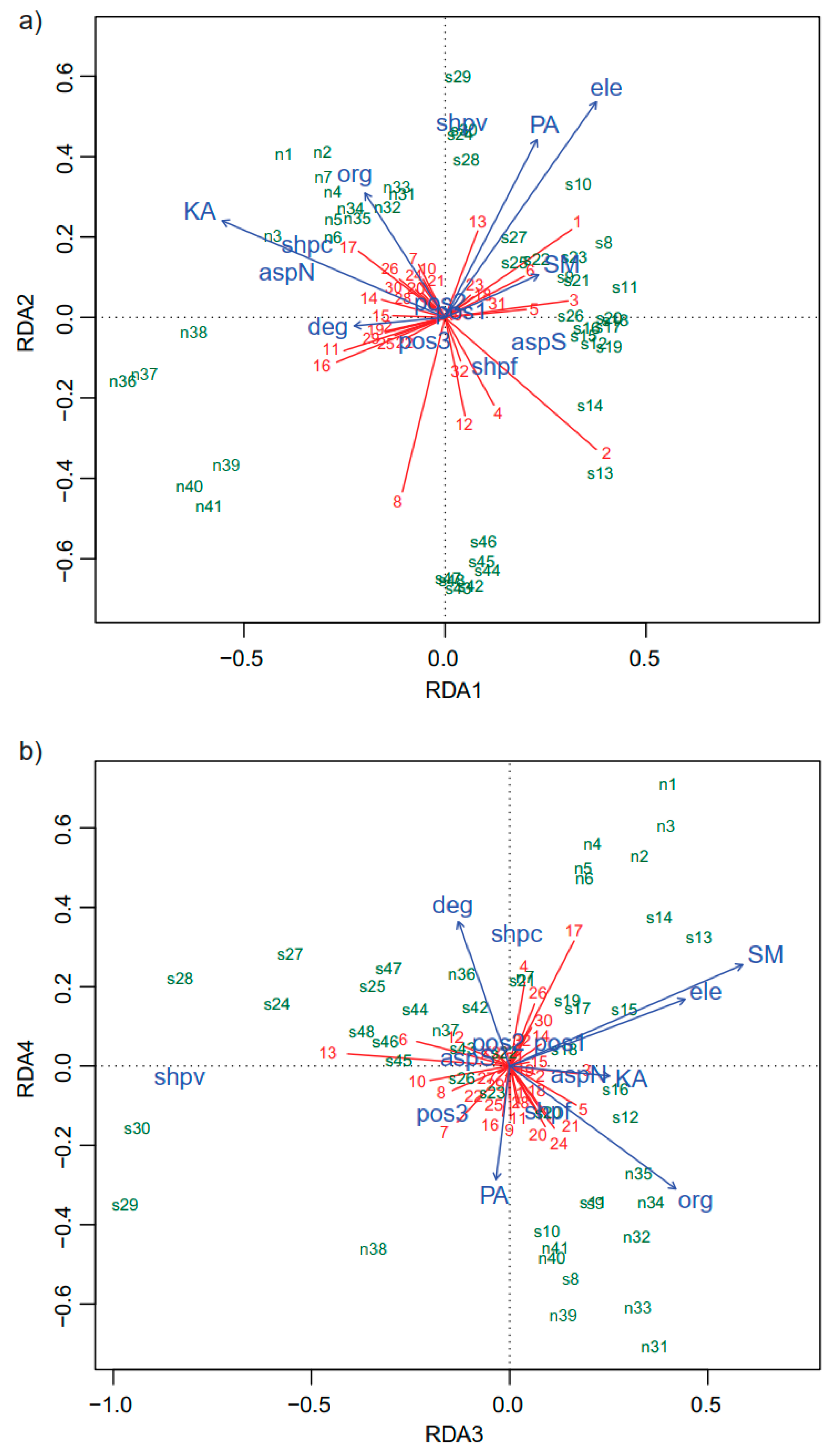
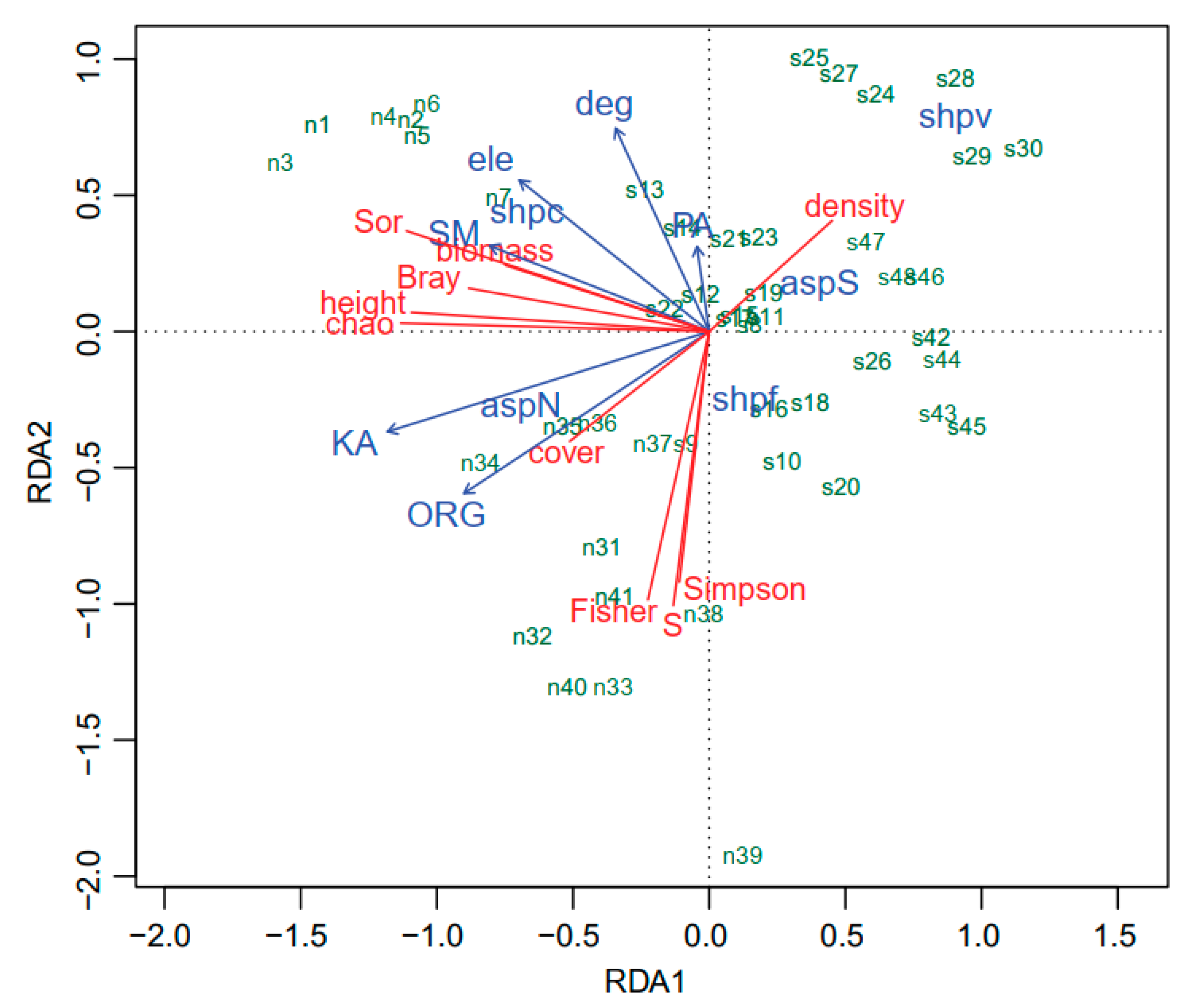
3.1. Community Composition
3.2. Vegetation Structure
4. Discussion
5. Conclusions
Author Contributions
Funding
Acknowledgments
Conflicts of Interest
Data Availability Statement
References
- Bellard, C.; Bertelsmeier, C.; Leadley, P.; Thuiller, W.; Courchamp, F. Impacts of climate change on the future of biodiversity. Ecol. Lett. 2012, 15, 365–377. [Google Scholar] [CrossRef] [Green Version]
- Socolar, J.B.; Gilroy, J.J.; Kunin, W.E.; Edwards, D.P. How Should Beta-Diversity Inform Biodiversity Conservation? Trends Ecol. Evol. 2016, 31, 67–80. [Google Scholar] [CrossRef] [PubMed] [Green Version]
- Chase, J.M.; Leibold, M.A. Ecological Niches: Linking Classical and Contemporary Approaches; University of Chicago Press: Chicago, IL, USA, 2003. [Google Scholar]
- Silvertown, J. Plant coexistence and the niche. Trends Ecol. Evol. 2004, 19, 605–611. [Google Scholar] [CrossRef]
- Hubbell, S. The Unified Neutral Theory of Biodiversity and Biogeography; Princeton University Press: Princeton, NJ, USA, 2001. [Google Scholar]
- Chave, J. Neutral theory and community ecology. Ecol. Lett. 2004, 7, 241–253. [Google Scholar] [CrossRef]
- Cottenie, K. Integrating environmental and spatial processes in ecological community dynamics. Ecol. Lett. 2005, 8, 1175–1182. [Google Scholar] [CrossRef]
- Tilman, D. Niche tradeoffs, neutrality, and community structure: A stochastic theory of resource competition, invasion, and community assembly. Proc. Natl. Acad. Sci. USA 2004, 101, 10854–10861. [Google Scholar] [CrossRef] [Green Version]
- Gravel, D.; Canham, C.D.; Beaudet, M.; Messier, C. Reconciling niche and neutrality: The continuum hypothesis. Ecol. Lett. 2006, 9, 399–409. [Google Scholar] [CrossRef] [Green Version]
- Leibold, M.A.; McPeek, M.A. Coexistence of the niche and neutral perspectives in community ecology. Ecology 2006, 87, 1399–1410. [Google Scholar] [CrossRef]
- Haegeman, B.; Loreau, M. A mathematical synthesis of niche and neutral theories in community ecology. J. Theor. Biol. 2011, 269, 150–165. [Google Scholar] [CrossRef] [Green Version]
- Condit, R.; Pitman, N.; Leigh, E.G.; Chave, J.; Terborgh, J.; Foster, R.B.; Nunez, P.; Aguilar, S.; Valencia, R.; Villa, G.; et al. Beta-Diversity in Tropical Forest Trees. Science 2002, 295, 666–669. [Google Scholar] [CrossRef] [Green Version]
- Tuomisto, H.; Ruokolainen, K.; Yli-Halla, M. Dispersal, environment, and floristic variation of western Amazonian forests. Science 2003, 299, 241–244. [Google Scholar] [CrossRef] [PubMed]
- Myers, J.A.; Chase, J.M.; Jimenez, I.; Jorgensen, P.M.; Araujo-Murakami, A.; Paniagua-Zambrana, N.; Seidel, R. Beta-diversity in temperate and tropical forests reflects dissimilar mechanisms of community assembly. Ecol. Lett. 2013, 16, 151–157. [Google Scholar] [CrossRef] [PubMed]
- Harrison, S.; Davies, K.F.; Safford, H.D.; Viers, J.H. Beta diversity and the scale-dependence of the productivity-diversity relationship: A test in the Californian serpentine flora. J. Ecol. 2006, 94, 110–117. [Google Scholar] [CrossRef]
- Murphy, S.J.; Salpeter, K.; Comita, L.S. Higher beta-diversity observed for herbs over woody plants is driven by stronger habitat filtering in a tropical understory. Ecology 2016, 97, 2074–2084. [Google Scholar] [CrossRef] [PubMed]
- Chase, J.M. Spatial scale resolves the niche versus neutral theory debate. J. Veg. Sci. 2014, 25, 319–322. [Google Scholar] [CrossRef]
- Viana, D.S.; Chase, J.M. Spatial scale modulates the inference of metacommunity assembly processes. Ecology 2019, 100. [Google Scholar] [CrossRef]
- Wiens, J.A. Spatial Scaling in Ecology. Funct. Ecol. 1989, 3, 385. [Google Scholar] [CrossRef]
- Levin, S.A. The problem of pattern and scale in ecology. Ecology 1992, 73, 1943–1967. [Google Scholar] [CrossRef]
- Aiello-Lammens, M.E.; Slingsby, J.A.; Merow, C.; Mollmann, H.K.; Euston-Brown, D.; Jones, C.S.; Silander, J.A., Jr. Processes of community assembly in an environmentally heterogeneous, high biodiversity region. Ecography 2017, 40, 561–576. [Google Scholar] [CrossRef]
- Legendre, P.; Mi, X.; Ren, H.; Ma, K.; Yu, M.; Sun, I.; He, F. Partitioning beta diversity in a subtropical broad-leaved forest of China. Ecology 2009, 90, 663–674. [Google Scholar] [CrossRef] [Green Version]
- Shipley, B.; Paine, C.E.T.; Baraloto, C. Quantifying the importance of local niche-based and stochastic processes to tropical tree community assembly. Ecology 2012, 93, 760–769. [Google Scholar] [CrossRef] [Green Version]
- Van Breugel, M.; Craven, D.; Lai, H.R.; Baillon, M.; Turner, B.L.; Hall, J.S. Soil nutrients and dispersal limitation shape compositional variation in secondary tropical forests across multiple scales. J. Ecol. 2019, 107, 566–581. [Google Scholar] [CrossRef]
- Borcard, D.; Legendre, P. All-scale spatial analysis of ecological data by means of principal coordinates of neighbour matrices. Ecol. Model. 2002, 153, 51–68. [Google Scholar] [CrossRef]
- Borcard, D.; Legendre, P.; Avois-Jacquet, C.; Tuomisto, H. Dissecting the spatial structure of ecological data at multiple scales. Ecology 2004, 85, 1826–1832. [Google Scholar] [CrossRef] [Green Version]
- Dray, S.; Legendre, P.; Peres-Neto, P.R. Spatial modelling: A comprehensive framework for principal coordinate analysis of neighbour matrices (PCNM). Ecol. Model. 2006, 196, 483–493. [Google Scholar] [CrossRef]
- Laliberte, E.; Paquette, A.; Legendre, P.; Bouchard, A. Assessing the scale-specific importance of niches and other spatial processes on beta diversity: A case study from a temperate forest. Oecologia 2009, 159, 377–388. [Google Scholar] [CrossRef] [PubMed]
- Menezes, L.D.; Muller, S.C.; Overbeck, G.E. Scale-specific processes shape plant community patterns in subtropical coastal grasslands. Austral Ecol. 2016, 41, 65–73. [Google Scholar] [CrossRef]
- Page, N.V.; Shanker, K. Environment and dispersal influence changes in species composition at different scales in woody plants of the Western Ghats, India. J. Veg. Sci. 2018, 29, 74–83. [Google Scholar] [CrossRef] [Green Version]
- Yuan, Z.Q.; Gazol, A.; Wang, X.; Lin, F.; Ye, J.; Bai, X.; Li, B.; Hao, Z. Scale specific determinants of tree diversity in an old growth temperate forest in China. Basic Appl. Ecol. 2011, 12, 488–495. [Google Scholar] [CrossRef]
- Dray, S.; Pelissier, R.; Couteron, P.; Fortin, M.; Legendre, P.; Peres-Neto, P.R.; Bellier, E.; Bivand, R.; Blanchet, F.G.; de Caceres, M.; et al. Community ecology in the age of multivariate multiscale spatial analysis. Ecol. Monogr. 2012, 82, 257–275. [Google Scholar] [CrossRef]
- Guèze, M.; Paneque-Galvez, J.; Luz, A.C.; Pino, J.; Orta-Martinez, M.; Reyes-Garcia, V.; Macia, M.J. Determinants of tree species turnover in a southern Amazonian rain forest. J. Veg. Sci. 2013, 24, 284–295. [Google Scholar] [CrossRef]
- Pashirzad, M.; Ejtehadi, H.; Vaezi, J.; Shefferson, R.P. Multiple processes at different spatial scales determine beta diversity patterns in a mountainous semi-arid rangeland of Khorassan-Kopet Dagh floristic province, NE Iran. Plant Ecol. 2019, 220, 829–844. [Google Scholar] [CrossRef]
- Smith, R.J.; Stark, L.R. Habitat vs. dispersal constraint’s on bryophyte diversity in the Mojave Desert, USA. J. Arid Environ. 2014, 102, 76–81. [Google Scholar] [CrossRef]
- Safriel, U.; Adeel, Z.; Niemeijer, D.; Puigdefabregas, J.; White, R.; Lal, R.; Winslow, M.; Ziedler, J.; Prince, S.; Archer, E.; et al. Findings of the Condition and Trends Working Group. In Ecosystems and Human Well-Being: Current State and Trends; Island Press: Washington, DC, USA, 2005; pp. 623–662. [Google Scholar]
- Feng, S.; Fu, Q. Expansion of global drylands under a warming climate. Atmos. Chem. Phys. 2013, 13, 10081–10094. [Google Scholar] [CrossRef] [Green Version]
- Huang, J.; Yu, H.; Guan, X.; Wang, G.; Guo, R. Accelerated dryland expansion under climate change. Nat. Clim. Chang. 2016, 6, 166. [Google Scholar] [CrossRef]
- Davies, K.W.; Bates, J.D.; Miller, R.F. Environmental and vegetation relationships of the Artemisia tridentata spp. wyomingensis alliance. J. Arid Environ. 2007, 70, 478–494. [Google Scholar] [CrossRef]
- Maestre, F.T.; Cortina, J. Spatial patterns of surface soil properties and vegetation in a Mediterranean semi-arid steppe. Plant Soil 2002, 241, 279–291. [Google Scholar] [CrossRef]
- Poulos, H.M.; Camp, A.E. Topographic influences on vegetation mosaics and tree diversity in the Chihuahuan Desert Borderlands. Ecology 2010, 91, 1140–1151. [Google Scholar] [CrossRef]
- Solon, J.; Degórski, M.; Roo-Zielińska, E. Vegetation response to a topographical-soil gradient. CATENA 2007, 71, 309–320. [Google Scholar] [CrossRef]
- Zhang, R. The Dry Valley of the Hengduan Mountains Regions; Science Press: Beijing, China, 1992. [Google Scholar]
- Guan, W.; Ye, M.S.; Ma, K.M.; Liu, G.H.; Wang, X.L. Vegetation Classification and the Main Types of Vegetation of the Dry Valley of Minjiang River. J. Mt. Res. 2004, 22, 679–686. [Google Scholar]
- Xu, X.-L.; Ma, K.-M.; Fu, B.-J.; Song, C.-J.; Liu, W. Relationships between vegetation and soil and topography in a dry warm river valley, SW China. CATENA 2008, 75, 138–145. [Google Scholar] [CrossRef]
- Ma, K.-M.; Fu, B.; Liu, S.; Guan, W.; Liu, G.; Lu, Y.; Anand, M. Multiple-scale soil moisture distribution and its implications for ecosystem restoration in an arid river valley, China. Land Degrad. Dev. 2004, 15, 75–85. [Google Scholar] [CrossRef]
- Lu, T.; Ma, K.M.; Zhang, W.H.; Fu, B.J. Differential responses of shrubs and herbs present at the Upper Minjiang River basin (Tibetan Plateau) to several soil variables. J. Arid Environ. 2006, 67, 373–390. [Google Scholar] [CrossRef]
- Maestre, F.T.; Eldridge, D.J.; Soliveres, S.; Kefi, S.; Delgado-Baquerizo, M.; Bowker, M.A.; Garcia-Palacios, P.; Gaitan, J.; Gallardo, A.; Lazaro, R.; et al. Structure and Functioning of Dryland Ecosystems in a Changing World. Ann. Rev. Ecol. Evol. System. 2016, 47, 215–237. [Google Scholar] [CrossRef] [Green Version]
- Pang, X.Y.; Bao, W.K.; Ning, W.U. Reasons of dry valley climate characteristic and its formation reason in upstream of Minjiang River. Resour. Environ. Yangtze Basin 2008, 17, 46–53. [Google Scholar]
- Vegetation, E.B.o.S. Sichuan Vegetation; People’s Publishing House of Sichuan: Chengdu, China, 1980. [Google Scholar]
- Maurer, B.A.; McGill, B.J. Biological Diversity: Frontiers in Measurement and Assessment; Magurran, A.E., McGill, B.J., Eds.; Oxford University Press: Oxford, UK, 2011; pp. 55–65. [Google Scholar]
- Fisher, R.A.; Corbet, A.S.; Williams, C.B. The relation between the number of species and the number of individuals in a random sample of an animal population. J. Anim. Ecol. 1943, 42–58. [Google Scholar] [CrossRef]
- Koleff, P.; Gaston, K.J.; Lennon, J.J. Measuring beta diversity for presence–absence data. J. Anim. Ecol. 2003, 72, 367–382. [Google Scholar] [CrossRef] [Green Version]
- Sørensen, T.A. A method of establishing groups of equal amplitude in plant sociology based on similarity of species content and its application to analyses of the vegetation on Danish commons. Kongelige Danske Videnskabernes Selskabs Biol. Skrifter 1948, 5, 1–34. [Google Scholar]
- Bray, J.R.; Curtis, J.T. An ordination of the upland forest communities of southern Wisconsin. Ecol. Monogr. 1957, 27, 325–349. [Google Scholar] [CrossRef]
- Chao, A.; Chazdon, R.L.; Colwell, R.K.; Shen, T.-J. A new statistical approach for assessing similarity of species composition with incidence and abundance data. Ecol. Lett. 2005, 8, 148–159. [Google Scholar] [CrossRef]
- Oksanen, J.; Blanchet, F.G.; Kindt, R.; Legendre, P.; Minchin, P.R.; O’hara, R.B.; Simpson, G.L.; Solymos, P.; Stevens, M.H.H.; Wagner, H. Vegan: Community Ecology Package. R Package Ver. 2.5-2 2018, 2. [Google Scholar]
- Declerck, S.A.J.; Coronel, J.S.; Legendre, P.; Brendonck, L. Scale dependency of processes structuring metacommunities of cladocerans in temporary pools of High-Andes wetlands. Ecography 2011, 34, 296–305. [Google Scholar] [CrossRef] [Green Version]
- adespatial: Multivariate Multiscale Spatial Analysis. R Package Version 0.3–8. Available online: https://CRAN.R-project.org/package=adespatial (accessed on 3 April 2018).
- Ter Braak, C.J.F. Canonical Correspondence Analysis: A New Eigenvector Technique for Multivariate Direct Gradient Analysis. Ecology 1986, 67, 1167–1179. [Google Scholar] [CrossRef] [Green Version]
- Blanchet, F.G.; Legendre, P.; Borcard, D. Forward selection of explanatory variables. Ecology 2008, 89, 2623–2632. [Google Scholar] [CrossRef] [PubMed]
- Borcard, D.; Gillet, F.; Legendre, P. Numerical Ecology with R; Springer: Berlin/Heidelberg, Germany, 2018. [Google Scholar]
- Borcard, D.; Legendre, P.; Drapeau, P. Partialling out the Spatial Component of Ecological Variation. Ecology 1992, 73, 1045–1055. [Google Scholar] [CrossRef] [Green Version]
- Peres-Neto, P.R.; Legendre, P.; Dray, S.; Borcard, D. Variation partitioning of species data matrices: Estimation and comparision of fractions. Ecology 2006, 87, 2614–2625. [Google Scholar] [CrossRef]
- Legendre, P.; Gallagher, E.D. Ecologically meaningful transformations for ordination of species data. Oecologia 2001, 129, 271–280. [Google Scholar] [CrossRef] [PubMed]
- RFfSC R Core Team. R: A Language and Environment for Statistical Computing; R foundation for statistical computing: Vienna, Austria, 2013. [Google Scholar]
- Cantón, Y.; Del Barrio, G.; Solé-Benet, A.; Lázaro, R. Topographic controls on the spatial distribution of ground cover in the Tabernas badlands of SE Spain. CATENA 2004, 55, 341–365. [Google Scholar] [CrossRef]
- Bennie, J.; Hill, M.O.; Baxter, R.; Huntley, B. Influence of slope and aspect on long-term vegetation change in British chalk grasslands. J. Ecol. 2006, 94, 355–368. [Google Scholar] [CrossRef]
- Jafari, M.; Chahouki, M.A.Z.; Tavili, A.; Azarnivand, H.; Amiri, G.Z. Effective environmental factors in the distribution of vegetation types in Poshtkouh rangelands of Yazd Province (Iran). J. Arid Environ. 2004, 56, 627–641. [Google Scholar] [CrossRef]
- Bennie, J.; Huntley, B.; Wiltshire, A.; Hill, M.O.; Baxter, R. Slope, aspect and climate: Spatially explicit and implicit models of topographic microclimate in chalk grassland. Ecol. Model. 2008, 216, 47–59. [Google Scholar] [CrossRef]
- McCune, B.; Keon, D. Equations for potential annual direct incident radiation and heat load. J. Veg. Sci. 2002, 13, 603–606. [Google Scholar] [CrossRef]
- Pueyo, Y.; Alados, C.L.; Maestro, M.; Komac, B. Gypsophile vegetation patterns under a range of soil properties induced by topographical position. Plant Ecol. 2007, 189, 301–311. [Google Scholar] [CrossRef]
- Moeslund, J.E.; Arge, L.; Bocher, P.K.; Dalgaard, T.; Ejrnaes, R.; Odgaard, M.V.; Svenning, J. Topographically controlled soil moisture drives plant diversity patterns within grasslands. Biodivers. Conserv. 2013, 22, 2151–2166. [Google Scholar] [CrossRef]
- Desta, F.; Colbert, J.J.; Rentch, J.S.; Gottschalk, K.W. Aspect induced differences in vegetation, soil, and microclimatic characteristics of an Appalachian watershed. Castanea 2004, 69, 92–108. [Google Scholar] [CrossRef]
- Li, Y.J.; Bao, W.K.; Wu, N. Spatial patterns of the soil seed bank and extant vegetation across the dry Minjiang River valley in southwest China. J. Arid Environ. 2011, 75, 1083–1089. [Google Scholar] [CrossRef]
- Cantlon, J.E. Vegetation and Microclimates on North and South Slopes of Cushetunk Mountain, New Jersey. Ecol. Monogr. 1953, 23, 241–270. [Google Scholar] [CrossRef]
- Holland, P.G.; Steyn, D.G. Vegetational Responses to Latitudinal Variations in Slope Angle and Aspect. J. Biogeogr. 1975, 2, 179–183. [Google Scholar] [CrossRef]
- Badano, E.I.; Cavieres, L.A.; Molina-Montenegro, M.A.; Quiroz, C. Slope aspect influences plant association patterns in the Mediterranean matorral of central Chile. J. Arid Environ. 2005, 62, 93–108. [Google Scholar] [CrossRef]
- Zapata-Rios, X.; Brooks, P.D.; Troch, P.A.; McIntosh, J.; Guo, Q. Influence of terrain aspect on water partitioning, vegetation structure and vegetation greening in high-elevation catchments in northern New Mexico. Ecohydrology 2016, 9, 782–795. [Google Scholar] [CrossRef]
- Moore, I.D.; Grayson, R.B.; Ladson, A.R. Digital terrain modelling: A review of hydrological, geomorphological, and biological applications. Hydrol. Process. 1991, 5, 3–30. [Google Scholar] [CrossRef]
- Zaslavsky, D.; Sinai, G. Surface Hydrology: I—Explanation of Phenomena. J. Hydraul. Div. 1981, 107, 16. [Google Scholar]
- Liu, G.; Keming, M.; Bojie, F.; Wenbin, G.; Yongxiang, K.; Jianyun, Z.; Shiliang, L. Aboveground biomass of main shrubs in dry valley of Minjiang River. Acta Ecol. Sin. 2003, 23, 1757–1764. [Google Scholar] [CrossRef]
- Song, C.J.; Ma, K.M.; Fu, B.J.; Qu, L.Y.; Xu, X.L.; Liu, Y.; Zhong, J.F. Distribution patterns of shrubby N-fixers and non-N fixers in an arid valley in Southwest China: Implications for ecological restoration. Ecol. Res. 2010, 25, 553–564. [Google Scholar] [CrossRef]
- Gong, X.; Brueck, H.; Giese, K.M.; Zhang, L.; Sattelmacher, B.; Lin, S. Slope aspect has effects on productivity and species composition of hilly grassland in the Xilin River Basin, Inner Mongolia, China. J. Arid Environ. 2008, 72, 483–493. [Google Scholar] [CrossRef]
- Måren, I.E.; Karki, S.; Prajapati, C.; Yadav, R.K.; Shrestha, B.B. Facing north or south: Does slope aspect impact forest stand characteristics and soil properties in a semiarid trans-Himalayan valley? J. Arid Environ. 2015, 121, 112–123. [Google Scholar] [CrossRef] [Green Version]
- Adler, P.B.; Seabloom, E.W.; Borer, E.T.; Hillebrand, H.; Hautier, Y.; Hector, A.; Harpole, W.S.; O’Halloran, L.R.; Grace, J.B.; Anderson, T.M.; et al. Productivity Is a Poor Predictor of Plant Species Richness. Science 2011, 333, 1750–1753. [Google Scholar] [CrossRef] [Green Version]
- Chase, J.M.; Leibold, M.A. Spatial scale dictates the productivity–biodiversity relationship. Nature 2002, 416, 427–430. [Google Scholar] [CrossRef]
- Grime, J.P. Competitive Exclusion in Herbaceous Vegetation. Nature 1973, 242, 344–347. [Google Scholar] [CrossRef]
- Chase, J.M. Stochastic Community Assembly Causes Higher Biodiversity in More Productive Environments. Science 2010, 328, 1388–1391. [Google Scholar] [CrossRef] [Green Version]
- Fllner, S.; Shmida, A. Why are adaptations for long-range seed dispersal rare in desert plants? Oecologia 1981, 51, 133–144. [Google Scholar] [CrossRef]
- Li, Y.; Bao, W.; Wu, F. Soil seed bank and natural regeneration potential of shrubland in dry valleys of Minjiang river. Acta Ecol. Sin. 2010, 30, 399–407. [Google Scholar]
- He, M.Z.; Zheng, J.G.; Li, X.R.; Qian, Y.L. Environmental factors affecting vegetation composition in the Alxa Plateau, China. J. Arid Environ. 2007, 69, 473–489. [Google Scholar] [CrossRef]
- Chang, L.W.; Zeleny, D.; Li, C.F.; Chiu, S.T.; Hsieh, C.F. Better environmental data may reverse conclusions about niche- and dispersal-based processes in community assembly. Ecology 2013, 94, 2145–2151. [Google Scholar] [CrossRef]
- Jones, M.M.; Tuomisto, H.; Borcard, D.; Legendre, P.; Clark, D.B.; Olivas, P.C. Explaining variation in tropical plant community composition: Influence of environmental and spatial data quality. Oecologia 2008, 155, 593–604. [Google Scholar] [CrossRef]


| Site | Latitude | Longitude | Elevation (m) | Temperature (°C) | N 1 |
|---|---|---|---|---|---|
| Shidaguan | 31.8980° | 103.6962° | 2027 | 8.7 | 23 |
| Feihong | 31.7993° | 103.7394° | 1853 | 11.9 | 12 |
| Wenchuan | 31.4698° | 103.5756° | 1433 | 13.5 | 13 |
| Community Composition | Vegetation Structure | |||||||
|---|---|---|---|---|---|---|---|---|
| R2adj | Df | F | p | R2adj | Df | F | p | |
| Total | 0.610 | 16 | 5.596 | 0.001 | 0.727 | 15 | 9.357 | 0.001 |
| Based on Four Subsets | ||||||||
| soil | 0.254 | 4 | 5.001 | 0.001 | 0.336 | 4 | 6.941 | 0.001 |
| soil/(topo+XY+dbMEM) | 0.028 | 4 | 1.625 | 0.004 | 0.012 NS | 4 | 1.411 | 0.096 |
| topo | 0.403 | 7 | 5.529 | 0.001 | 0.498 | 5 | 10.320 | 0.001 |
| topo/(soil+XY+dbMEM) | 0.108 | 7 | 2.502 | 0.001 | 0.076 | 5 | 3.053 | 0.001 |
| XY | 0.208 | 2 | 7.185 | 0.001 | 0.218 | 2 | 7.535 | 0.001 |
| XY/(soil+topo+dbMEM) | 0.062 | 2 | 3.611 | 0.001 | 0.081 | 2 | 6.047 | 0.001 |
| dbMEM | 0.184 | 3 | 6.410 | 0.001 | 0.361 | 4 | 7.639 | 0.001 |
| dbMEM/(soil+topo+XY) | 0.068 | 3 | 2.990 | 0.001 | 0.099 | 4 | 4.252 | 0.001 |
| Based on Two Subsets | ||||||||
| env | 0.476 | 11 | 4.880 | 0.001 | 0.559 | 9 | 7.610 | 0.001 |
| env/spa | 0.190 | 11 | 2.857 | 0.001 | 0.144 | 9 | 3.411 | 0.001 |
| spa | 0.420 | 5 | 7.817 | 0.001 | 0.583 | 6 | 11.951 | 0.001 |
| spa/env | 0.134 | 5 | 3.477 | 0.001 | 0.169 | 6 | 4.918 | 0.001 |
| Community Composition | Vegetation Structure | ||||||||
|---|---|---|---|---|---|---|---|---|---|
| Df | Variance | F | Pr (>F) | Df | Variance | F | Pr (>F) | ||
| Regional scale | ele | 1 | 0.041 | 47.956 | 0.001 | 1 | 0.185 | 39.876 | 0.001 |
| shp | 2 | 0.013 | 8.093 | 0.001 | 2 | 0.068 | 7.378 | 0.001 | |
| SM | 1 | 0.009 | 11.421 | 0.001 | 1 | 0.054 | 11.558 | 0.001 | |
| ORG | 1 | 0.013 | 14.784 | 0.001 | 1 | 0.071 | 15.195 | 0.001 | |
| KA | 1 | 0.005 | 5.993 | 0.002 | 1 | 0.026 | 5.705 | 0.006 | |
| Residual | 41 | 0.035 | 41 | 0.19 | |||||
| Df | Variance | F | Pr (>F) | Df | Variance | F | Pr (>F) | ||
| Local scale | ele | — | — | — | — | 1 | 0.021 | 3.81 | 0.029 |
| asp | 1 | 0.044 | 20.781 | 0.001 | 1 | 0.252 | 44.826 | 0.001 | |
| shp | 2 | 0.043 | 10.374 | 0.001 | 2 | 0.254 | 22.568 | 0.001 | |
| deg | 1 | 0.011 | 5.341 | 0.002 | 1 | 0.055 | 9.772 | 0.001 | |
| pos | 2 | 0.01 | 2.368 | 0.023 | — | — | — | — | |
| Residual | 41 | 0.086 | 42 | 0.236 | |||||
| Community Composition | Vegetation Structure | ||||||||
|---|---|---|---|---|---|---|---|---|---|
| RDA1 | RDA2 | RDA3 | RDA4 | RDA5 | RDA1 | RDA2 | RDA3 | RDA4 | |
| Eigenvalue | 0.121 | 0.096 | 0.069 | 0.056 | 0.043 | 3.053 | 1.844 | 0.879 | 0.454 |
| Variation explained | 0.129 | 0.102 | 0.074 | 0.060 | 0.046 | 0.265 | 0.160 | 0.076 | 0.039 |
| Cumulative variation explained | 0.129 | 0.232 | 0.305 | 0.366 | 0.412 | 0.265 | 0.425 | 0.502 | 0.541 |
| Intra-set correlation coefficient | |||||||||
| Organic matter (ORG) | −0.246 | 0.383 ** | 0.505 *** | −0.373 ** | −0.438 ** | −0.563 *** | −0.372 ** | −0.343 * | 0.619 *** |
| Available phosphorus (PA) | 0.283 | 0.547 *** | −0.041 | −0.345 * | 0.229 | −0.028 | 0.195 | −0.382 ** | 0.249 |
| Available potassium (KA) | −0.686 *** | 0.298 * | 0.304 * | −0.030 | 0.171 | −0.739 *** | −0.230 | −0.407 ** | −0.155 |
| Soil moisture (SM) | 0.287 * | 0.131 | 0.708 *** | 0.308 * | 0.246 | −0.504 *** | 0.197 | 0.522 *** | 0.138 |
| Elevation (ele) | 0.465 *** | 0.663 *** | 0.533 *** | 0.203 | 0.090 | −0.436 ** | 0.348 * | 0.216 | 0.383 ** |
| Degree (deg) | −0.280 | −0.026 | −0.156 | 0.438 ** | −0.566 *** | −0.215 | 0.466 *** | −0.144 | 0.242 |
| Aspect (asp) | 0.865 *** | 0.239 | 0.388 ** | 0.059 | 0.140 | 0.790 *** | 0.323 * | 0.380 ** | 0.114 |
| Shape (shp) | 0.567 *** | 0.551 *** | 0.721 *** | 0.544 *** | 0.166 | 0.651 *** | 0.559 *** | 0.735 *** | 0.404 * |
| Position (pos) | 0.106 | 0.109 | 0.336 | 0.207 | 0.281 | — | — | — | — |
| Biomass | Cover | Height | Density | S | Fisher | Simpson | Sorenson | Bray-Curtis | Chao | |
|---|---|---|---|---|---|---|---|---|---|---|
| Biomass | 0.009 | 0.000 | 0.597 | 0.245 | 0.644 | 0.191 | 0.000 | 0.317 | 0.028 | |
| Cover | 0.371 ** | 0.023 | 0.250 | 0.014 | 0.067 | 0.195 | 0.500 | 0.847 | 0.176 | |
| Height | 0.736 *** | 0.327 * | 0.239 | 0.697 | 0.698 | 0.856 | 0.000 | 0.001 | 0.000 | |
| Density | 0.078 | 0.169 | −0.173 | 0.301 | 0.000 | 0.021 | 0.304 | 0.000 | 0.000 | |
| S | −0.171 | 0.354 * | 0.058 | −0.152 | 0.000 | 0.000 | 0.334 | 0.993 | 0.611 | |
| Fisher | −0.068 | 0.267 | 0.058 | −0.515 *** | 0.664 *** | 0.000 | 0.087 | 0.519 | 0.499 | |
| Simpson | −0.192 | 0.190 | 0.027 | -0.332 * | 0.774 *** | 0.772 *** | 0.196 | 0.884 | 0.539 | |
| Sorenson | 0.489 *** | 0.100 | 0.730 *** | −0.152 | −0.142 | −0.250 | −0.190 | 0.000 | 0.000 | |
| Bray-Curtis | 0.147 | −0.029 | 0.463 *** | −0.583 *** | −0.001 | 0.095 | 0.022 | 0.707 *** | 0.000 | |
| Chao | 0.317 | 0.199 | 0.624 *** | −0.486 *** | 0.075 | 0.100 | 0.091 | 0.835 *** | 0.881 *** |
Publisher’s Note: MDPI stays neutral with regard to jurisdictional claims in published maps and institutional affiliations. |
© 2020 by the authors. Licensee MDPI, Basel, Switzerland. This article is an open access article distributed under the terms and conditions of the Creative Commons Attribution (CC BY) license (http://creativecommons.org/licenses/by/4.0/).
Share and Cite
Yang, J.; El-Kassaby, Y.A.; Guan, W. Multiple Ecological Drivers Determining Vegetation Attributes across Scales in a Mountainous Dry Valley, Southwest China. Forests 2020, 11, 1140. https://doi.org/10.3390/f11111140
Yang J, El-Kassaby YA, Guan W. Multiple Ecological Drivers Determining Vegetation Attributes across Scales in a Mountainous Dry Valley, Southwest China. Forests. 2020; 11(11):1140. https://doi.org/10.3390/f11111140
Chicago/Turabian StyleYang, Jie, Yousry A. El-Kassaby, and Wenbin Guan. 2020. "Multiple Ecological Drivers Determining Vegetation Attributes across Scales in a Mountainous Dry Valley, Southwest China" Forests 11, no. 11: 1140. https://doi.org/10.3390/f11111140
APA StyleYang, J., El-Kassaby, Y. A., & Guan, W. (2020). Multiple Ecological Drivers Determining Vegetation Attributes across Scales in a Mountainous Dry Valley, Southwest China. Forests, 11(11), 1140. https://doi.org/10.3390/f11111140