Comparison of Soil Greenhouse Gas Fluxes during the Spring Freeze–Thaw Period and the Growing Season in a Temperate Broadleaved Korean Pine Forest, Changbai Mountains, China

Abstract

Soils in mid-high latitudes are under the great impact of freeze–thaw cycling. However, insufficient research on soil CO₂, CH₄, and N₂O fluxes during the spring freeze–thaw (SFT) period has led to great uncertainties in estimating soil greenhouse gas (GHG) fluxes. The present study was conducted in a temperate broad-leaved Korean pine mixed forest in Northeastern China, where soils experience an apparent freeze–thaw effect in spring. The temporal variations and impact factors of soil GHG fluxes were measured during the SFT period and growing season (GS) using the static-chamber method. The results show that the soil acted as a source of atmospheric CO₂ and N₂O and a sink of atmospheric CH₄ during the whole observation period. Soil CO₂ emission and CH₄ uptake were lower during the SFT period than those during the GS, whereas N₂O emissions were more than six times higher during the SFT period than that during the GS. The responses of soil GHG fluxes to soil temperature (T_s) and soil moisture during the SFT and GS periods differed. During the SFT period, soil CO₂ and CH₄ fluxes were mainly affected by the volumetric water content (VWC) and T_s, respectively, whereas soil N₂O flux was influenced jointly by T_s and VWC. The dominant controlling factor for CO₂ was T_s during the GS, whereas CH₄ and N₂O were mainly regulated by VWC. Soil CO₂ and N₂O fluxes accounted for 97.3% and 3.1% of the total 100-year global warming potential (GWP₁₀₀) respectively, with CH₄ flux offsetting 0.4% of the total GWP₁₀₀. The results highlight the importance of environmental variations to soil N₂O pulse during the SFT period and the difference of soil GHG fluxes between the SFT and GS periods, which contribute to predicting the forest soil GHG fluxes and their global warming potential under global climate change.

1. Introduction

Carbon dioxide (CO₂), methane (CH₄), and nitrous oxide (N₂O) are recognised as the most important greenhouse gases (GHGs), as their contributions to the 100-year global warming potential (GWP₁₀₀), indicating the warming ability of each GHG over 100 years [1,2,3,4], have reached 60%, 15%, and 5%, respectively [5]. According to the fifth assessment report of the Intergovernmental Panel on Climate Change (IPCC), atmospheric GHG concentrations have reached their highest levels in the past 80 years [2]. Soil–atmosphere GHG exchanges have a considerable impact on global climate change by largely affecting atmospheric GHG concentrations [2,6]. This is because the carbon (C) and nitrogen (N) stocks of soils are vital parts of C and N pools in terrestrial ecosystems [7,8]. In forest ecosystems, soil C stocks are approximately two-thirds of the total C content [9,10], whereas soil N stocks account for >85% of the total N content [11]. Therefore, soils play an irreplaceable role in slowing the rise of atmospheric GHG concentrations, maintaining the global C and N balance, and regulating global climate change.

Soil–atmosphere GHG exchanges are jointly regulated by multiple biophysical and biochemical processes [6] and are synergistically regulated by various environmental factors (e.g., temperature, precipitation, and soil moisture) and biological factors (e.g., labile C and N supply and microbial activity) [6,12,13,14]. The variations in soil temperature (T_s) and soil moisture are considered to be the most important factors influencing seasonal variations in soil GHG fluxes [6,15,16,17,18]. Many studies have found that T_s and soil moisture are the dominant drivers to soil CO₂ and N₂O emissions and soil CH₄ uptake [3,6,13,15]. This is because the optimal T_s and moisture increase soil microbial activities, which promote the decomposition of soil organic matter, soil nitrification, and denitrification as well as the metabolism of methane-oxidising bacteria [19,20,21,22]. However, the increases in T_s may also trigger water stress, leading to the inhibition of soil organic matter mineralisation, nitrification, and denitrification, thereby reducing soil CO₂ and N₂O emissions [23,24], CH₄ uptake [25], and even changing soil from a CH₄ sink to a CH₄ source [6,7,26]. Similarly, the increase in the soil volumetric water content (VWC) can inhibit soil CO₂ and N₂O emissions and soil CH₄ uptake [27,28,29]. Hence, there remain large uncertainties regarding the responses of soil GHG fluxes to environmental changes. In addition, the correlations between soil GHG fluxes and environmental factors are complicated, generally presenting a nonlinear relationship [30] and are strongly affected by the interactive effects of T_s and moisture [31,32,33].

The soil freeze–thaw cycle (FTC) is the phenomenon of repeated soil freezing and thawing caused by seasonal or diurnal temperature changes [26,34,35]. Approximately 57% of the exposed land surfaces in the Northern Hemisphere experience soil FTCs, which greatly impact soil C and N cycles [36]. However, soil CO₂, CH₄, and N₂O fluxes in the non-growing season, especially during the spring freeze–thaw (SFT) period, have rarely been reported [19,37]. Frequent measurements during the SFT period can promote an advanced understanding of the responses of soil processes to a rapidly changing environment. The soil phase transition and its accompanying phenomena during an FTC lead to the changes in T_s, VWC, and other soil physical properties, which have further impacts on the morphological transformation of soil organic and inorganic matter as well as soil chemical properties and microbial activity [38,39]. Thus, FTCs substantially contribute to the change of soil GHG fluxes [26,40]. Global climate models predict that future climate change is likely to alter the frequency and intensity of soil freeze–thaw processes, implying that the influence of freeze–thaw events is becoming increasingly prominent [37,41,42]. Numerous studies have shown that CO₂ and N₂O emissions, as well as CH₄ uptake, have increased during FTCs [26,37,43,44]. The dynamics of soil GHG fluxes during FTCs were considered to be mainly caused by stimulated microbial metabolism and improved soil physical and chemical properties, due to the substrate supply and various physical mechanisms [20,26,39,45,46]. By assessing soil GHG fluxes under FTCs from 23 forest ecosystems, Kim et al. found that soil texture, forest type, soil moisture, and the length of the thawing period contribute to the generation of N₂O [40]. Meanwhile, they also found that freezing temperature, available substrate, O₂ concentration, and the frequency of freeze–thaw events drive the generation of CH₄ and CO₂. Similarly, other studies found that the soil GHG fluxes are influenced by the FTC frequency and the spatial heterogeneity of soil T_s and VWC during an FTC [32,47]. However, the role of FTCs in affecting soil GHG fluxes remains unclear due to the complicated influencing mechanism of the soil freeze–thaw process on soil C and N cycles. Hence, the characterisation of the differences in the dynamic changes of soil GHG fluxes during the SFT period and the growing season (GS), as well as their feedback on global climate changes, would contribute to improving our understanding of the mechanisms of soil GHG emissions, thereby enabling accurate estimations of C and N budgets.

The broad-leaved Korean pine mixed forest in the Changbai Mountains (CBF) is a typical zonal climax forest in the temperate zone of China [48,49,50]. Previous studies have shown that the forest soil in the CBF is a source of CO₂ and N₂O as well as a CH₄ sink. In addition, soil GHG dynamics are mainly affected by environmental factors (e.g., temperature, precipitation, and soil moisture), C and N concentrations, and soil microorganisms [51,52,53,54]. However, previous studies were mainly focussed on CO₂ flux; few studies have assessed other GHGs (e.g., CH₄ and N₂O) [8,55], especially during the SFT period [32,56]. Moreover, the relationships between soil GHG fluxes and their main environmental factors in the CBF during the SFT and GS periods remain poorly understood. Based on the static-chamber method, the present study continuously observed soil CO₂, CH₄, and N₂O fluxes in the CBF during an SFT period and a subsequent GS in 2019. Our objectives are to (1) identify the temporal variation patterns of soil GHG fluxes and their relationships; (2) compare the responses of soil GHG fluxes to T_s and VWC between the SFT and GS periods; and (3) to determine the relative contributions of soil GHG fluxes to the warming potential.

2. Materials and Methods

2.1. Site Description

The study was conducted in a broad-leaved Korean pine mixed forest in the Changbai Mountains (42°24′9′′N, 128°05′45′′E, 738 m a.s.l.) in Jilin Province, Northeastern China. The climate in this region is a temperate continental monsoon climate with long winters and short temperate summers. The snow cover period lasts for nearly five months, from late fall to early mid-spring [57,58]. The mean annual temperature is 3.6 °C (8.7 to 19.3 °C in July and −23.3 to −16.1 °C in January). The mean annual precipitation amount is approximately 713 mm, mainly occurring between June and August. The soil is classified as dark brown forest soil (cambisols, according to the World Reference Base for Soil Resources (WRB), 1998) [47,53,59]. The dominant species include Korean pine (Pinus koraieensis Sieb. et Zucc.), Amur linden (Tilia amurensis Rupr.), Mongolian oak (Quercus mongolica Fisch.), Manchurian ash (Fraxinus mandschurica Rupr.), and mono maple (Acer mono Maxim.) [60].

2.2. Soil GHG Flux Measurements

Soil–atmosphere CO₂, CH₄, and, N₂O exchanges were measured in situ with the static chamber method combined with the gas chromatography technique (GC, Agilent 5890A, Agilient Co., Santa Clara, CA, USA). The chamber was composed of an acrylic cylinder (25-cm diameter, 20-cm height) with an approximate volume of 10 L. The chamber was covered by a non-reflective thermal insulation layer to maintain a stable temperature inside. A mini fan was installed for mixing. Two tubes were installed on the top of the chamber to collect gas samples and equalise the air pressure between the chamber and the atmosphere. A K thermocouple thermometer (HH800A, Omega Engineering Inc., Norwalk, CT, USA) was inserted into the chamber to measure the air temperature (T_a). Eight soil collars (20-cm diameter) were inserted into the soil at 10-cm depth. The collars were approximately 2 m apart.

Soil gas sampling was conducted on sunny days. Four 30 mL gas samples were taken from the headspace of each chamber with gas-tight syringes 0, 7, 14, and 21 min after the chamber was closed. The procedure was repeated every 2 h from 8:00 a.m.–4:00 p.m. on the sampling days from July–September, and every 2 h from 9:00 a.m.–3:00 p.m. during other months. Gases were sampled twice a week during the SFT period and twice a month during the GS.

Soil CO₂, CH₄, and N₂O concentrations were analysed within 24 h. Fluxes were calculated as follows [61]:

$$F_{{\mathrm{CO}}_2/{\mathrm{N}}_2\mathrm{O}}=\frac{\mathrm{V}{P}_{\mathrm{a}}\left(25+T_0\right)\frac{\partial C}{\partial t}}{3600V_0\mathrm{A}{P}_0\left(T_{\mathrm{a}}+T_0\right)},\mathrm{and}$$

(1)

$$F_{{\mathrm{CH}}_4}=\frac{1000\mathrm{V}{P}_{\mathrm{a}}(25+T_0)\frac{\partial C}{\partial t}}{3600V_0\mathrm{A}{P}_0(T_{\mathrm{a}}+T_0)},$$

(2)

where the fluxes of $F_{{\mathrm{CO}}_2}$(μmol m⁻² s⁻¹), $F_{{\mathrm{CH}}_4}$(nmol m⁻² s⁻¹), and $F_{{\mathrm{N}}_2\mathrm{O}}$(nmol m⁻² s⁻¹) are equal to the linear change in gas concentrations within the chamber multiplied by the ratios of chamber pressure P (kPa) to the sum of chamber temperature plus$T_0$ (T_a [°C] +$T_0$) and chamber volume V_a (L) to the sectional area of the chamber bottom A (m²); $\frac{\partial C}{\partial t}$ is the slope of the linear regression equation for GHG concentrations and time; $P_0$ and $T_0$ are the atmospheric pressure (101.325 kPa) and the thermodynamic temperature (273.15 K) under standard conditions, respectively, and;$V_0$ is the molar volume of the gas in the standard state (22.414 L mol⁻¹). Positive fluxes represent soil gas emissions to the atmosphere, whereas negative fluxes represent the sink of gases by the soil from the atmosphere. Observations at 11:00 a.m. were selected to represent the daily fluxes, as it has been shown to be approximately equivalent to the average daily fluxes [62,63,64]. In the calculation of GHG fluxes, the R² value represented the quality of the linear fitting of GHG concentrations to time. In this study, fluxes with R² < 0.3 and fluxes which were >1.96 of the standard deviation (which shows the 95% confidence interval) were excluded [65].

2.3. Environmental Variable Measurements

Environmental factors, including T_a, T_s, VWC, precipitation, and snow depth were observed simultaneously from a meteorological tower within a 20 m distance from where the soil collars were installed. T_a was measured using a temperature probe (HMP115A, Vaisala, Helsinki, Finland) at 2.5 m. Precipitation was measured using a rain gauge (TE525MM, Texas Electronics Inc., Dallas, TX, USA) at 62 m. The snow depth in the forest was measured using a snow-depth sensor (SR50A, Campbell Sci. Inc., Logan, UT, USA). The data were averaged at a 30-min scale using a data logger (CR1000X, Campbell Sci. Inc., Logan, UT, USA). Three T/VWC sensors (CS655, Campbell Sci. Inc., Logan, UT, USA) were installed next to the soil collars at the depths of 5 cm and 10 cm for measuring T_s and soil VWC. We collected soil samples on the same day as the gas samples from three soil layers (2 cm, 5 cm, and 10 cm) at three 2 m × 2 m soil sampling areas that were evenly distributed around the eight collars; soil sampling was conducted once a week from March–April and once a month in other months. The soil gravimetric water content (WWC) was determined gravimetrically by drying the soil samples at 105 °C for 24 h.

2.4. Division of the SFT Period and the GS

The variations in environmental parameters were analysed for estimating the times of the SFT and GS periods. The lengths of the SFT period and the GS are determined based on the number of consecutive days on which the temperatures exceed the freeze criteria or a specific daily mean T_a [66]. In snow-covered boreal ecosystems, the common range of winter T_s is from −5 to −1 °C [67,68]. During the SFT period, the VWC drastically increases after snow and frozen soil melts. The T_s fluctuates from −1 to 4 °C until the melted water is evaporated and the soil begins to dry [35]. This indicates that the VWC reaches its peak at the end of the SFT period. Therefore, the SFT period commences from the day when the daily mean T_s reaches −1 °C and ends on the day when the daily mean VWC is no longer increasing. In the present study, we used the dates when the five-day running daily mean T_a reached 7 °C as the beginning of the GS [66,69]. Previous studies [66,70] have defined the end of the GS as the first day on which T_a reaches 0 °C in the fall. However, using a single T_a threshold to define climatological GSs can sometimes be unreliable [66]. Thus, in the present study, the end of the GS should also meet other criteria, i.e., the first day when the average daily T_a within five days of this day was <7 °C.

2.5. GWP₁₀₀ Calculation

GWP₁₀₀ is widely used to compare the ability of each GHG to trap heat in the atmosphere over time, relative to CO₂ gas (reference gas or CO₂ equivalent) [4]. Furthermore, CO₂ equivalent has been a unit for measuring the greenhouse effect potential of different GHG fluxes [4]. The CH₄ and N₂O radiative forcing strengths per unit mass are 25 and 298 times greater than CO₂ over 100 years, respectively [2]. GWP₁₀₀ is the CO₂ quality of the corresponding effect within a 100-year time scale converted from the greenhouse effects of various GHGs as follows:

$$GW{P}_{100}={\displaystyle \sum }{F}_{{\mathrm{CO}}_2}+{\displaystyle \sum }{F}_{{\mathrm{CH}}_4}\times 25+{\displaystyle \sum }{F}_{{\mathrm{N}}_2\mathrm{O}}\times 298,$$

(3)

where ${\displaystyle \sum }{F}_{{\mathrm{CO}}_2}$, ${\displaystyle \sum }{F}_{{\mathrm{CH}}_4}$, and ${\displaystyle \sum }{F}_{{\mathrm{N}}_2\mathrm{O}}$ are the total fluxes of CO₂, CH₄, and N₂O, respectively (kg ha⁻¹). We multiplied the daily mean soil CO₂, CH₄, and N₂O fluxes by the number of days of the SFT and GS periods, respectively, in 2019, and calculated the GWP₁₀₀ (kg CO₂ eq ha⁻¹) by adding them together.

2.6. Data Analysis and Statistics

We applied linear equations (y = a + bx), quadratic equations (y = a + bx + cx²), or exponential equations (y = ae^bx) to explore the responses of soil GHG fluxes to T_s and VWC by using R software (version 3.5.2; R Foundation for Statistical Computing, Vienna, Austria) for Windows. The structural equation model using Amos Graphics software was fitted to infer the direct and indirect effects on GHG fluxes of T_s and VWC during the SFT and GS periods. We reported the path coefficients as standardised effect sizes in the path correlation analysis.

3. Results

3.1. Environmental Factors

Influenced by the monsoon climate, the environmental factors in the study site showed apparent seasonal variations (Figure 1a,b). The SFT period lasted for 56 days from March 6 to April 30 (days of the year (DOY): 65–120), and the average T_s at 5-cm depth in this period was 0.17 °C. While the GS lasted for 167 days, from May 1 to October 14 (DOY: 121–287), during which the average T_s at 5-cm depth was 13.92 °C. The T_a and T_s showed single-peak curves during the GS (Figure 1a). The study area was covered with snow during spring and winter, with a maximum snow depth of 10 cm. Furthermore, T_s fluctuated slightly around 0 °C when the soil surface was covered by snow. The snow cover and frozen soil gradually melted when T_a and T_s reached 0 °C. During the SFT period, soil WWC variation exhibited an opposite trend compared to soil VWC (Figure 1b). Total precipitation during the GS was 214.2 mm, concentrated from June–August.

3.2. Seasonal Patterns of Soil CO₂, CH₄, and N₂O Fluxes

Seasonal variations of soil CO₂, CH₄, and N₂O fluxes showed distinct differences (Figure 2), and their average fluxes and cumulative fluxes largely differed between the SFT and GS periods (

Table 1. Averaged and cumulative soil CO₂, CH₄, and N₂O fluxes during the spring freeze—thaw (SFT) period and growing season (GS). The values represent the mean value ± standard error. Values in brackets after the cumulative fluxes indicate the flux percentages of the SFT and GS periods in the whole observation (WO) period. GHG—greenhouse gas.

GHG	Average Flux (nmol m−2 s−1)		Cumulative Fluxes (mmol m−2)
	Spring Freeze—Thaw (SFT) Period	Growing Season (GS)	SFT Period	GS
CO2	888.61 ± 423.98	5476.38 ± 2609.98	4299.48 (5.2%)	79,017.50 (94.8%)
CH4	−0.50 ± 0.28	−2.24 ± 0.78	−2.43 (7.0%)	−32.29 (93.0%)
N2O	1.15 ± 0.82	0.22 ± 0.14	5.57 (64.7%)	3.05 (35.3%)

). The soil was a source of CO₂ that varied from 0.49–8.18 μmol m⁻² s⁻¹ during the whole observation (WO) period (Figure 2). During the SFT period, soil CO₂ emissions initially decreased and then gradually increased; however, the flux magnitude remained relatively low (0.88 μmol m⁻² s⁻¹ on average). After entering the GS, soil CO₂ emissions elevated tremendously with a characteristic of a bimodal curve (Figure 2). The first CO₂ emission peak occurred 27 days before T_a and T_s reached their peaks on the same day. On DOY 251, the variation of CO₂ flux switched from a decreasing trend to an increasing trend, with the second CO₂ emission peak on DOY 266. The average CO₂ flux during the GS was 5.49 μmol m⁻² s⁻¹. The cumulative flux of CO₂ during the GS was 18 times higher than the cumulative CO₂ flux during the SFT period, accounting for 94.8% of the total CO₂ flux during the WO period (Table 1). In contrast, the soil was a sink of CH₄, which varied from −3.68 to −0.13 nmol m⁻² s⁻¹. Specifically, the average CH₄ uptake was −0.50 nmol m⁻² s⁻¹ during the SFT period with small variations. In contrast, the CH₄ uptake during the GS strengthened initially, then decreased, and then increased again, which was similar to that of CO₂ emissions (Figure 2). In addition, the total CH₄ uptake during the GS was around 13 times higher than the total CH₄ uptake during the SFT period, accounting for 93.0% of the total uptake during the WO period (Table 1). The seasonal variation patterns of CO₂ emission and CH₄ uptake were similar throughout the WO period. Both CO₂ emission and CH₄ uptake peaked simultaneously during the GS (Figure 2). Overall, the CO₂ flux reached the highest emission when the CH₄ uptake was approximately −2.5 nmol m⁻² s⁻¹ during the GS. The soil was a source of N₂O, ranging from 0.044–2.44 nmol m⁻² s⁻¹. The soil N₂O emission during the SFT period was 1.8 times higher than that during the GS. Soil N₂O emissions showed a continuous decreasing trend during the SFT period, which was consistent with the trend of the WWC (Figure 1b).

3.3. Correlations between Soil CO₂, CH₄, and N₂O Fluxes

The relationships among soil CO₂, CH₄, and N₂O fluxes were complex (Figure 2 and Figure 3). The negative correlation between CO₂ emission and CH₄ uptake during the GS appeared after DOY 251 (Figure 2). In general, the seasonal pattern of N₂O emission was different from those of CO₂ emissions and CH₄ uptake (Figure 3a). However, CH₄ uptake and N₂O emissions showed a positive correlation during the GS, while their association was not evident during the SFT period (Figure 3b). The correlation between the N₂O flux and the CO₂ flux was not evident during the GS. With the decrease in N₂O fluxes during the SFT period, CO₂ fluxes changed from exhibiting a downwards trend to an upward trend when the N₂O emission decreased to 1.15 nmol m⁻² s⁻¹ (Figure 3c).

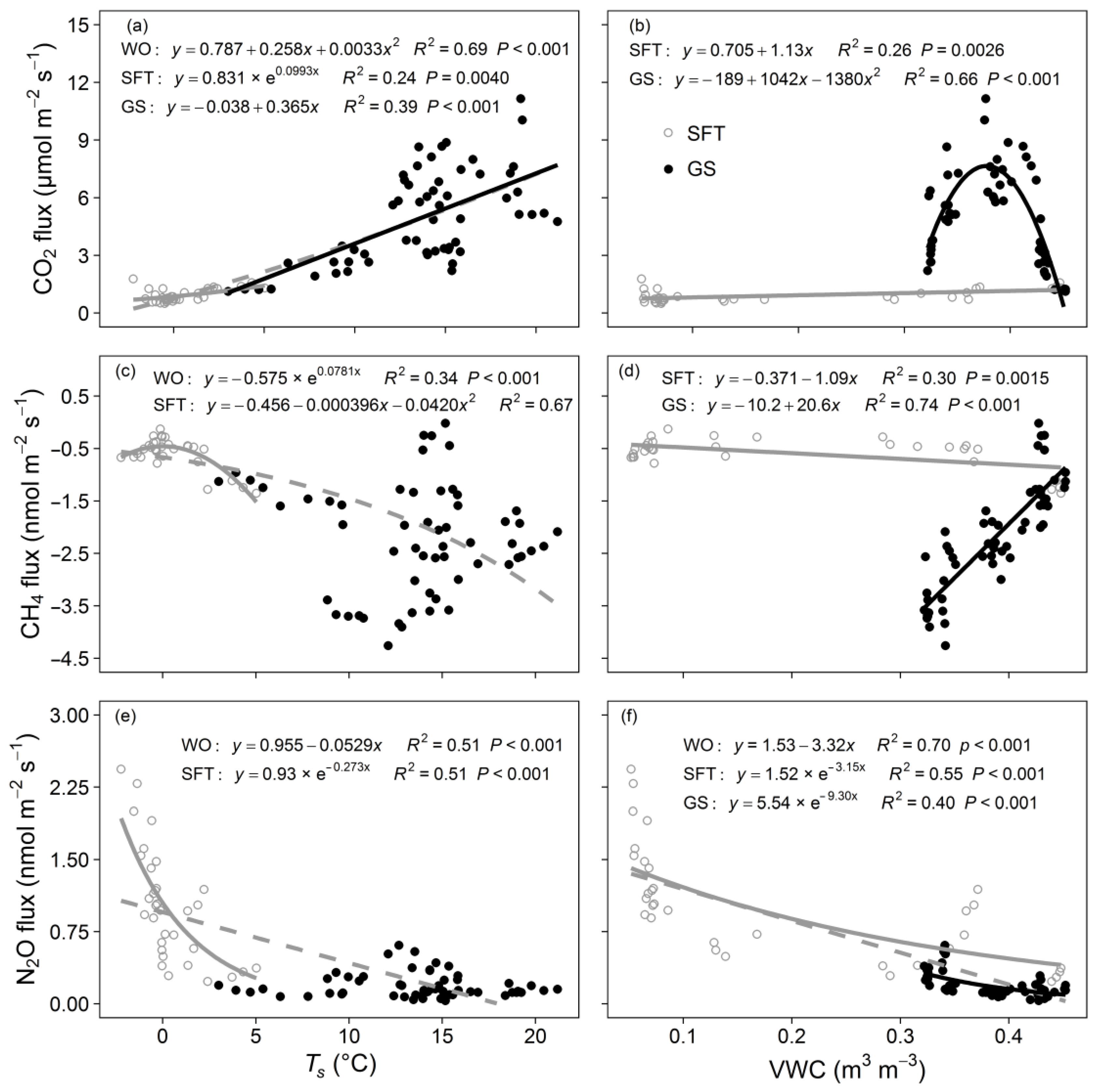
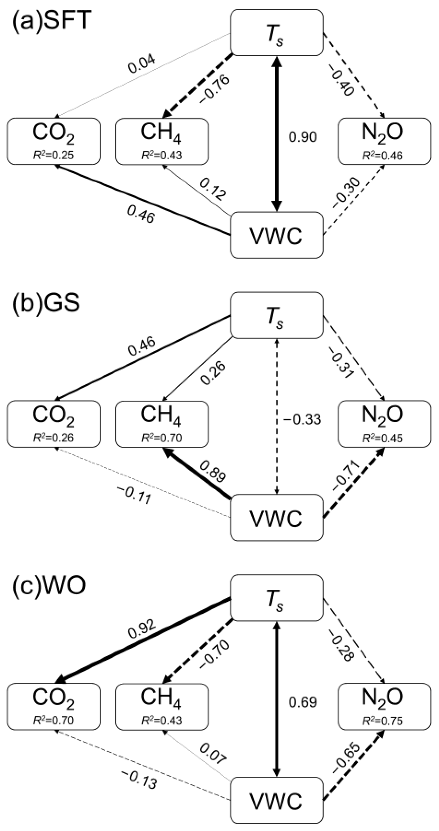
3.4. Responses of Soil CO₂, CH₄, and N₂O Fluxes to Environmental Factors

The responses of CO₂, CH₄, and N₂O fluxes to T_s and VWC during the SFT and GS periods differed (Figure 4). During the WO period, soil CO₂ emissions increased linearly with the increase in T_s (Figure 4a). In general, Q₁₀ is a quotient of the change in R_s by a 10 °C increase in temperature, which indicates the sensitivity of R_s to temperature [55]. The CO₂ emission of the SFT and GS periods had the same sensitivity to T_s, with the same Q₁₀ value of 2.70. However, the response of CO₂ flux to VWC was not significant over the WO period. During the SFT period, the variation range of VWC was large (0.05–0.45 m³ m⁻³); however, the CO₂ flux during this period was relatively low, showing a slow linear upward trend with the increase in VWC. During the GS, CO₂ emissions increased rapidly as VWC increased and then decreased to a low level after the VWC reached 0.38 m³ m⁻³, which can be expressed approximately as a quadratic function (Figure 4b). Path coefficient analysis indicated that both T_s and VWC promoted CO₂ emissions during the SFT period, with a greater contribution of VWC (Figure 5a). Nevertheless, VWC showed a net inhibited CO₂ flux during the GS. In general, the main factor regulating CO₂ emissions during the SFT period was VWC, whereas the main factor controlling CO₂ emission during the GS and WO periods was T_s (Figure 5b,c).

During the WO period, CH₄ uptake increased exponentially with the increase in T_s with a Q₁₀ value of 2.18. Similar to the WO period, CH₄ uptake in the SFT period also increased exponentially with the increase in T_s with a higher Q₁₀ value of 4.53. The CH₄ uptake during the GS increased with the increase in T_s; however, the Q₁₀ value was as low as 1.13. In addition, the effect of T_s on CH₄ was unclear (Figure 4c). Throughout the WO period, the responses of soil CH₄ flux to the changes in VWC distinctly differed between the SFT and GS periods (Figure 4d). During the SFT period, CH₄ uptake decreased linearly with the increase in VWC. Conversely, soil CH₄ uptake during the GS drastically decreased as the VWC increased. However, as the CH₄ uptake was correlated inversely with the VWC during the SFT and GS periods, the response of CH₄ fluxes to the VWC was not significant over the WO period. As shown in the path coefficient analysis (Figure 5), the influences of T_s and VWC on CH₄ uptake during the WO period were consistent with those during the SFT period. Specifically, the CH₄ flux was mainly regulated by T_s during the SFT and WO periods. While during the GS, both T_s and VWC inhibited the uptake of CH₄, and the dominant factor was VWC.

During the SFT period, soil N₂O emissions decreased sharply with the increase of T_s (Figure 4e). The N₂O emissions decreased to approximately 6.7% when T_s increased by 10 °C. In contrast, the N₂O flux did not change significantly with the increase in T_s during the GS (Figure 4e). Consequently, N₂O emission showed a negative correlation to T_s during the WO period with a Q₁₀ value of approximately 0.33, due to the evident negative correlation between the N₂O flux and T_s during the SFT period. During the WO, SFT, and GS periods, the N₂O flux showed a conspicuous downward trend with the increase in VWC (Figure 4f). Overall, T_s and VWC were negatively correlated with N₂O emissions (Figure 5). During the SFT period, N₂O emissions were not only regulated by T_s but also influenced by the VWC. Compared to T_s, VWC had greater control over the N₂O emissions during the GS and WO periods.

3.5. GWP₁₀₀ of Soil CO₂, CH_4, and N₂O Fluxes

The GWP₁₀₀ of these three soil GHG fluxes during the WO period was 37.66 t CO₂ eq ha⁻¹ yr⁻¹. Among three GHGs, soil CO₂ flux contributed to 97.3% of the GWP₁₀₀, followed by N₂O flux (3.1%), whereas CH₄ flux offset 0.4% of the GWP₁₀₀. The GWP₁₀₀ during the GS was 12.54 times higher compared to that during the SFT period, indicating that the GWP₁₀₀ during the GS dominated the GWP₁₀₀ during the WO period.

4. Discussion

4.1. Comparison of Soil GHG Fluxes between the SFT Period and the GS

4.1.1. CO₂

Soil CO₂ flux was relatively stable with low emission during the SFT period, whereas it showed a bimodal pattern during the GS, with higher emission. Low microbial activity limited by the low temperature during the SFT period tended to reduce soil respiration [3]. Compared to the SFT period, the increasing physiological activity of plants during the GS allocated more photosynthetically fixed carbohydrates to roots and microorganisms, which promoted the metabolic activity of the soil microbes to produce CO₂ [71,72].

4.1.2. CH₄

During the WO period, soil acted as a sink for atmospheric CH₄, which is consistent with most previous results [8,32,40,73]. In the present study, the average soil CH₄ flux was −0.50 nmol m⁻² s⁻¹ during the SFT period and −2.24 nmol m⁻² s⁻¹ during the GS (Table 1). At the beginning of the SFT period, the slow decrease in CH₄ uptake may be partly explained by the gradual release of CH₄ from the melting soils, which offsets a portion of the soil CH₄ uptake [22,40]. On the contrary, CH₄ uptake showed an increasing trend at the beginning of the GS, caused by the hydrothermal conditions and aerobic conditions suitable for methanotrophs, together with the inactive methanogenic bacterial community. When entering the rainy season, the soil anaerobic conditions promoted an increase in CH₄ production due to precipitation; therefore, CH₄ uptake was reduced [40].

4.1.3. N₂O

The soil N₂O flux during the SFT period was higher than that in the GS. The pulse emission of soil N₂O detected at the beginning of the SFT period is consistent with the results of Peng et al. [47]. Many studies have reported high soil N₂O emissions during the SFT period in forest ecosystems, which played an important role in regulating the annual N₂O budget [74,75]. For example, N₂O emissions during the FTC accounted for approximately 88% of the annual N₂O emission in a broad-leaved spruce forest in Germany [32]. The average N₂O flux during the SFT period in the present study was 1.15 nmol m⁻² s⁻¹ (Table 1). Studies have found that low temperatures had little influence on the denitrification under anoxic conditions, while net N mineralisation and nitrification within frozen soil could still produce N₂O [34,76]. Thus, a substantial release of N₂O could occur during the soil melting process after a long freezing period [47,77,78]. N₂O emissions showed a gradually decreasing trend during the SFT period (Figure 2). The increasing freeze–thaw cycles gradually consumed the contents of C and N, which lowered the potential of producing N₂O [38]. The N₂O flux during the GS in the present study is approximately three times higher than the average global N₂O flux in temperate forests (0.07 nmol m⁻² s⁻¹) [79]. The possible reasons for the low N₂O flux during the GS may be the substrate limitation caused by the high consumption of substrates during the SFT period and the inhibition of N₂O production caused by the high VWC during this period. At the end of the GS, N₂O emissions tended to increase as precipitation decreased and the soil became dry [80].

4.2. Relationships among Soil GHG Fluxes

The strong coupling effect of soil GHG fluxes increases the uncertainty in estimating the impact of forest soil GHG fluxes on greenhouse effects and global climate change [51,81]. Therefore, it is necessary to observe GHG (CO₂, CH₄, and N₂O) fluxes synchronously. The variation patterns of CO₂ emissions and CH₄ uptake were similar, showing higher fluxes during the GS with two peaks. Under aerobic conditions, the final product of CH₄ oxidation was CO₂, while CH₄ was generated by methanogens under anaerobic conditions by consuming CO₂ [7,82,83]. During the second part of the GS, both the CO₂ emissions and CH₄ uptake were low, which was possibly due to the intensity of precipitation from late June to early August decreased T_s and inhibited soil CO₂ emissions and CH₄ uptake. The decomposition of soil organic matter provided substrates for nitrifying and denitrifying bacteria and promoted the production of soil N₂O flux [84,85]. Soil respiration also affected soil nitrification and denitrification by changing soil aerobic/anaerobic conditions, which consequently affected soil N₂O flux [86]. An evident positive correlation between CH₄ uptake and N₂O emission in the middle of the GS was observed, due to the production or consumption processes related to CH₄ and N₂O fluxes controlled by redox reactions [51,81]. In previous studies, the rates of CH₄ uptake and N₂O emissions were higher under aerobic conditions, and N in the substrate under anaerobic conditions was the common limiting factor that led to a positive correlation between CH₄ uptake and N₂O emissions [81,87].

4.3. Impacts of T_s and Soil VWC on Soil GHG Fluxes

4.3.1. CO₂

T_s generally affected soil respiration by changing soil microbial activities [3,88]. During the GS, T_s was the main driving force of CO₂ emission, with the majority of the CO₂ flux occurred at high T_s. In the present study, the responses of soil CO₂ emissions to soil VWC varied greatly between the SFT and GS periods. The dynamics of soil CO₂ emission was dominated by soil VWC during the SFT period, showing a positive correlation. During the GS, soil CO₂ emissions initially increased and then decreased with the increase in soil VWC, which was consistent with the observation in a mid-temperate forest [34]. In the early stage of the GS, precipitation promoted CO₂ production through increasing available substrates, which was due to the enhanced infiltration of precipitation releasing the previously accumulated CO₂ in the soil pores [89,90]. Soil respiration was sensitive to the intensity and frequency of precipitation. Precipitation events during the early stage of the GS could promote soil CO₂ emissions but had an inverse impact during the late stage of the GS. Soils with higher accumulation of precipitation in the soil pores inhibited the diffusion of soil CO₂ as well as the soil oxygen content, thereby reducing the soil respiration and ultimately resulting in the decreased CO₂ emissions [40,91].

4.3.2. CH₄

Soil CH₄ flux is determined by the balance between methane production from methanogenic archaea and consumption by methanotrophs [7,8,92]. As the aeration condition of forest soil is conducive to methane oxidation [93], forest soils often serve as sinks of CH₄ [8]. The increase in precipitation reduces soil methane uptake by increasing soil VWC [94]. In the present study, CH₄ uptake showed a positive response to T_s (Figure 4). During the SFT period, T_s acted as the main regulator of CH₄ flux. The increase in T_s may stimulate the activity, abundance, and community composition of methanotrophs, thereby promoting CH₄ uptake [50]. In addition, enhanced T_s caused the rise of CH₄ transmission by decreasing soil VWC under warming conditions, thereby enlarging soil pores [25]. A previous study showed that T_s within the range of 5–30 °C had a promoting effect on CH₄ uptake [95], which was consistent with what the present study found during the SFT period. However, no evident correlation between CH₄ uptake and T_s was determined during the GS, which may be related to the strong substrate limitation of methanotrophs [7,40]. It showed that VWC affected soil CH₄ uptake quite differently between the SFT and GS periods. Compared to T_s, soil VWC explained 84% of the variation in the CH₄ flux [96,97]. During the SFT period, CH₄ uptake was generally positively correlated with soil VWC, which may be related to increasingly unstable C and N contents [92]. During the GS, soil VWC played as a key regulator of CH₄ flux and could serve as a good predictor of soil CH₄ uptake. The soil VWC restricted oxygen transmission from the atmosphere to the soil, which reduced methanotroph activity. Meanwhile, soil VWC provided necessary anaerobic conditions for methanogenic bacteria [98,99,100]. Precipitation reduced CH₄ uptake by improving the soil VWC, thereby accelerating the concentration of CH₄ into the atmosphere [94].

4.3.3. N₂O

Previous studies have demonstrated that T_s and soil VWC are key controllers of N₂O emissions in the absence of limitations by other factors. For instance, Kitzler, et al. [101] reported that T_s and soil VWC can explain >95% of the variation in soil N₂O emissions. However, the influence of T_s on N₂O emissions in the present study was more complicated. Soil N₂O emissions showed poor correlation with the variation in T_s during the GS, whereas a higher N₂O emission during the SFT period decreased exponentially with increasing T_s. Soil nitrification is an aerobic process, whereas denitrification is an anaerobic process [102]. Denitrification was the dominant process of N₂O production in soils during the SFT period as the enzyme activity of N₂O production within the denitrification process was not distinctly affected by low temperatures; however, the nitrification process was more inhibited by low temperatures [26,34,103]. This indicates that other factors, such as the reduced amounts of labile substrate availability for microbial metabolism, could be responsible for decreased N₂O emissions with the increase in T_s during the SFT period [33,104]. Soil VWC was the key factor determining the soil N₂O flux during the GS by influencing the N₂O emission inversely. The strict anaerobic condition caused by the limitation of soil oxygen utilisation under high soil VWC triggered the reaction from N₂O to N₂ in the denitrification process, ultimately restricting N₂O emissions [29,105]. Moreover, low microbial activity and N₂O transmission from the soil into the atmosphere under high soil VWC were the inhibited factors for soil N₂O emissions. During the SFT period, N₂O emissions increased drastically. One of the possible reasons was that the soil water molecules expanded after soil freezing, which accelerated the rupture of soil aggregates and subsequently released more soil labile organic matter [40,47]. The labile substrates available for microbial metabolism, which entered different layers of soil with soil water after thawing, were used by the denitrification process to produce N₂O. However, because of substrate supply limitations provided by the nitrification in the microbial denitrifying process, the tremendous increase of N₂O emission is usually discontinuous. On the other hand, nitrification and denitrification are processes that depend on suitable oxygen availability that produces N₂O [8]. Nevertheless, the soil N₂O flux decreased during the late stage of the SFT period caused by the decrease in oxygen concentrations due to the increasing soil VWC. Conversely, the variation trend of soil N₂O emissions was consistent with the WWC trend. The reason may be that the frozen water content of soil rapidly decreased, which only distinctly affected soil WWC, whereas the available water content in soil (VWC) rapidly increased during the SFT period.

4.4. Contributions of Soil GHG Fluxes to the Greenhouse Effect

Determining the GWP₁₀₀ of forest soil CO₂, CH₄, and N₂O fluxes would help assess the impacts of soil GHG exchanges on global warming [106]. In the present study, there were distinct differences in GWP₁₀₀ of the temperate forest soil between the SFT and GS periods; the GWP₁₀₀ during the GS was approximately 12.54 times higher than that during the SFT period. The soil GHG fluxes during the GS were of greater significance to global warming due to the higher rates and total amounts of CO₂ flux in this period; the GWP₁₀₀ of the CO₂ flux was 32,170.84 kg CO₂ eq ha⁻¹ yr⁻¹ during the GS and 1870.22 kg CO₂ eq ha⁻¹ yr⁻¹ during the SFT period. Similar results have been found in previous studies, where the CO₂ flux contributed >90% of the GWP₁₀₀ [51,55]. Although the CO₂ flux made the largest contribution to GWP₁₀₀, the warming capacities of CH₄ and N₂O are much stronger than that of CO₂ [2]. Compared to the GS, the SFT period had higher N₂O emissions and lower CH₄ uptake, and therefore, their GWP₁₀₀ values during the SFT period cannot be ignored. The GWP₁₀₀ of the N₂O flux during the SFT period (723.05 kg CO₂ eq ha⁻¹ yr⁻¹) contributed more than that during the GS (348.95 kg CO₂ eq ha⁻¹ yr⁻¹), whereas the GWP₁₀₀ of the CH₄ flux during the SFT period (−9.60 kg CO₂ eq ha⁻¹ yr⁻¹) offset less than the GWP₁₀₀ during the GS (−122.04 kg CO₂ eq ha⁻¹ yr⁻¹). The GWP₁₀₀ of CH₄ ( −0.12 t CO₂ eq ha⁻¹ yr⁻¹) for the over-mature forest in Northeastern China was close to that found in the present study [55]. While the GWP₁₀₀ of N₂O (1.63 t CO₂ eq ha⁻¹ yr⁻¹) in Wu and Mu [55] was higher than that reported in this present study, which was mainly due to the spatial heterogeneity of the N₂O flux. In addition, the mean N₂O flux during the SFT period in the results of Peng et al. [47] (2.16 nmol m^-2 s^-1) was higher than that during the same period (1.15 nmol m^-2 s^-1) in this study. Due to the high soil N₂O emissions during the FTCs in the temperate forest, the incomplete non-growing season observation of GHG fluxes in the present study led to the underestimation of the GWP₁₀₀ of the N₂O flux [34,47,78].

5. Conclusions

Overall, we comprehensively examined the soil GHG (CO₂, CH₄, and N₂O) fluxes between the SFT and GS periods in a temperate broad-leaved Korean pine mixed forest and investigated their connections with the major environmental variables (T_s and soil VWC). Our results indicate that the cumulative fluxes of both CO₂ emissions and CH₄ uptake during the GS were far higher than those during the SFT period. However, the cumulative N₂O fluxes in the SFT period accounted for 64.7% of the total emissions in the WO period, which was probably attributed to a substantial release of N₂O after a long freezing period and the decomposition of soil nitrification and denitrification resulted from the increased soil microbial activities and available substrates during the SFT period. Furthermore, CO₂ emissions and CH₄ uptake showed similar variation trends throughout the WO period. Meanwhile, N₂O emissions and CH₄ uptake presented consistent variation trends during most of the GS. These results imply that the effect of T_s and soil VWC on the mechanisms of soil GHG emissions/uptake can be similar in certain periods throughout the year.

Affected by the East-Asia monsoon climate, the T_s and soil VWC in this temperate forest differed drastically between the SFT and GS periods. We found that soil GHG fluxes responded differently to T_s and soil VWC during the SFT and GS periods. N₂O emissions decreased drastically with the increases in T_s and soil VWC during the SFT period but varied little with T_s during the GS. While soil N₂O emissions and CH₄ uptake were dominated by the soil VWC during the GS, soil CO₂ emissions and CH₄ uptake during the WO period were mainly controlled by the T_s. These results stress the role of T_s and soil VWC in shaping soil GHG fluxes during the SFT and GS periods, respectively, thereby helping to improve the accuracy in estimating the soil GHG budgets under global climate change.

The results also show that soil CO₂ flux contributed predominantly for GWP₁₀₀ followed by soil N₂O flux, whereas soil CH₄ flux was an offsetting factor for the total GWP₁₀₀. Taken together, our findings suggest that the soil freeze–thaw cycle is important to characterise the dynamics of soil GHG fluxes and highlight the importance of the N₂O pulse during the SFT period. Further studies are required for the exploration of the mechanisms among soil GHG exchanges and the accurate estimation of total annual GHG fluxes and their global warming potential by analysing soil GHG fluxes, soil properties, and soil microbial characteristics in a longer time series, especially during the SFT period.

References

1. Kirschbaum, M.U.F. Will changes in soil organic carbon act as a positive or negative feedback on global warming? Biogeochemistry 2000, 48, 21–51. [Google Scholar] [CrossRef]
2. IPCC. Climate Change 2013: The Physical Science Basis. Contribution of Working Group I to the Fifth Assessment Report of the Intergovernmental Panel on Climate Change; Cambridge University Press: Cambridge, UK; New York, NY, USA, 2013; p. 1535. [Google Scholar]
3. Lloyd, J.; Taylor, J.A. On the Temperature Dependence of Soil Respiration. Funct. Ecol. 1994, 8, 315–323. [Google Scholar] [CrossRef]
4. Fuglestvedt, J.S.; Berntsen, T.K.; Godal, O.; Skodvin, T. Climate implications of GWP-based reductions in greenhouse gas emissions. Geophys. Res. Lett. 2000, 27, 409–412. [Google Scholar] [CrossRef]
5. Le Treut, H.; Somerville, R. Chapter 1: Historical overview of climate change science. In IPCC Fourth Assessment Review: Climate Change Science; Cambridge University Press: Cambridge, UK; New York, NY, USA, 2007. [Google Scholar]
6. Oertel, C.; Matschullat, J.; Zurba, K.; Zimmermann, F.; Erasmi, S. Greenhouse gas emissions from soils—A review. Geochemistry 2016, 76, 327–352. [Google Scholar] [CrossRef] [Green Version]
7. Feng, H.; Guo, J.; Han, M.; Wang, W.; Peng, C.; Jin, J.; Song, X.; Yu, S. A review of the mechanisms and controlling factors of methane dynamics in forest ecosystems. For. Ecol. Manag. 2020, 455, 117702. [Google Scholar] [CrossRef]
8. Sa, M.M.F.; Schaefer, C.; Loureiro, D.C.; Simas, F.N.B.; Alves, B.J.R.; de Sa Mendonca, E.; de Figueiredo, E.B.; La Scala, N., Jr.; Panosso, A.R. Fluxes of CO2, CH4, and N2O in tundra-covered and Nothofagus forest soils in the Argentinian Patagonia. Sci. Total Environ. 2019, 659, 401–409. [Google Scholar] [CrossRef] [PubMed]
9. Lal, R. Forest soils and carbon sequestration. For. Ecol. Manag. 2005, 220, 242–258. [Google Scholar] [CrossRef]
10. Dixon, R.K. Carbon pools and flux of global forest ecosystems (Vol 263, Pg 185, 1994). Science 1994, 265, 171. [Google Scholar]
11. Cole, D.W.; Rapp, M. Elemental cycling in forest ecosystems. In Dynamic Properties of Forest Ecosystems; Reichle, D.E., Ed.; Cambridge University Press: Cambridge, UK, 2009; pp. 341–375. [Google Scholar]
12. Huang, G.; Li, Y.; Su, Y.G. Effects of increasing precipitation on soil microbial community composition and soil respiration in a temperate desert, Northwestern China. Soil Biol. Biochem. 2015, 83, 52–56. [Google Scholar] [CrossRef]
13. Davidson, E.A.; Belk, E.; Boone, R.D. Soil water content and temperature as independent or confounded factors controlling soil respiration in a temperate mixed hardwood forest. Glob. Chang. Biol. 1998, 4, 217–227. [Google Scholar] [CrossRef] [Green Version]
14. Högberg, P.; Nordgren, A.; Buchmann, N.; Taylor, A.F.S.; Ekblad, A.; Högberg, M.N.; Nyberg, G.; Ottosson-Löfvenius, M.; Read, D.J. Large-scale forest girdling shows that current photosynthesis drives soil respiration. Nature 2001, 411, 789–792. [Google Scholar] [CrossRef]
15. Luo, G.J.; Kiese, R.; Wolf, B.; Butterbach-Bahl, K. Effects of soil temperature and moisture on methane uptake and nitrous oxide emissions across three different ecosystem types. Biogeosciences 2013, 10, 3205–3219. [Google Scholar] [CrossRef] [Green Version]
16. Liu, L.; Estiarte, M.; Penuelas, J. Soil moisture as the key factor of atmospheric CH4 uptake in forest soils under environmental change. Geoderma 2019, 355, 113920. [Google Scholar] [CrossRef]
17. Petrakis, S.; Seyfferth, A.; Kan, J.; Inamdar, S.; Vargas, R. Influence of experimental extreme water pulses on greenhouse gas emissions from soils. Biogeochemistry 2017, 133, 147–164. [Google Scholar] [CrossRef]
18. Butterbach-Bahl, K.; Baggs, E.M.; Dannenmann, M.; Kiese, R.; Zechmeister-Boltenstern, S. Nitrous oxide emissions from soils: How well do we understand the processes and their controls? Philos. Trans. R. Soc. B Biol. Sci. 2013, 368, 20130122. [Google Scholar] [CrossRef]
19. Müller, C.; Martin, M.; Stevens, R.J.; Laughlin, R.J.; Kammann, C.; Ottow, J.C.G.; Jäger, H.J. Processes leading to N2O emissions in grassland soil during freezing and thawing. Soil Biol. Biochem. 2002, 34, 1325–1331. [Google Scholar] [CrossRef]
20. McCalley, C.K.; Woodcroft, B.J.; Hodgkins, S.B.; Wehr, R.A.; Kim, E.H.; Mondav, R.; Crill, P.M.; Chanton, J.P.; Rich, V.I.; Tyson, G.W.; et al. Methane dynamics regulated by microbial community response to permafrost thaw. Nature 2014, 514, 478–481. [Google Scholar] [CrossRef] [Green Version]
21. Fang, Y.; Gundersen, P.; Zhang, W.; Zhou, G.; Christiansen, J.R.; Mo, J.; Dong, S.; Zhang, T. Soil–atmosphere exchange of N2O, CO2 and CH4 along a slope of an evergreen broad-leaved forest in southern China. Plant Soil 2009, 319, 37–48. [Google Scholar] [CrossRef]
22. Curiel Yuste, J.; Baldocchi, D.D.; Gershenson, A.; Goldstein, A.; Misson, L.; Wong, S. Microbial soil respiration and its dependency on carbon inputs, soil temperature and moisture. Glob. Chang. Biol. 2007, 13, 2018–2035. [Google Scholar] [CrossRef] [Green Version]
23. Tu, C.; Li, F.D. Responses of greenhouse gas fluxes to experimental warming in wheat season under conventional tillage and no-tillage fields. J. Environ. Sci. 2017, 54, 314–327. [Google Scholar] [CrossRef]
24. Zang, H.; Blagodatskaya, E.; Wen, Y.; Shi, L.; Cheng, F.; Chen, H.; Zhao, B.; Zhang, F.; Fan, M.; Kuzyakov, Y. Temperature sensitivity of soil organic matter mineralization decreases with long-term N fertilization: Evidence from four Q10 estimation approaches. Land Degrad. Dev. 2020, 31, 683–693. [Google Scholar] [CrossRef]
25. Dijkstra, F.A.; Prior, S.A.; Runion, G.B.; Torbert, H.A.; Tian, H.; Lu, C.; Venterea, R.T. Effects of elevated carbon dioxide and increased temperature on methane and nitrous oxide fluxes: Evidence from field experiments. Front. Ecol. Environ. 2012, 10, 520–527. [Google Scholar] [CrossRef]
26. Wu, X.; Wang, F.; Li, T.; Fu, B.; Lv, Y.; Liu, G. Nitrogen additions increase N2O emissions but reduce soil respiration and CH4 uptake during freeze–thaw cycles in an alpine meadow. Geoderma 2020, 363, 114157. [Google Scholar] [CrossRef]
27. Blankinship, J.C.; Brown, J.R.; Dijkstra, P.; Allwright, M.C.; Hungate, B.A. Response of Terrestrial CH4 Uptake to Interactive Changes in Precipitation and Temperature Along a Climatic Gradient. Ecosystems 2010, 13, 1157–1170. [Google Scholar] [CrossRef]
28. Sponseller, R.A. Precipitation pulses and soil CO2 flux in a Sonoran Desert ecosystem. Glob. Chang. Biol. 2007, 13, 426–436. [Google Scholar] [CrossRef]
29. Wen, Y.; Zang, H.; Freeman, B.; Ma, Q.; Chadwick, D.R.; Jones, D.L. Rye cover crop incorporation and high watertable mitigate greenhouse gas emissions in cultivated peatland. Land Degrad. Dev. 2019, 30, 1928–1938. [Google Scholar] [CrossRef]
30. Carey, J.C.; Tang, J.W.; Templer, P.H.; Kroeger, K.D.; Crowther, T.W.; Burton, A.J.; Dukes, J.S.; Emmett, B.; Frey, S.D.; Heskel, M.A.; et al. Temperature response of soil respiration largely unaltered with experimental warming. Proc. Natl. Acad. Sci. USA 2016, 113, 13797–13802. [Google Scholar] [CrossRef] [Green Version]
31. Fang, C.; Moncrieff, J.B. The dependence of soil CO2 efflux on temperature. Soil Biol. Biochem. 2001, 33, 155–165. [Google Scholar] [CrossRef]
32. Luo, G.J.; Brüggemann, N.; Wolf, B.; Gasche, R.; Grote, R.; Butterbach-Bahl, K. Decadal variability of soil CO2, NO, N2O, and CH4 fluxes at the Höglwald Forest, Germany. Biogeosciences 2012, 9, 1741–1763. [Google Scholar] [CrossRef] [Green Version]
33. Zou, J.; Tobin, B.; Luo, Y.; Osborne, B. Differential responses of soil CO2 and N2O fluxes to experimental warming. Agric. For. Meteorol. 2018, 259, 11–22. [Google Scholar] [CrossRef]
34. Gao, D.; Zhang, L.; Liu, J.; Peng, B.; Fan, Z.; Dai, W.; Jiang, P.; Bai, E. Responses of terrestrial nitrogen pools and dynamics to different patterns of freeze-thaw cycle: A meta-analysis. Glob. Chang. Biol. 2018, 24, 2377–2389. [Google Scholar] [CrossRef] [PubMed]
35. Chen, Z.; Yang, S.-q.; Zhang, A.-p.; Jing, X.; Song, W.-m.; Mi, Z.-r.; Zhang, Q.-w.; Wang, W.-y.; Yang, Z.-l. Nitrous oxide emissions following seasonal freeze-thaw events from arable soils in Northeast China. J. Integr. Agric. 2018, 17, 231–246. [Google Scholar] [CrossRef]
36. Zhang, T.; Barry, R.; Knowles, K.; Ling, F.; Armstrong, R. Distribution of seasonally and perennially frozen ground in the Northern Hemisphere. In Proceedings of the 8th International Conference on Permafrost, Zürich, Switzerland, 21–25 July 2003; Volume 2. [Google Scholar]
37. Wang, C.; Han, Y.; Chen, J.; Wang, X.; Zhang, Q.; Bond-Lamberty, B. Seasonality of soil CO2 efflux in a temperate forest: Biophysical effects of snowpack and spring freeze–thaw cycles. Agric. For. Meteorol. 2013, 177, 83–92. [Google Scholar] [CrossRef]
38. Han, C.; Gu, Y.; Kong, M.; Hu, L.; Jia, Y.; Li, F.; Sun, G.; Siddique, K.H.M. Responses of soil microorganisms, carbon and nitrogen to freeze–thaw cycles in diverse land-use types. Appl. Soil Ecol. 2018, 124, 211–217. [Google Scholar] [CrossRef]
39. Song, Y.; Zou, Y.; Wang, G.; Yu, X. Altered soil carbon and nitrogen cycles due to the freeze-thaw effect: A meta-analysis. Soil Biol. Biochem. 2017, 109, 35–49. [Google Scholar] [CrossRef]
40. Kim, D.G.; Vargas, R.; Bond-Lamberty, B.; Turetsky, M.R. Effects of soil rewetting and thawing on soil gas fluxes: A review of current literature and suggestions for future research. Biogeosci. Discuss. 2011, 8, 9847–9899. [Google Scholar] [CrossRef]
41. Wagner-Riddle, C.; Congreves, K.A.; Abalos, D.; Berg, A.A.; Brown, S.E.; Ambadan, J.T.; Gao, X.; Tenuta, M. Globally important nitrous oxide emissions from croplands induced by freeze–thaw cycles. Nat. Geosci. 2017, 10, 279–283. [Google Scholar] [CrossRef]
42. Mastepanov, M.; Sigsgaard, C.; Dlugokencky, E.J.; Houweling, S.; Ström, L.; Tamstorf, M.P.; Christensen, T.R. Large tundra methane burst during onset of freezing. Nature 2008, 456, 628–630. [Google Scholar] [CrossRef] [Green Version]
43. Kurganova, I.; Teepe, R.; Loftfield, N. Influence of freeze-thaw events on carbon dioxide emission from soils at different moisture and land use. Carbon Balance Manag. 2007, 2, 2. [Google Scholar] [CrossRef] [Green Version]
44. Wu, G.; Chen, X.-M.; Ling, J.; Li, F.; Li, F.-Y.; Peixoto, L.; Wen, Y.; Zhou, S.-L. Effects of soil warming and increased precipitation on greenhouse gas fluxes in spring maize seasons in the North China Plain. Sci. Total Environ. 2020, 734, 139269. [Google Scholar] [CrossRef]
45. Cooper, M.D.A.; Estop-Aragonés, C.; Fisher, J.P.; Thierry, A.; Garnett, M.H.; Charman, D.J.; Murton, J.B.; Phoenix, G.K.; Treharne, R.; Kokelj, S.V.; et al. Limited contribution of permafrost carbon to methane release from thawing peatlands. Nat. Clim. Chang. 2017, 7, 507–511. [Google Scholar] [CrossRef]
46. Congreves, K.A.; Wagner-Riddle, C.; Si, B.C.; Clough, T.J. Nitrous oxide emissions and biogeochemical responses to soil freezing-thawing and drying-wetting. Soil Biol. Biochem. 2018, 117, 5–15. [Google Scholar] [CrossRef]
47. Peng, B.; Sun, J.; Liu, J.; Dai, W.; Sun, L.; Pei, G.; Gao, D.; Wang, C.; Jiang, P.; Bai, E. N2O emission from a temperate forest soil during the freeze-thaw period: A mesocosm study. Sci. Total Environ. 2019, 648, 350–357. [Google Scholar] [CrossRef] [PubMed]
48. Guan, D.; Wu, J.; Zhao, X.; Han, S.; Yu, G.; Sun, X.; Jin, C. CO2 fluxes over an old, temperate mixed forest in northeastern China. Agric. For. Meteorol. 2006, 137, 138–149. [Google Scholar] [CrossRef]
49. Yu, G.; Zhang, L.; Sun, X.; Fu, Y.; Wen, X.; Wang, Q.; Li, S.; Ren, C.; Song, X.; Liu, Y.; et al. Environmental controls over carbon exchange of three forest ecosystems in eastern China. Glob. Chang. Biol. 2008, 14, 2555–2571. [Google Scholar] [CrossRef]
50. Zhou, Y.; Hagedorn, F.; Zhou, C.; Jiang, X.; Wang, X.; Li, M.-H. Experimental warming of a mountain tundra increases soil CO2 effluxes and enhances CH4 and N2O uptake at Changbai Mountain, China. Sci. Rep. 2016, 6, 21108. [Google Scholar] [CrossRef] [Green Version]
51. Chen, Z.; Setälä, H.; Geng, S.; Han, S.; Wang, S.; Dai, G.; Zhang, J. Nitrogen addition impacts on the emissions of greenhouse gases depending on the forest type: A case study in Changbai Mountain, Northeast China. J. Soils Sediments 2017, 17, 23–34. [Google Scholar] [CrossRef] [Green Version]
52. Wang, M.; Guan, D.-X.; Han, S.-J.; Wu, J.-L. Comparison of eddy covariance and chamber-based methods for measuring CO2 flux in a temperate mixed forest. Tree Physiol. 2009, 30, 149–163. [Google Scholar] [CrossRef] [Green Version]
53. Wu, J.; Guan, D.; Wang, M.; Pei, T.; Han, S.; Jin, C. Year-round soil and ecosystem respiration in a temperate broad-leaved Korean Pine forest. For. Ecol. Manag. 2006, 223, 35–44. [Google Scholar] [CrossRef]
54. Bai, E.; Li, W.; Li, S.; Sun, J.; Peng, B.; Dai, W.; Jiang, P.; Han, S. Pulse increase of soil N2O emission in response to N addition in a temperate forest on Mt Changbai, northeast China. PLoS ONE 2014, 9, e102765. [Google Scholar] [CrossRef]
55. Wu, B.; Mu, C.C. Effects on Greenhouse Gas (CH4, CO2, N2O) Emissions of Conversion from Over-Mature Forest to Secondary Forest and Korean Pine Plantation in Northeast China. Forests 2019, 10, 788. [Google Scholar] [CrossRef] [Green Version]
56. Phillips, S.C.; Varner, R.K.; Frolking, S.; Munger, J.W.; Bubier, J.L.; Wofsy, S.C.; Crill, P.M. Interannual, seasonal, and diel variation in soil respiration relative to ecosystem respiration at a wetland to upland slope at Harvard Forest. J. Geophys. Res. Biogeosci. 2010, 115. [Google Scholar] [CrossRef]
57. Wan, Q.; Feng, X.; Lu, J.; Zheng, W.; Song, X.; Li, P.; Han, S.; Xu, H. Atmospheric mercury in Changbai Mountain area, northeastern China II. The distribution of reactive gaseous mercury and particulate mercury and mercury deposition fluxes. Environ. Res. 2009, 109, 721–727. [Google Scholar] [CrossRef]
58. Wang, Z.; Gallet, J.; Pedersen, C.; Zhang, X.; Ström, J.; Ci, Z. Elemental carbon in snow at Changbai Mountain, northeastern China: Concentrations, scavenging ratios, and dry deposition velocities. Atmos. Chem. Phys. 2014, 14. [Google Scholar] [CrossRef] [Green Version]
59. FAO. World Reference Base for Soil Resources 2014: International Soil Classification System for Naming Soils and Creating Legends for Soil Maps; World Soil Resources Reports No. 106; FAO: Rome, Italy, 2015. [Google Scholar]
60. Hao, Z.; Zhang, J.; Song, B.; Ye, J.; Li, B. Vertical structure and spatial associations of dominant tree species in an old-growth temperate forest. For. Ecol. Manag. 2007, 252, 1–11. [Google Scholar] [CrossRef]
61. Zheng, X.; Mei, B.; Wang, Y.; Xie, B.; Wang, Y.; Dong, H.; Xu, H.; Chen, G.; Cai, Z.; Yue, J.; et al. Quantification of N2O fluxes from soil–plant systems may be biased by the applied gas chromatograph methodology. Plant Soil 2008, 311, 211–234. [Google Scholar] [CrossRef]
62. Liu, J.; Chen, H.; Yang, X.; Gong, Y.; Zheng, X.; Fan, M.; Kuzyakov, Y. Annual methane uptake from different land uses in an agro-pastoral ecotone of northern China. Agric. For. Meteorol. 2017, 236, 67–77. [Google Scholar] [CrossRef]
63. Zheng, Z.M.; Yu, G.R.; Sun, X.M.; Li, S.G.; Wang, Y.S.; Wang, Y.H.; Fu, Y.L.; Wang, Q.F. Spatio-temporal variability of soil respiration of forest ecosystems in China: Influencing factors and evaluation model. Environ. Manag. 2010, 46, 633–642. [Google Scholar] [CrossRef]
64. Yang, X.; Chen, H.; Gong, Y.; Zheng, X.; Fan, M.; Kuzyakov, Y. Nitrous oxide emissions from an agro-pastoral ecotone of northern China depending on land uses. Agric. Ecosyst. Environ. 2015, 213, 241–251. [Google Scholar] [CrossRef]
65. Streiner, D.L. Maintaining Standards: Differences between the Standard Deviation and Standard Error, and When to Use Each. Can. J. Psychiatry 1996, 41, 498–502. [Google Scholar] [CrossRef]
66. Brinkmann, W.A.R. Growing season length as an indicator of climatic variations? Clim. Chang. 1979, 2, 127–138. [Google Scholar] [CrossRef]
67. Segura, J.H.; Nilsson, M.B.; Haei, M.; Sparrman, T.; Mikkola, J.P.; Grasvik, J.; Schleucher, J.; Oquist, M.G. Microbial mineralization of cellulose in frozen soils. Nat. Commun. 2017, 8, 1154. [Google Scholar] [CrossRef] [PubMed] [Green Version]
68. Brooks, P.D.; Grogan, P.; Templer, P.H.; Groffman, P.; Öquist, M.G.; Schimel, J. Carbon and Nitrogen Cycling in Snow-Covered Environments. Geogr. Compass 2011, 5, 682–699. [Google Scholar] [CrossRef]
69. Arslantaş, E.E.; Yeşilırmak, E. Changes in the climatic growing season in western Anatolia, Turkey. Meteorol. Appl. 2020, 27, e1897. [Google Scholar] [CrossRef]
70. Kunkel, K.E.; Easterling, D.R.; Hubbard, K.; Redmond, K. Temporal variations in frost-free season in the United States: 1895–2000. Geophys. Res. Lett. 2004, 31. [Google Scholar] [CrossRef]
71. Raich, J.W.; Potter, C.S.; Bhagawati, D. Interannual variability in global soil respiration, 1980–94. Glob. Chang. Biol. 2002, 8, 800–812. [Google Scholar] [CrossRef]
72. Raich, J.W.; Potter, C.S. Global patterns of carbon dioxide emissions from soils. Glob. Biogeochem. Cycles 1995, 9, 23–36. [Google Scholar] [CrossRef] [Green Version]
73. Dong, Y.; Scharffe, D.; Lobert, J.M.; Crutzen, P.J.; Sanhueza, E. Fluxes of CO2, CH4 and N2O from a temperate forest soil: The effects of leaves and humus layers. Tellus B 1998, 50, 243–252. [Google Scholar] [CrossRef]
74. Wu, X.; Brüggemann, N.; Gasche, R.; Shen, Z.; Wolf, B.; Butterbach-Bahl, K. Environmental controls over soil-atmosphere exchange of N2O, NO, and CO2 in a temperate Norway spruce forest. Glob. Biogeochem. Cycles 2010, 24. [Google Scholar] [CrossRef]
75. Guckland, A.; Corre, M.D.; Flessa, H. Variability of soil N cycling and N2O emission in a mixed deciduous forest with different abundance of beech. Plant Soil 2010, 336, 25–38. [Google Scholar] [CrossRef] [Green Version]
76. Smith, J.; Wagner-Riddle, C.; Dunfield, K. Season and management related changes in the diversity of nitrifying and denitrifying bacteria over winter and spring. Appl. Soil Ecol. 2010, 44, 138–146. [Google Scholar] [CrossRef]
77. Öquist, M.G.; Nilsson, M.; Sörensson, F.; Kasimir-Klemedtsson, Å.; Persson, T.; Weslien, P.; Klemedtsson, L. Nitrous oxide production in a forest soil at low temperatures – processes and environmental controls. FEMS Microbiol. Ecol. 2004, 49, 371–378. [Google Scholar] [CrossRef] [PubMed]
78. Goldberg, S.D.; Borken, W.; Gebauer, G. N2O emission in a Norway spruce forest due to soil frost: Concentration and isotope profiles shed a new light on an old story. Biogeochemistry 2010, 97, 21–30. [Google Scholar] [CrossRef]
79. Dalal, R.; Allen, D. Greenhouse gas fluxes from natural ecosystems. Aust. J. Bot. 2008, 56, 396–407. [Google Scholar] [CrossRef]
80. Xing, G.X.; Zhu, Z.L. Preliminary studies on N2O emission fluxes from upland soils and paddy soils in China. Nutr. Cycl. Agroecosyst. 1997, 49, 17–22. [Google Scholar] [CrossRef]
81. Zhang, X.; Xu, H.; Chen, G. Major factors controlling nitrous oxide emission and methane uptake from forest soil. J. For. Res. 2001, 12, 239–242. [Google Scholar] [CrossRef]
82. Ferry, J.G. Methane: Small molecule, big impact. Science 1997, 278, 1413–1414. [Google Scholar] [CrossRef]
83. Whalen, S.C.; Reeburgh, W.S. Methane oxidation, production, and emission at contrasting sites in a boreal bog. Geomicrobiol. J. 2000, 17, 237–251. [Google Scholar]
84. Garcia-Montiel, D.; Melillo, J.; Steudler, P.A.; Cerri, C.C.; Piccolo, M.C. Carbon limitations to nitrous oxide emissions in a humid tropical forest of the Brazilian Amazon. Biol. Fertil. Soils 2003, 38, 267–272. [Google Scholar] [CrossRef]
85. Kettunen, R.; Saarnio, S.; Martikainen, P.J.; Silvola, J. Can a mixed stand of N2-fixing and non-fixing plants restrict N2O emissions with increasing CO2 concentration? Soil Biol. Biochem. 2007, 39, 2538–2546. [Google Scholar] [CrossRef]
86. Azam, F.; Gill, S.; Farooq, S. Availability of CO2 as a factor affecting the rate of nitrification in soil. Soil Biol. Biochem. 2005, 37, 2141–2144. [Google Scholar] [CrossRef]
87. Megmw, S.; Knowles, R. Active methanotrophs suppress nitrification in a humisol. Biol. Fertil. Soils 1987, 4, 205–212. [Google Scholar] [CrossRef]
88. Zhou, J.; Zang, H.; Loeppmann, S.; Gube, M.; Kuzyakov, Y.; Pausch, J. Arbuscular mycorrhiza enhances rhizodeposition and reduces the rhizosphere priming effect on the decomposition of soil organic matter. Soil Biol. Biochem. 2020, 140, 107641. [Google Scholar] [CrossRef]
89. Huxman, T.E.; Snyder, K.A.; Tissue, D.; Leffler, A.J.; Ogle, K.; Pockman, W.T.; Sandquist, D.R.; Potts, D.L.; Schwinning, S. Precipitation pulses and carbon fluxes in semiarid and arid ecosystems. Oecologia 2004, 141, 254–268. [Google Scholar] [CrossRef]
90. Stark, J.M.; Firestone, M.K. Mechanisms for soil moisture effects on activity of nitrifying bacteria. Appl. Environ. Microbiol. 1995, 61, 218–221. [Google Scholar] [CrossRef] [Green Version]
91. Gao, D.; Hagedorn, F.; Zhang, L.; Liu, J.; Qu, G.; Sun, J.; Peng, B.; Fan, Z.; Zheng, J.; Jiang, P.; et al. Small and transient response of winter soil respiration and microbial communities to altered snow depth in a mid-temperate forest. Appl. Soil Ecol. 2018, 130, 40–49. [Google Scholar] [CrossRef]
92. Wu, H.; Xu, X.; Duan, C.; Li, T.; Cheng, W. Synergistic effects of dissolved organic carbon and inorganic nitrogen on methane uptake in forest soils without and with freezing treatment. Sci. Rep. 2016, 6, 32555. [Google Scholar] [CrossRef]
93. Gulledge, J.; Hrywna, Y.; Cavanaugh, C.; Steudler, P.A. Effects of long-term nitrogen fertilization on the uptake kinetics of atmospheric methane in temperate forest soils. FEMS Microbiol. Ecol. 2004, 49, 389–400. [Google Scholar] [CrossRef]
94. Ni, X.; Groffman, P.M. Declines in methane uptake in forest soils. Proc. Natl. Acad. Sci. USA 2018, 115, 8587–8590. [Google Scholar] [CrossRef] [Green Version]
95. Macdonald, J.A.; Eggleton, P.; Bignell, D.E.; Forzi, F.; Fowler, D. Methane emission by termites and oxidation by soils, across a forest disturbance gradient in the Mbalmayo Forest Reserve, Cameroon. Glob. Chang. Biol. 1998, 4, 409–418. [Google Scholar] [CrossRef]
96. Sgouridis, F.; Ullah, S. Soil greenhouse gas fluxes, environmental controls, and the partitioning of N2O sources in UK natural and seminatural land use types. J. Geophys. Res. Biogeosci. 2017, 122, 2617–2633. [Google Scholar] [CrossRef]
97. Borken, W.; Davidson, E.A.; Savage, K.; Sundquist, E.T.; Steudler, P. Effect of summer throughfall exclusion, summer drought, and winter snow cover on methane fluxes in a temperate forest soil. Soil Biol. Biochem. 2006, 38, 1388–1395. [Google Scholar] [CrossRef]
98. Gao, B.; Ju, X.; Su, F.; Meng, Q.; Oenema, O.; Christie, P.; Chen, X.; Zhang, F. Nitrous oxide and methane emissions from optimized and alternative cereal cropping systems on the North China Plain: A two-year field study. Sci. Total Environ. 2014, 472, 112–124. [Google Scholar] [CrossRef]
99. Song, W.; Wang, H.; Guangshuai, W.; Chen, L.; Jin, Z.; Zhuang, Q.; He, J.-S. Methane emissions from an alpine wetland on the Tibetan Plateau: Neglected but vital contribution of non-growing season. J. Geophys. Res. Biogeosci. 2015. [Google Scholar] [CrossRef]
100. Granberg, G.; Ottosson-Löfvenius, M.; Grip, H.; Sundh, I.; Nilsson, M. Effect of climatic variability from 1980 to 1997 on simulated methane emission from a boreal mixed mire in northern Sweden. Glob. Biogeochem. Cycles 2001, 15, 977–991. [Google Scholar] [CrossRef]
101. Kitzler, B.; Zechmeister-Boltenstern, S.; Holtermann, C.; Skiba, U.; Butterbach-Bahl, K. Nitrogen oxides emission from two beech forests subjected to different nitrogen loads. Biogeosciences 2006, 3, 293–310. [Google Scholar] [CrossRef] [Green Version]
102. Braker, G.; Conrad, R. Chapter 2—Diversity, Structure, and Size of N2O-Producing Microbial Communities in Soils—What Matters for Their Functioning? In Advances in Applied Microbiology; Laskin, A.I., Sariaslani, S., Gadd, G.M., Eds.; Academic Press: Cambridge, MA, USA, 2011; Volume 75, pp. 33–70. [Google Scholar]
103. Wertz, S.; Goyer, C.; Zebarth, B.J.; Burton, D.L.; Tatti, E.; Chantigny, M.H.; Filion, M. Effects of temperatures near the freezing point on N2O emissions, denitrification and on the abundance and structure of nitrifying and denitrifying soil communities. FEMS Microbiol. Ecol. 2013, 83, 242–254. [Google Scholar] [CrossRef] [Green Version]
104. Smith, K.A. Changing views of nitrous oxide emissions from agricultural soil: Key controlling processes and assessment at different spatial scales. Eur. J. Soil Sci. 2017, 68, 137–155. [Google Scholar] [CrossRef]
105. Davidson, E.A.; Vitousek, P.M.; Matson, P.A.; Riley, R.; García-Méndez, G.; Maass, J.M. Soil emissions of nitric oxide in a seasonally dry tropical forest of México. J. Geophys. Res. Atmos. 1991, 96, 15439–15445. [Google Scholar] [CrossRef]
106. Shine, K.P.; Fuglestvedt, J.S.; Hailemariam, K.; Stuber, N. Alternatives to the Global Warming Potential for comparing climate impacts of emissions of greenhouse gases. Clim. Chang. 2005, 68, 281–302. [Google Scholar] [CrossRef] [Green Version]
Figure 1. (a) Variations in daily air temperature (Ta), soil temperature at 5-cm (Ts_05) and 10-cm (Ts_10) depths, and snow depth; and (b) daily precipitation, soil volumetric water content at 5-cm (VWC_05) and 10-cm (VWC_10) depths, and soil gravimetric water content at 2-cm (WWC_02), 5-cm (WWC_05), and 10-cm (WWC_10) depths. The grey shaded area indicates the spring freeze–thaw (SFT) period, and the area between the dashed lines indicates the growing season (GS).
Forests 11 01135 g001
Figure 2. Dynamics of average daily fluxes of soil CO2, CH4, and N2O. DOY—sequential day number of the year. The grey shaded area indicates the spring freeze–thaw (SFT) period, and the rest area indicates the growing season (GS).
Forests 11 01135 g002
Figure 3. Correlations among soil CO2, CH4, and N2O fluxes during the spring freeze–thaw (SFT) period (grey lines and circles) and the growing season (GS) (black lines and dots). (a) Correlations between soil CO2 and CH4 fluxes, (b) correlations between soil N2O and CH4 fluxes, and (c) correlations between soil CO2 and N2O fluxes.
Forests 11 01135 g003
Figure 4. Correlations between soil (a,b) CO2, (c,d) CH4, and (e,f) N2O fluxes and soil temperature (Ts) and soil volumetric water content (VWC) at a 5-cm depth during the spring freeze–thaw (SFT) period (grey solid lines and grey circles), the growing season (GS) (black solid lines and black dots), and the whole observation (WO) period (grey dashed lines).
Forests 11 01135 g004
Figure 5. Results from the structural equation model of the relationship between the major environmental factors (soil temperature (Ts) and volumetric water content (VWC)) and soil greenhouse gases (GHGs, i.e., CO2, CH4, and N2O) fluxes in the (a) spring freeze–thaw period (SFT), (b) the growing season (GS), and (c) the whole observation period (WO). Numbers near the arrows are path coefficients, which indicate the effect sizes of the relationships. The proportions of the variance (R2) explained by the model appears alongside every response variable. Ts and VWC indicate Ts and soil VWC, respectively.
Forests 11 01135 g005