Article

Predicting the Potential Distribution of Apple Canker Pathogen (Valsa mali) in China under Climate Change

1
Institute of Soil and Water Conservation, Chinese Academy of Sciences and Ministry of Water Resources, Yangling 712100, China
2
College of Resources and Environment, University of Chinese Academy of Sciences, Beijing 100049, China
3
College of Plant Protection, Northwest Agriculture and Forest University, Yangling 712100, China
4
Institute of Soil and Water Conservation, Northwest Agriculture and Forest University, Yangling 712100, China
*
Author to whom correspondence should be addressed.
Forests 2020, 11(11), 1126; https://doi.org/10.3390/f11111126
Submission received: 10 September 2020 / Revised: 15 October 2020 / Accepted: 19 October 2020 / Published: 22 October 2020

Abstract

:
Apple valsa canker (AVC), caused by Valsa mali, is a serious wood disease of apple trees. The pathogen decays the barks and branches of trees and ruins entire orchards under severe conditions. However, studies have rarely focused on the suitable habitat of the pathogen, especially on a relatively large scale. In this study, we applied the maximum entropy model (MaxEnt 3.4.1, Princeton, NJ, USA) to predict the distribution of V. mali using climate factors, topographic factors, and soil factors under current and future climate scenarios. We measured the area of suitable habitat, change ratio of the suitable habitat area, increase and decrease maps under climate change, direction and distance of range shifts from the present to the end of the 21st century, and the contribution of environmental variables. The results showed that the area of suitable habitat is currently 183.46 × 10⁴ km2 in China, among which 27.54% is moderately suitable habitat (MSH) and 13.13% is highly suitable habitat (HSH). Compared with current distribution, the area of MSH and HSH increases in future and the change ratio are positive. The Shared Socioeconomic Pathways (SSPs) 3–70 is considered the optimum climate scenario for V. mali. The suitability of V. mali increased mainly in Northwest, North, and Northeast China. V. mali will shift to the northwest with climate change. The shift distance optimistically increased from the SSP1–26 to the SSP5–85, with the biggest shift distance of 758.44 km in the 2090s under the SSP5–85 scenario. Minimum temperature of the coldest month (bio6) was the most critical climate factor affecting the distribution of the pathogen, and topographic factors played a more important role than soil factors. This study demonstrates that the potential distribution of V. mali is vitally affected by climate change and provides a method for large–scale research on the distribution of pathogens.

Graphical Abstract

1. Introduction

With improving of living standards and the development of cultivation, apples have become one of the most popular fruits worldwide. During the past two decades of the 21st century, China has become the biggest apple–producing country [1], both in terms of farm area (averaging 1.95 × 10⁶ ha) and yield (averaging 3.09 × 10⁷ tons) (http://www.stats.gov.cn/). However, the yield per unit area is lower than half of France’s and Italy’s (http://www.fao.org/statistics/en/) and apple valsa canker (AVC) is considered one of the major factors causing the low quality and low yield per unit area [2,3]. Apple valsa canker (AVC), caused by the necrotrophic ascomycete Valsa mali [4], is a serious apple wood disease which was first reported in Japan in 1903 [5,6,7] and has become one of the most destructive diseases in Asia [3,8,9,10]. V. mali, the major pathogen causing AVC [8,11], decays the branches and bark and is often initially observed on scars and twig stubs of weak apple trees [4,5,12]. In severe conditions, the pathogen can lead to death of apple trees and may ruin an entire orchard, which poses a severe economic threat to apple production in China [4,11]. The colonization of the pathogen results in degeneration and plasmolysis of protoplasts and cell walls of host tissues [13], penetrates into the bark and xylem of apple trees, and leads to a lack of effective control methods and treatments for AVC [5,6,7]. For developing new procedures to control this destructive disease effectively, the hot spot of V. mali research primarily focused on the physiological direction [14,15,16,17], especially functional genes and proteins [8,18,19,20,21,22] at the present time. V. mali has strong environment adaptability, can survive in the xylem for five years [13], and can induce lesions at different periods of the year. In suitable conditions, the conidia of V. mali may survive in bark for up to a year and can germinate during the winter at 0 °C [11]. Previous studies have proved that the conidia can maintain its germination potential for 16 days at −15 °C [23] and maintain a high infection ratio in November, December, and January [11]. Determining the potential geographic distribution of apple canker is of great value for giving advice for field management decisions and surveillance. However, to the best of our knowledge, many surveys and studies of the pathogen have focused on orchards of villages and small districts [3,22], and few studies have predicted the potential distribution, especially future trends under climate change.
With the rise of new computer statistical technology and the development of the geographic information system (GIS), direct correlations between environmental factors (i.e., climate, land use, topography, meteorological data, and species data) have become possible, which have been widely used in ecological applications [24,25]. Species distribution models (SDMs) are approaches that use the relationship between environmental variables to measure the distribution of species [26,27]. SDMs with threshold and resampling techniques can test model accuracy [28] and can be classified into three groups with the types of response variables: using presence data only (i.e., ecological niche factor analysis (ENFA), the maximum entropy model (MaxEnt)), using both presence and absence data (i.e., generalized additive model (GAM), classification and regression trees (CART)), and using presence–pseudoabsence data (i.e., multi-model framework (MMF)) [25,29,30,31]. Different SDMs have advantages and disadvantages [32,33] considering the utility of absence data. MaxEnt, a machine learning algorithm with good accuracy even in the context of small size data [34], has been widely used to predict species distribution under climate change and evaluate the relationship of environmental variables [35,36,37,38].
The global average temperature has risen by approximately 0.6 °C over the past 100 years and is expected to continue rising at a high rate in the future [39]. Till the end of the 21st century, global temperatures will rise by a maximum of 2.6–4.8 °C [35] and 31% corresponding increase in precipitation [40] in the projection of phase 6 of the Coupled Model Intercomparison Project (CMIP6). Climate change mainly determines the distribution of species on large spatial scales [41] and often results in suitable area change [42]. Studies have shown many terrestrial organisms have distributional changes, shifting toward higher latitudes or elevations [43,44] with the increase of the global climate [42,45,46,47,48]. Climate change may lead to the increasing frequency of climate extremes, which makes fungal diseases more devastating [49]. Furthermore, low temperatures in specific areas (i.e., the Tibetan Plateau, [47]) play a vital important role in affecting plant distribution [50,51]. Moreover, with spatial habitat changes, climate change has also resulted in sensitive ecological responses, which include changes of the blooming period and growth season length [1,52]. Apart from climate change, topography variables (i.e., aspect and elevation [35]) and soil type (i.e., topsoil texture and soil nutrition [53]) have long been considered important environmental variables affecting the distribution of species. In China, the traditional apple–producing regions (i.e., the Bohai Bay area, the Old Yellow River Basin area, the Loess Plateau area of Northwest China, the Cold Highland area of Southwest China, and the Xinjiang area) are distributed over a large spatial scale and the cultivation situations of apple trees are inevitably affected by climate factors [1]. Thus, estimating the potential threat [49] of V. mali, a pathogen that may result in a potentially greater amount of damage under climate change conditions, is of vital importance for developing new procedures to control AVC. In this article, we aim to (1) predict the potential distribution of V. mali in China in the 21st century and (2) determine the direction of range shifts under climate change.

2. Materials and Methods

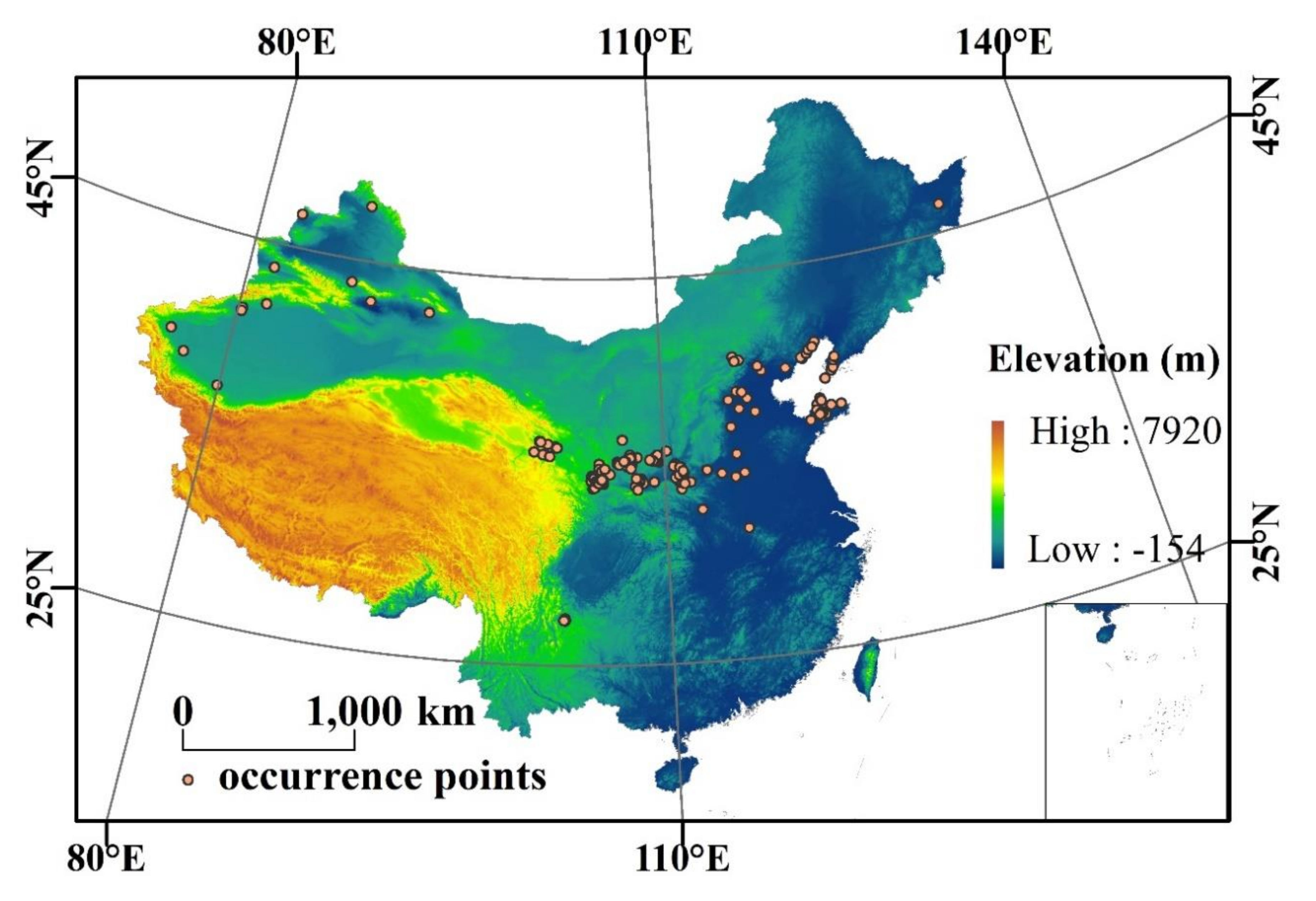
2.1. Species Occurrence Data and Environmental Variables

We gathered 93 occurrence points with GPS by our field survey, 12 occurrence points from 55 published studies from the Web of Science (WOS), and 168 occurrence points from 71 published reports from the China National Knowledge Infrastructure (CNKI). Removing widely marked points and duplicated sites, we gathered 211 available points. The points from published studies were positioned by GoogleEarth–pro if their GPS data were not recorded. To lessen the spatial autocorrelation effect, we finally obtained 158 rarefying data points (Figure 1 and Table A1 of Appendix A) with the criterion that there would be no more than one occurrence point in a grid cell (the distance between occurrence data > 5 km). We initially download 19 bioclimatic variables (bio1–bio19, 2.5 arc–min resolution, ~5 km) from WorldClim v2.1 [54] (https://www.worldclim.org/data/index.html), Digital Elevation Model (DEM, ~1 km) data and three soil texture data (~1 km) from the Data Center for Resource and Environment Sciences (RESDC, http://www.resdc.cn/), and one soil type data from the Harmonized World Soil Database (HWSD, http://www.fao.org/soils–portal/en) (Table A2 and Table A3). The data from WorldClim include current conditions (1970–2000) and future climate data (2030s: 2021–2040, 2050s: 2041–2060, 2070s: 2061–2080, and 2090s: 2081–2100). Variable selection is an effective way to deal with model overfitting [55,56]. We selected bio1 and bio12 as the climate factors based on the principal component analysis (PCA, Table A2) [37] of all bioclimatic variables (bio1–bio19), and then added bio6, bio11, and bio15 according to the incidence trends and physiology requirements [4,11] of V. mali.
In our study, the topographic data (including elevation, aspect, slope, and curvature) in the grid were calculated from DEM data by ArcGIS 10.2 (ESRI, Redlands, CA, USA). We also chose soil data, including soil texture (sand, silt, and clay) and soil type (FAOSoil: including sand%, silt%, clay%, pH2O, N%, CaCO3%, etc., of topsoil and subsoil), as the vital environmental data in our study. To avoid multicollinearity [36,57], we conducted a correlation analysis of selected bioclimatic, topographic, and soil data and removed those variables with a correlation coefficient greater than 0.8 (Table A3) [55]. We resampled all environmental data into 2.5 arc–min spatial resolution for the accuracy of the prediction and finally retained 11 environmental variables (Table 1) to model the current distribution of V. mali.

2.2. Climate Change Scenarios

The Shared Socioeconomic Pathways (SSPs) represent similar future radiative forcing pathways to the Representative Concentration Pathways (RCPs) in CMIP5: SSP1–26 (Low: 2.6 Wm−2), SSP2–45 (Medium: 4.5 Wm−2), SSP3–70 (High: 7.0 Wm−2), and SSP5–85 (High: 8.5 Wm−2) updated RCP2.6 (2.6 Wm−2, ~490 ppm CO2), RCP4.5 (4.5 Wm−2, ~650 ppm CO2), RCP6.0 (6.0 Wm−2, ~850 ppm CO2), and RCP8.5 (8.5 Wm−2, 1370 ppm CO2), respectively [58,59,60]. The emissions of future greenhouse gas increase from SSP1–26 to SSP5–85, and SSP2–45 is regarded as the stabilization scenario. During four forcing scenarios, only SSP1–26 achieved the goal of limit global temperature warming below 2 °C (SSP2–45: 2.6 °C, SSP3–70: 4.1 °C, and SSP5–85: 5.1 °C) at the end of the 21st century [40,59].
We chose the Beijing Climate Center Climate System Model (BCC–CSM2–MR) from nine global climate models (GCMs) as the bioclimatic variables in our study because it has been widely used in Asia [48,61], especially in China [36]. Considering the stability of the terrain [55], we assumed these relative variables would not change in this century. To provide plausible descriptions of future climate change, we used the same topography variables and soil data along with the similar bioclimatic variables of different periods to predict the future distribution of V. mali.

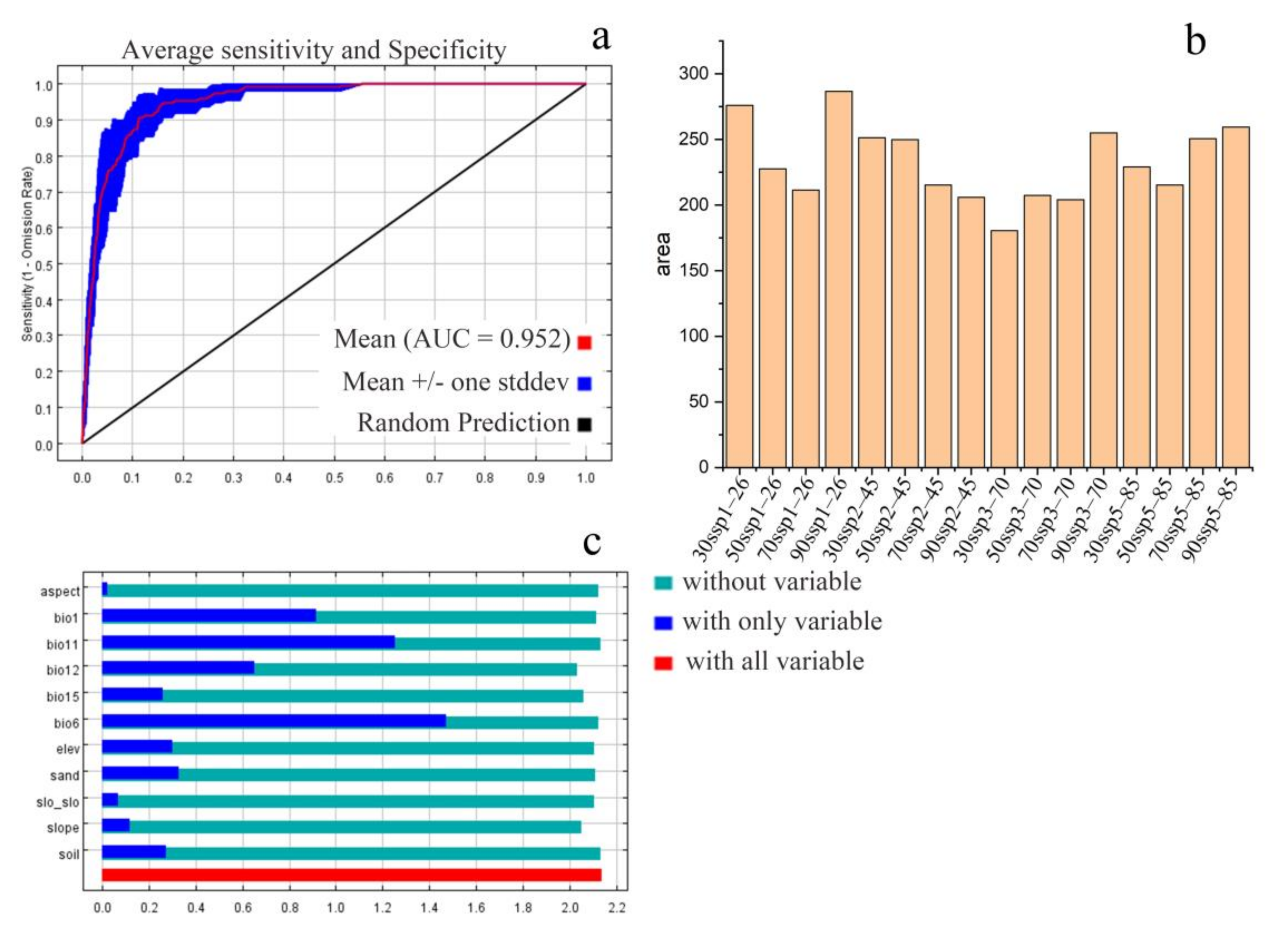
2.3. Species Distribution Model Evaluation

In this study, we used MaxEnt v3.4.1 [25], a machine learning algorithm program [62,63], to estimate the potential geographic distribution [47,64] and range shifts [36] of V. mali because of its wide use [24,27,65] and higher accuracy [66] compared with other SDMs [67] in predicting the distribution of species. Occurrence data (without absence data [15]) and environmental data [63,67,68] are required to run MaxEnt. The area under the receiver operating characteristic curve (AUC) is usually used to estimate the accuracy of prediction [69], and Jackknife test results were used to evaluate the relative importance of environmental variables [63]. In general, AUC values range from 0 to 1 [25]: ≤0.5 indicating bad prediction, >0.5 and ≤0.7 indicating fair prediction, >0.7 and ≤0.9 indicating good prediction, and >0.9 and ≤1 indicating excellent prediction [69,70].
In addition to the default settings, for sub–setting the present data, 25% of the occurrence data were used as test data and 75% as training data [45,71]. To predict the potential distribution of V. mali, 17 single models (i.e., one for the current distribution and 4 SSPs × 4 periods for the future) were built with parameters of 1000 maximum iterations and repeated 5 times for each process to reduce uncertainty [37]. Hence, we finally built a total of 165 model results (80 of them were replications for corresponding future predictions) in this step.
To delineate the presence and absence maps of V. mali, we averaged the probability values and created binary maps (suitable or not suitable) with “maximum test sensitivity plus specificity (Max sss, close to 0.05)” [29,35,72]. The presence/absence maps show the spatial distribution of V. mali. We then reclassified the distribution map into low suitable habitat (LSH), moderately suitable habitat (MSH), and highly suitable habitat (HSH) with break values of 0.2, 0.5, and 1.0, respectively.

2.4. Spatial and Statistical Analysis

The centroids, calculated by the averaging coordinates (latitude and longitude) of all suitable pixels in distribution maps [73], have been widely used in assessing the distributional changes in binary SDMs [45]. To illustrate the suitable habitat area changes of V. mali, (1) we measured the core range shifts by calculating centroids of suitability in different periods (present, 2030s, 2050s, 2070s and 2090s) and SSPs (SSP1–26, SSP2–45, SSP3–70, and SSP5–85), and demonstrated the direction of range shifts of different periods (i.e., 2030s–present, 2050s–2030s, 2070s–2050s, and 2090s–2070s) in different climate scenarios; (2) we calculated the area change ratio of suitable habitats with the equation Cr = (Aa − Ap)/Ap, where Cr represents the change ratio, and Aa and Ap represent the distribution area (1 × 10⁴ km2) of the following period and previous period [36]; (3) we distinguished the suitable area without suitability change from the unsuitable area and tested Moran’s index to measure the spatial autocorrelation of potential distribution with the help of ArcGIS 10.2. To fit the location of the study area, all geographic maps in our study were projected onto the Asia North Albers Equal Area Conic Projection.

3. Results

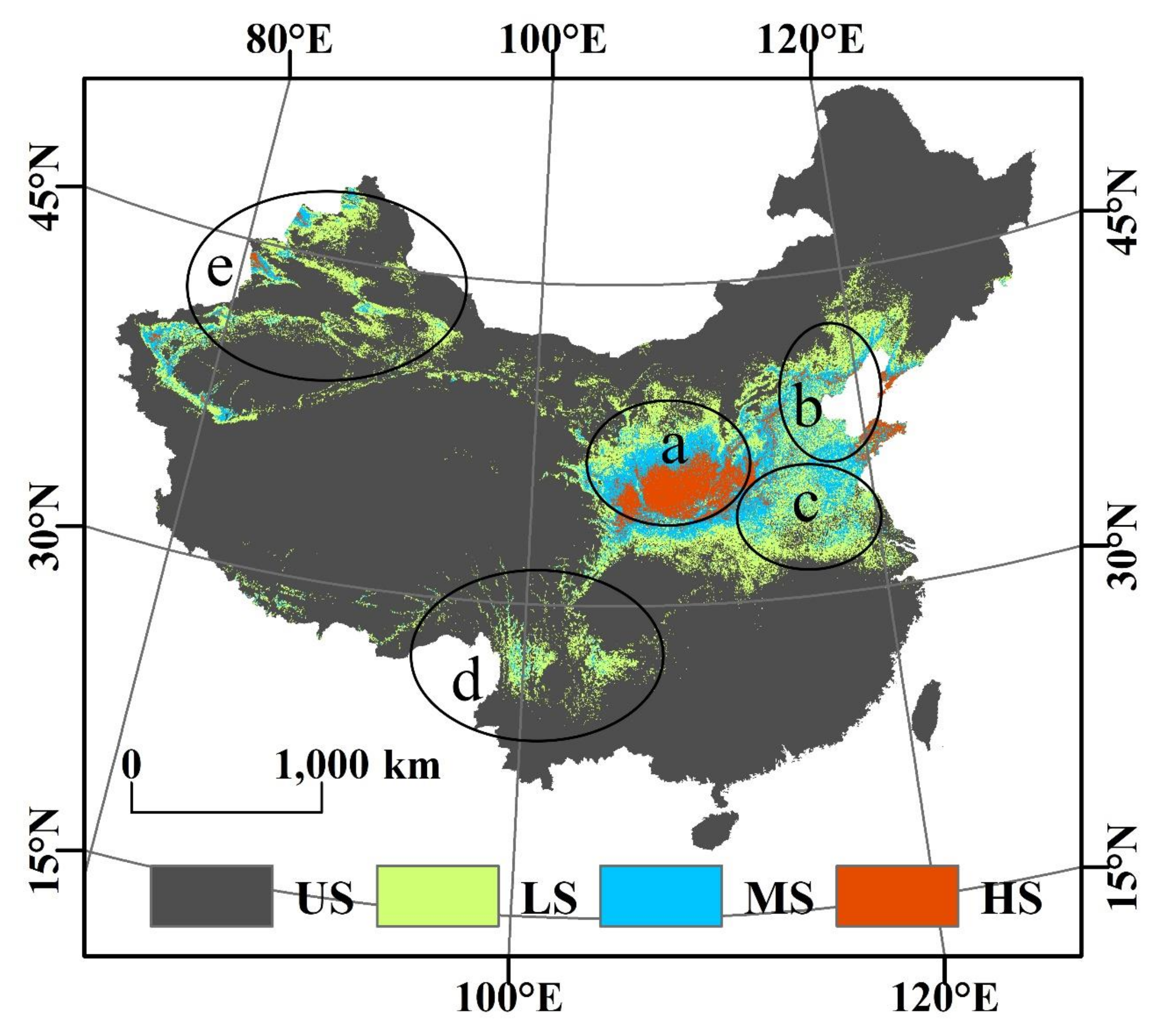
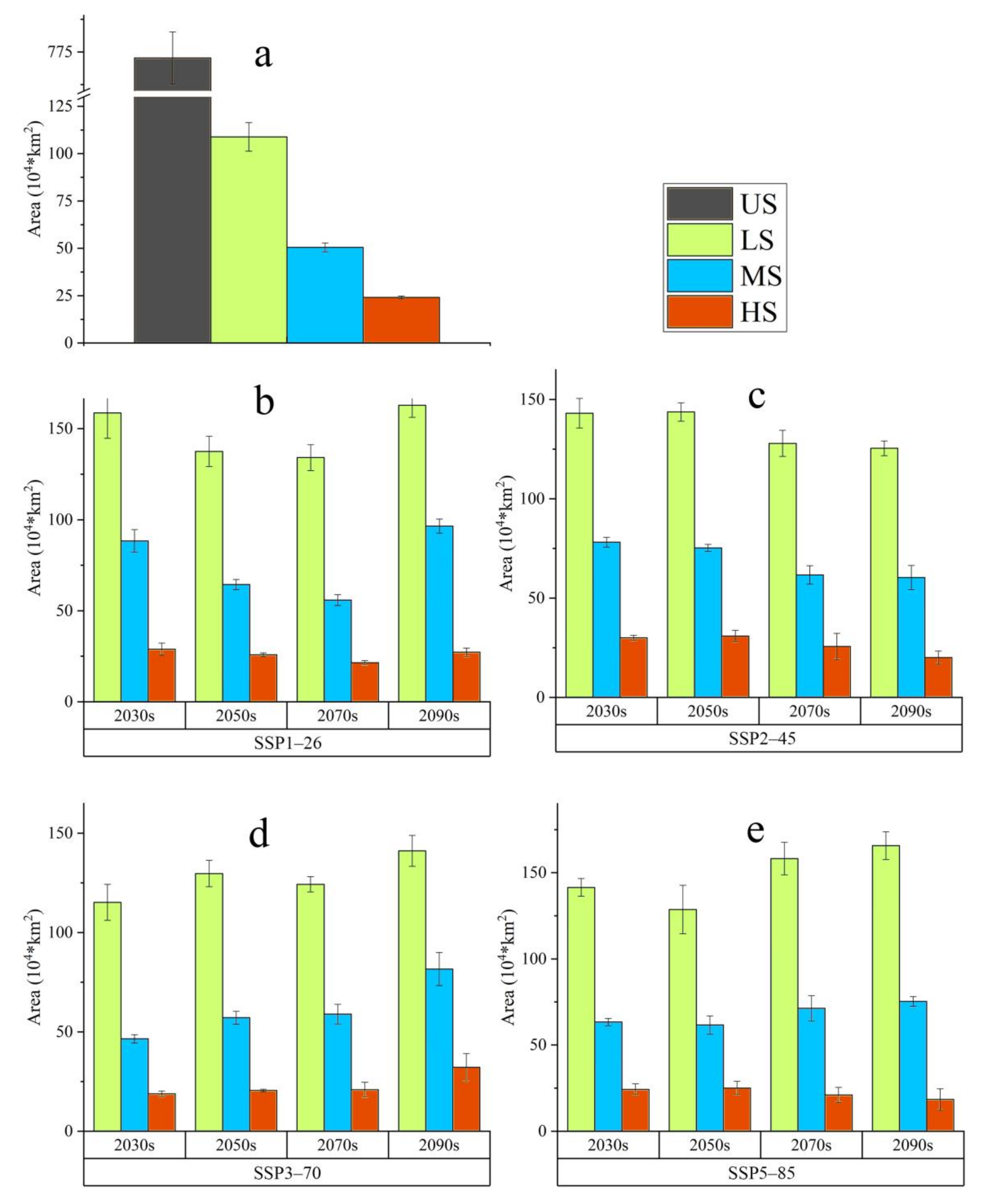
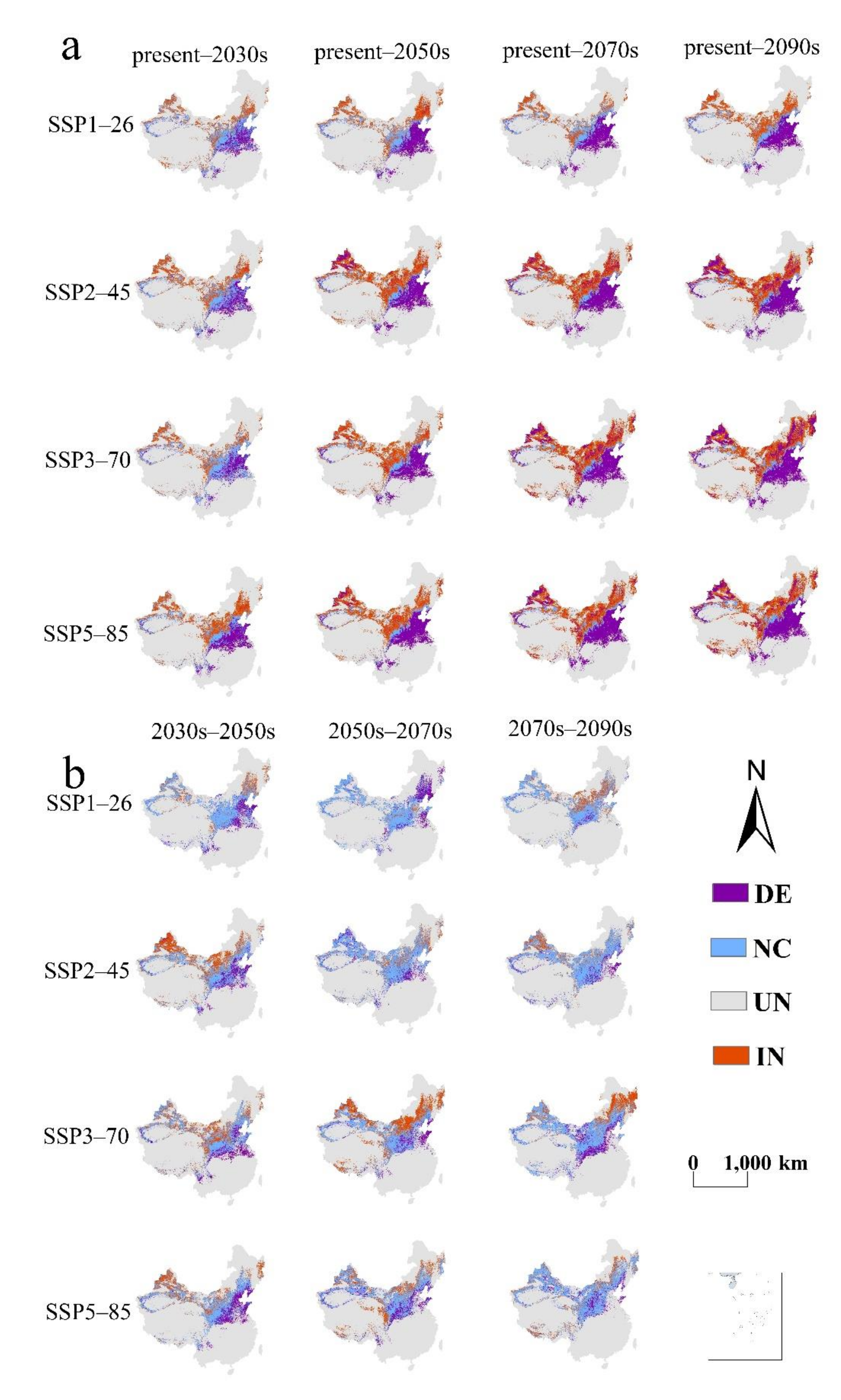
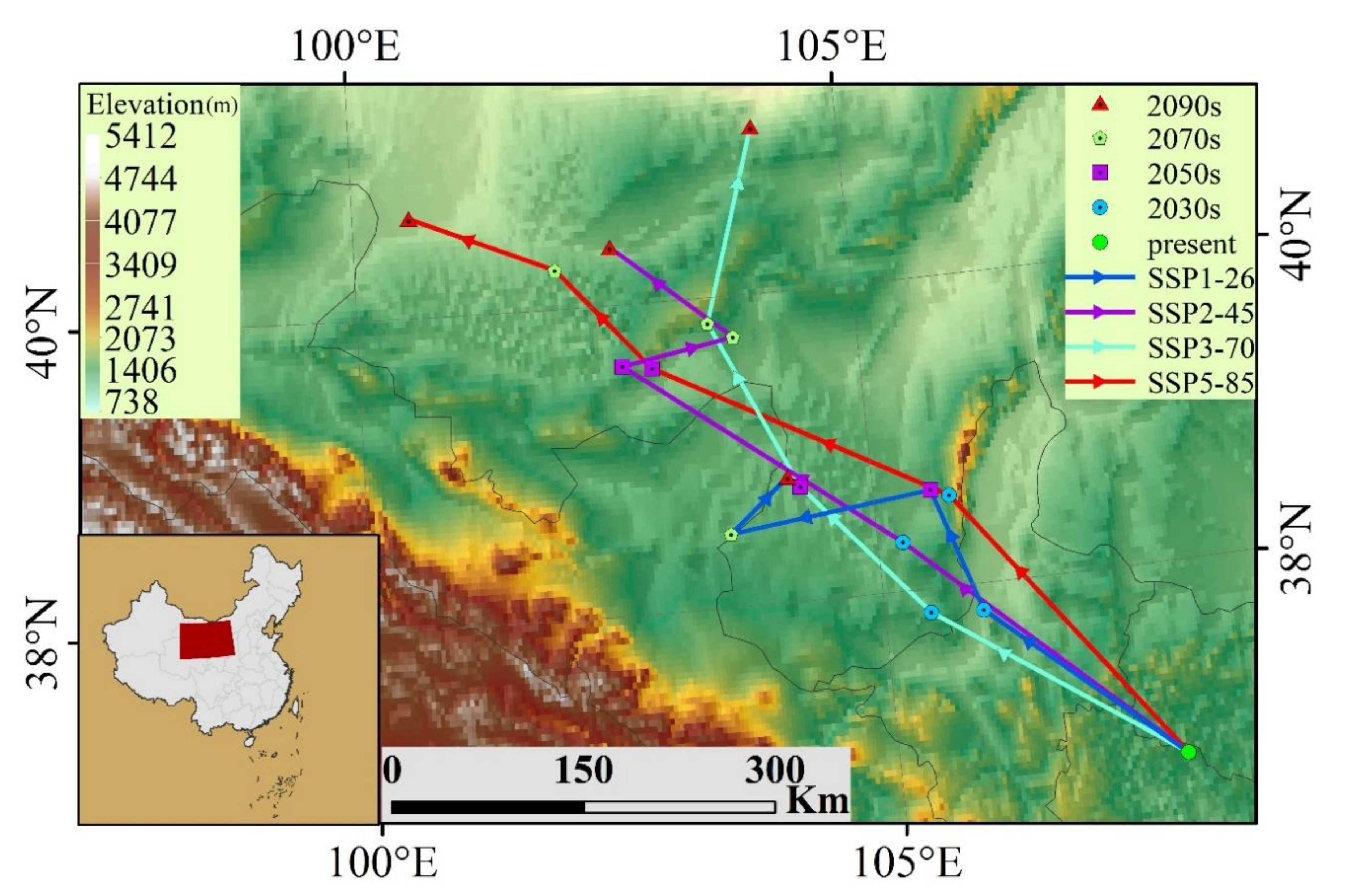
3.1. The Projected Distribution of V. mali

We obtained the distribution maps of V. mali under current and future climate scenarios (Figure 2 and Figure 3) and calculated the area of suitable habitats (Figure 4). In the current condition in China, with a 0.932 value of Moran’s index, the areas of unsuitable habitat (USH), low suitable habitat (LSH), moderately suitable habitat (MSH), and highly suitable habitat (HSH) were founded to be 772.70 × 10⁴ km2, 108.85 × 10⁴ km2, 50.52 × 10⁴ km2, and 24.09 × 10⁴ km2, respectively. The HSH area of SSP1–26 showed a U–shape from the 2030s to the 2090s, while those of SSP2–45 and SSP5–85 were an inverted U–shape (Figure 4). It is worth noting that, compared with the current distribution, almost all of the change ratios of LSH and MSH under four climate scenarios are positive in the 21st century, except for −7.92% of the present–2030s period under SSP3–70 (Figure 5a). Correspondingly, the change ratio of HSH was more complicated: the SSP3–70 climate scenario decreased with the average ratios of −21.83% (the 2030s), −14.77% (the 2050s), and −13.17% (the 2070s) and increased with 33.57% (the 2090s), while the SSP2–45 climate scenario increased with the average ratios of 24.76% (the 2030s), 28.32% (the 2050s), and 6.42% (the 2070s) and decreased with −16.78% (the 2090s) (Figure 5a and Figure 6a). Under the SSP1–26 scenario, the area of LSH, MSH, and HSH increased in the present–2030s period and the 2070s–2090s period, and decreased in the middle of the century (2030s–2050s and 2050s–2070s periods, Figure 5b and Figure 6b). The SSP3–70 scenario decreased the area of LSH, MSH, and HSH during the first 20 years (present–2030s) and increased the area from the 2030s to the 2090s except for the LSH of the 2050s–2070s period (Figure 5b).
In the current condition, the potential suitable area (LSH, MSH, and HSH) of V. mali is distributed in all five traditional apple–producing regions, which is more serious in the Bohai Bay area, the Old Yellow River Basin area, and the Loess Plateau area of Northwest China (Figure 2). With global warming, the suitability of potential distribution shows a major increase in the Xinjiang area, North China, and Northeast China and a decrease in the Bohai Bay area, the Old Yellow River Basin area, and east of the Loess Plateau area (Figure 6a).
The centroid of range shifts showed that V. mali, compared with the current centroid, would shift to the northwest direction (Figure 7). Under the SSP1–26, SSP2–45, SSP3–70 and SSP5–85 climate scenarios, the shift distance in the 2030s would be 199.18, 281.61, 238.10, and 269.55 km, respectively, while in the 2090s, the shift distance would be 388.97, 602.10, 572.55, and 758.44 km, respectively. From lower to higher SSP scenarios, the shift distance generally increased. The shift distance also increased under four climate scenarios from the present to the 2030s, the 2050s, the 2070s, and the 2090s.

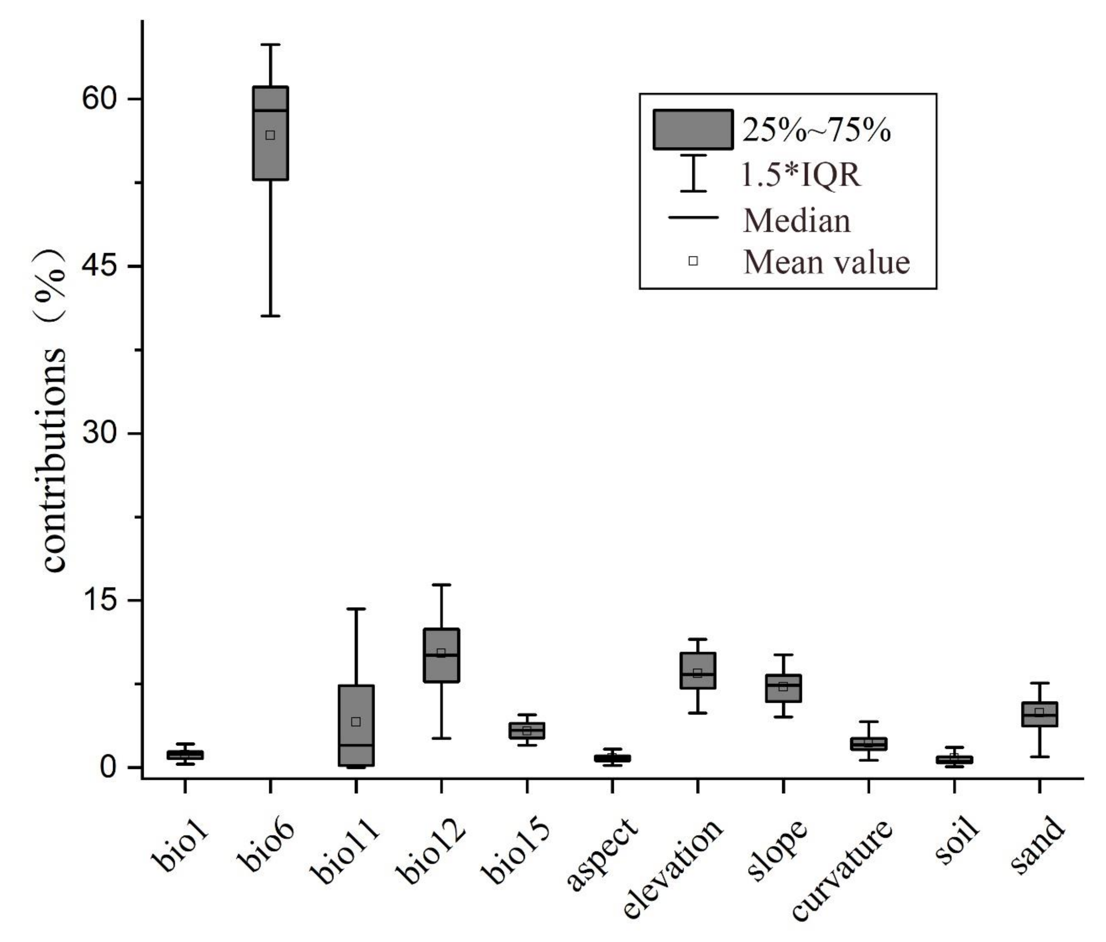
3.2. Contributions of Environmental Factors to the Distribution of V. mali

The MaxEnt model provided satisfactory projections with an average AUC value of 0.952 ± 0.009 (test, Figure A1a) and 0.965 ± 0.013 (training). Bioclimatic data, topographic data, and soil data all played a vital role in determining the distribution of V. mali. Among environmental variables, bioclimate variables contributed the most (a total of 75.54%), with bio6 and bio12 providing 56.73% and 10.27% of the contribution (Figure 8). Topographic variables ranked as the second most important factors with the average contribution of elevation and slope being 8.44% and 7.23%, respectively, while soil variables ranked third, with sand and soil contributing 4.88% and 0.87% to the MaxEnt model, respectively. In general, the cumulative value of the top five important variables (bio6, bio12, elevation, slope, and sand) was 87.54%. Interestingly, bio11 had a small contribution to MaxEnt, with an average contribution of only 4.11%, but it varied from 0.01% to 19.87%.

4. Discussion

4.1. Changes on the Suitable Habitat Area of V. mali

Our results successfully modeled the current distribution of V. mali and indicated that the suitable habitats will be optimistically affected by the anticipated climate, topographic, and soil factors in 2030s, 2050s, 2070s, and 2090s, except several specific periods of HSH may be negatively affected (Figure 5a). At the species scale, enough experiments have been performed to integrate the effects of climate change and other environmental variables on species range shifts [37]. Species that are sensitive to changes in temperature and precipitation will probably vary greatly in area and range shifts [43], and those with a narrow geographic range might be too vulnerable to extinction [36]. In our case, both SSP2–45 and SSP3–70 had reasonable expansion trends, and SSP1–26 and SSP5–85 had bigger expansion areas across the four climate scenarios. However, SSP3–70 might be the more plausible scenario for V. mali, considering both the increase area of HSH and MSH and their change trends. In addition, we observed a significant increase of suitability in Northwest, North, and Northeast China, both in terms of suitable classes and potential area (Figure 4 and Figure 6a). The corresponding increase of precipitation and temperature may be the internal dominate driver because the change of topographic factors, soil type, and soil texture factors are relatively slow in a short historical period [55]. With the continued increase of greenhouse gas emissions, a higher temperature increase is assumed from the lower emission scenario (SSP1–26) to the higher emission scenario (SSP5–85).
Previous studies have reported that species shifts to poleward in latitude and upward to higher elevation are the most frequent types of range shifts under the pressure of global warming [43,44,74]. In Southern Europe, studies of several forest pathogens showed the same shift trends due to climate change, resulting in the northward and upward spread [49]. However, the range shifts of V. mali showed an unexpectedly different direction, toward the northwest and lower elevations (Figure 7). Because the optimum temperature for V. mali to extend hyphae is approximately 20 °C [4], we speculate that the hydrothermal condition changes in suitable area mainly resulted in the unexpected shift type of the pathogen; affected by the southeast monsoon, the precipitation change caused by climate change may be the dominant factor. Global warming may lead to an average of 31% precipitation increase [40], which would have a significant impact on plant distribution patterns. In East Asia, although the southeast monsoon plays an important role relative to the open Northwest Pacific [75], the effects of the maritime climate are invariably weak in inland areas of Western China. In the arid and semiarid land of Western China, a slight increase in precipitation is enough to cause a dramatic change in the distribution of species. Considering the strong environment adaptability [11] of the conidial of V. mali, increasing precipitation may lead to a further expansion in the wild and in orchards than predicted. In addition, based on the range shift comparison of the present and future (Figure 6 and Figure 7), V. mali is expected to shift northwestward in all of the warming scenarios, which is similar to the direction of the southeast monsoon. To the best of our knowledge, the northwestward shift of V. mali is consistent with the shift of Rhododendrons in Southwest of China, but is the opposite in terms of vertical shift [36]. Because of high mountains located in both Southwest and Northwest China, we speculate the different response strategies of V. mali and Rhododendrons to temperature and precipitation may be the main reason for their opposite shifts in vertical direction. Precipitation (bio12) was found to play a more important role in the distribution of V. mali than temperature (bio1) in our study (Figure 8), and considering the complex topography of the suitable area, we believe that the downward range shift is also acceptable. Thus, the unexpected shift of species may be not so unexpected when the conditions of the local climate is taken into account [74].

4.2. The Role of Environmental Variables in Effecting the Distribution of V. mali and Corresponding Strategies for Preventing AVC

Any amount of caution is understandable when interpreting model–based results [45], for there are too many environmental variables and parameters that must be considered. The effects of environmental variables on the distribution of species may be disproportionate [76]. Our results indicate that climate factors have a stronger regulating effect on the distribution of V. mali than topographic and soil factors, and the temperature variables (bio1, bio6, and bio11) have a more significant effect than precipitation variables (bio12 and bio15; Figure 8 and Figure A1c). We assumed two possible reasons, and the first one focuses on the influence scale of environmental variable type. The predicted potential distribution of V. mali is spread over a wide area in Northern and Northwestern China. However, the change of topographic factors (i.e., aspect, elevation, slope, etc.) and soil factors (i.e., soil type and soil texture) generally affect the distribution of species in narrow spatial scale, while climate factors have been proved to be more influential on a broader scale [36,41]. Compared with climate factors, topographic and soil variables tend to affect the host of the pathogen. The second reason focuses on the infection strategy. Previous studies have confirmed that the primary infection paths of V. mali are pruning wounds (human factor) and rainwater (precipitation), and 80% of AVC is caused by pruning wounds, while wetness (precipitation) has not exhibited an essential effect [2,4]. The hyphal extension temperature of V. mali ranges from 5 to 35 °C (optimum at 20 °C), leading to the infection of the pathogen usually appearing in March, April, and May, declining from June and barely occurring in November and thereafter [4]. This is consistent with our results which show that temperature plays a more prominent role in affecting the distribution of V. mali than precipitation, and this explains why the minimum temperature of coldest month (bio6) contributed most to MaxEnt. Furthermore, at the wound, we speculate that water and temperature are probably complementary to V. mali infection, because in early spring, the alternations of ice melting and frost cracking often lead to worse AVC [77], especially of spur and bark wounds.
At the scale of the population level, the adaptive potential of the pathogen may reflect the effects of climate change [78], causing greater potential damage to trees [49]. Crabapple, the rootstocks of apple trees, has been identified along with apple seeds and seedlings as a potential inoculum source [79], which makes the control procedures of AVC more difficult. Therefore, to reduce the spread of V. mali, it is of vital importance to limit latent sources of infection: improving garden management methods to cultivate vigorous trees [3], coating new pruning wounds with protection film [4], and using special pruning tools for special gardens, as well as strengthening the management of diseased trees. In addition, the selection of biological agents [15], application of novel rapid assays [79], and nutritional dynamic monitoring of garden trees, especially leaf nutrient status of potassium content [3], are of great help to effectively decrease the occurrence and development of AVC, because suitable crop load management has been proved to increase the high–quality fruit percentage and plant resistance to AVC [80].

4.3. Limitations of SDMs in Projecting the Distribution of Species

Our study obtained the potential distribution maps of V. mali in several periods under four climate scenarios and successfully established an example for predicting the suitable habitats of a plant pathogen. However, the accuracy of our simulation is also affected by several limitations. Firstly, the accuracy of input data affects the accuracy of model results. Both the accuracy of species occurrence data and the selection of the current climate template increase the uncertainties of prediction [36]. Secondly, the selection of variables requires more rigorous methods. To avoid collinearity, we screened the environmental factors involved in model operation, but those factors that were filtered out by the screening process may contain potentially important information affecting the distribution of species. At the same time, the screened environmental variables have unstable performance in different simulations (i.e., the range of bio6 and bio11 in Figure 8). Thirdly, the model may limit the accuracy of prediction. The MaxEnt model assumes that species exist in habitats with similar environmental conditions, such as temperature and precipitation [67,81]. However, in the biological world, the presence of species is affected by more complex factors [71], which are often difficult to fully and accurately consider together. Unlike the simulated distributions, species may fail to disperse due to geographic barriers and real conditions of target regions [25,28]. In addition, some unquantifiable factors may affect the accuracy of simulation results due to their nonquantifiable characteristics. Especially, for some host–specific species (i.e., some plant pathogens), it is even difficult to distinguish the climate suitability between the species and its host [31]. We only considered abiotic factors [42] in our study, and biotic factors (i.e., human–caused land use change [36]) may also lead to changes of suitable habitat. Optimizing the algorithms in order to utilize more important information and to make the model more intelligent will further benefit the accuracy of simulation.

5. Conclusions

This study provided the potential distribution simulation of the pathogen of apple canker, V. mali, in the current and other periods of the 21st century under four CMIP6 climate scenarios: SSP1–26, SSP2–45, SSP3–70, and SSP5–85. In the current period, the predicted area of suitable habitat (LSH, MSH, and HSH) is 183.46 × 10⁴ km2. The suitable area will have different degrees of increase under all climate scenarios. In all scenarios, the range of potential suitable habitat shifted to the northwest, with the shift distance increasing from the 2030s to the 2090s, compared with the range of the present. The increase of suitability was found to be mainly in Xinjiang, and North and Northeast China, while the decrease was mainly in the Bohai Bay area, the Old Yellow River Basin area, and east of the Loess Plateau area. Till the end of this century, SSP1–26 has the biggest increase in total habitat area, and SSP3–70 was considered the optimum scenario for V. mali. We conclude that the dominant factors effecting the distribution of V. mali are temperature and corresponding precipitation, and temperature is considered to play a more important role.

Author Contributions

W.X. designed the study, finish model running, drew the figures and tables, and wrote the main body of the manuscript; J.J. supervision and analyzed the importance of factors; H.S. collected the occurrence data, provided methodology and analyzed the data; J.C. edited the draft, revised the manuscript, acquired the funding and revised the manuscript. All authors have read and agreed to the published version of the manuscript.

Funding

This research was supported by the Deployment Program of the Chinese Academy of Sciences (No. KJZD–EW–TZ–G10).

Acknowledgments

We acknowledge the groups of ArcGIS and MaxEnt for their contribution in making this simulation possible. WorldClim, RESDC, and FAO provided the raster data. We thank Hanqi Liu for his advice and assistance in data processing. Thanks to Runzhi Mao for his spiritual support. Especially, the authors would also like to thank the anonymous reviewers for their very important suggestions which have been particularly helpful in improving this paper.

Conflicts of Interest

The authors declare no conflict of interest.

Appendix A

Figure A1. The receiver operating characteristic curve (a), area of suitable habitats of Valsa mali in different climate scenarios (b), and the Jackknife test of environmental variables (c).
Forests 11 01126 g0a1
Table A1. The rarefying data points (158) of Valsa mali in China.
Occurrence PointLongitudeLatitudeOccurrence PointLongitudeLatitudeOccurrence PointLongitudeLatitude
Valsa mali105.245934.85065Valsa mali108.207934.33978Valsa mali105.812834.68276
Valsa mali105.206134.59958Valsa mali108.067334.2826Valsa mali105.991434.63819
Valsa mali105.359434.7649Valsa mali108.203734.10844Valsa mali105.901534.64976
Valsa mali107.214335.48161Valsa mali109.29434.48988Valsa mali111.112734.41605
Valsa mali106.9335.55836Valsa mali108.135734.69016Valsa mali110.947634.42388
Valsa mali107.603135.29842Valsa mali110.16936.05018Valsa mali110.940434.53704
Valsa mali105.76935.31032Valsa mali132.020746.44701Valsa mali110.844934.52789
Valsa mali105.72935.25686Valsa mali120.719536.97991Valsa mali111.660834.38018
Valsa mali105.774135.16865Valsa mali120.847637.33181Valsa mali111.249334.33246
Valsa mali105.718335.08535Valsa mali120.485537.63883Valsa mali112.744334.94146
Valsa mali105.723235.46861Valsa mali120.731237.92108Valsa mali114.779535.63555
Valsa mali105.721935.21247Valsa mali120.795137.79816Valsa mali113.706134.71211
Valsa mali106.913835.48206Valsa mali121.435237.50221Valsa mali115.111931.77896
Valsa mali107.043235.41133Valsa mali122.107437.50032Valsa mali114.572634.46878
Valsa mali105.476534.26437Valsa mali120.414537.34365Valsa mali115.188534.63789
Valsa mali105.324334.19708Valsa mali80.2580841.22645Valsa mali110.665135.34699
Valsa mali105.415834.24378Valsa mali80.3052941.32977Valsa mali112.294232.938
Valsa mali105.999534.44763Valsa mali80.2719441.15483Valsa mali110.737735.20919
Valsa mali105.887434.47668Valsa mali115.103440.60481Valsa mali110.599935.24551
Valsa mali105.858634.55483Valsa mali115.524640.41747Valsa mali110.680634.66079
Valsa mali105.787234.50759Valsa mali115.208640.37381Valsa mali110.931434.78846
Valsa mali107.977535.65879Valsa mali114.549938.42962Valsa mali111.041335.19894
Valsa mali107.853235.37529Valsa mali115.229637.92998Valsa mali111.245834.87806
Valsa mali107.896735.61616Valsa mali114.562737.04473Valsa mali111.200634.9765
Valsa mali108.230735.76626Valsa mali117.006539.75833Valsa mali119.917236.86932
Valsa mali106.428234.92928Valsa mali116.791540.01876Valsa mali120.99637.08069
Valsa mali105.835835.04372Valsa mali116.284537.69512Valsa mali120.789237.19028
Valsa mali107.805935.82949Valsa mali118.702939.73591Valsa mali120.701137.18603
Valsa mali107.828835.78574Valsa mali115.829838.42281Valsa mali120.578637.11801
Valsa mali107.753535.89863Valsa mali115.138438.83805Valsa mali81.8962441.79683
Valsa mali107.833735.65728Valsa mali115.505238.77561Valsa mali75.8671939.37309
Valsa mali107.596435.69838Valsa mali111.054934.05162Valsa mali77.1332938.36349
Valsa mali107.758335.74343Valsa mali110.89234.5089Valsa mali81.843143.72794
Valsa mali107.472435.55178Valsa mali111.096134.71984Valsa mali79.9255137.11503
Valsa mali107.356535.58652Valsa mali111.18934.77284Valsa mali82.9956646.75049
Valsa mali105.882835.09036Valsa mali102.333735.88342Valsa mali87.6083243.80811
Valsa mali106.106635.19679Valsa mali101.778836.60275Valsa mali88.1428247.84309
Valsa mali109.640435.50803Valsa mali102.83236.35028Valsa mali89.212442.96021
Valsa mali109.607835.58897Valsa mali102.951536.28235Valsa mali93.5218242.8085
Valsa mali109.59135.70494Valsa mali102.025735.94011Valsa mali103.64627.45558
Valsa mali109.440935.77218Valsa mali102.320736.47386Valsa mali103.591127.37106
Valsa mali109.568835.85828Valsa mali101.853636.58037Valsa mali103.644127.35729
Valsa mali108.452834.64583Valsa mali102.479135.84351Valsa mali121.304138.90109
Valsa mali108.602334.43616Valsa mali101.447536.05149Valsa mali121.804139.26661
Valsa mali107.269236.69266Valsa mali105.908934.53902Valsa mali121.963839.39049
Valsa mali109.257335.56844Valsa mali105.555834.56248Valsa mali122.06539.78451
Valsa mali109.059935.61743Valsa mali105.500934.5597Valsa mali122.158539.94054
Valsa mali107.796135.20038Valsa mali105.64434.60327Valsa mali119.949540.09864
Valsa mali108.365734.53922Valsa mali105.710434.47127Valsa mali119.856640.14749
Valsa mali120.738240.61335Valsa mali120.94940.85481Valsa mali120.292840.31371
Valsa mali120.440440.49809Valsa mali120.819540.72228
Table A2. Eigenvalues of 19 bioclimatic variables in principle component analysis.
VariablePercent of Eigenvalues (%)Accumulative of Eigenvalues (%)
bio181.9081.90
bio1217.6399.53
bio60.3799.91
bio160.0399.94
bio70.0399.97
bio180.0199.98
bio190.0199.99
bio170.0099.99
bio150.0099.99
bio140.0099.99
bio130.0099.99
bio110.0099.99
bio100.0099.99
bio90.0099.99
bio80.0099.99
bio50.0099.99
bio40.0099.99
bio30.0099.99
bio20.00100.00
Table A3. Correlation matrix of topographic and soil data.
SoilSlopAspectCurvatureSandSiltClay
soil1
slop−0.012081
aspect−0.001730.010111
curvature−0.07395−0.0869−0.074721
sand−0.009150.00656−0.005490.086971
silt−0.07583−0.007150.0032−0.09976−0.880741
clay0.08828−0.004930.00646−0.05828−0.840.567781

References

  1. Qu, Z.; Zhou, G. Possible Impact of Climate Change on the Quality of Apples from the Major Producing Areas of China. Atmosphere 2016, 7, 113. [Google Scholar] [CrossRef] [Green Version]
  2. Wang, L.; Zang, R.; Huang, L.L.; Xie, F.Q.; Gao, X.N. The investigation of apple tree Valsa canker in Guanzhong region of Shaanxi Province. J. Northwest Sci Tech Univ. Agric. For. (Nat. Sci. Ed.) 2005, 33, 98–100. [Google Scholar]
  3. Peng, H.X.; Wei, X.Y.; Xiao, Y.X.; Sun, Y.; Biggs, A.R.; Gleason, M.L.; Shang, S.P.; Zhu, M.Q.; Guo, Y.Z.; Sun, G.Y. Management of Valsa Canker on Apple with Adjustments to Potassium Nutrition. Plant Dis. 2016, 100, 884–889. [Google Scholar] [CrossRef] [Green Version]
  4. Chen, C.; Li, B.-H.; Dong, X.-L.; Wang, C.-X.; Lian, S.; Liang, W.-X. Effects of Temperature, Humidity, and Wound Age on Valsa mali Infection of Apple Shoot Pruning Wounds. Plant Dis. 2016, 100, 2394–2401. [Google Scholar] [CrossRef] [Green Version]
  5. Bessho, H.; Tsuchiya, S.; Soejima, J. Screening methode of apple–trees for resistance to Valsa canker. Euphytica 1994, 77, 15–18. [Google Scholar] [CrossRef]
  6. Yin, Z.; Ke, X.; Kang, Z.; Huang, L. Apple resistance responses against Valsa mali revealed by transcriptomics analyses. Physiol. Mol. Plant Pathol. 2016, 93, 85–92. [Google Scholar] [CrossRef]
  7. Wang, C.; Guan, X.; Wang, H.; Li, G.; Dong, X.; Wang, G.; Li, B. Agrobacterium tumefaciens–Mediated Transformation of Valsa mali: An Efficient Tool for Random Insertion Mutagenesis. Sci. World J. 2013. [Google Scholar] [CrossRef] [Green Version]
  8. Wang, X.; Zang, R.; Yin, Z.; Kang, Z.; Huang, L. Delimiting cryptic pathogen species causing apple Valsa canker with multilocus data. Ecol. Evol. 2014, 4, 1369–1380. [Google Scholar] [CrossRef] [PubMed]
  9. Nabi, S.U.; Raja, W.H.; Mir, J.I.; Sharma, O.C.; Singh, D.B.; Sheikh, M.A.; Yousuf, N.; Kamil, D. First Report Ofdiplodia Bulgarica a New Species Causing Canker Disease of Apple (Malus Domestica Borkh) in India. J. Plant Pathol. 2020, 102, 555–556. [Google Scholar] [CrossRef] [Green Version]
  10. Liu, X.; Li, X.; Bozorov, T.A.; Ma, R.; Ma, J.; Zhang, Y.; Yang, H.; Li, L.; Zhang, D. Characterization and Pathogenicity of Six Cytospora Strains Causing Stem Canker of Wild Apple in the Tianshan Forest, China. For. Pathol. 2020. [Google Scholar] [CrossRef]
  11. Wang, S.T.; Hu, T.L.; Wang, Y.A.; Luo, Y.; Michailides, T.J.; Cao, K.Q. New understanding on infection processes of Valsa canker of apple in China. Eur. J. Plant Pathol. 2016, 146, 531–540. [Google Scholar] [CrossRef]
  12. Chen, C.; Liu, F.; Xing, Z.; Zham, X.; Shi, X.; Guo, J.; Chen, Y. On the resistance of apple trees to the invasion by Valsa mali Miyabe et Yamada: Observations on the relationship between wound healing capacity of apple bark and the leave of resistance. Acta Phytopathol. Sin. 1982, 12, 49–55. [Google Scholar]
  13. Ke, X.W.; Huang, L.L.; Han, Q.M.; Gao, X.N.; Kang, Z.S. Histological and cytological investigations of the infection and colonization of apple bark by Valsa mali var. mali. Australas. Plant Pathol. 2013, 42, 85–93. [Google Scholar] [CrossRef]
  14. Yu, C.; Li, T.; Shi, X.; Saleem, M.; Li, B.; Liang, W.; Wang, C. Deletion of Endo–beta–1,4–Xylanase VmXyl1 Impacts the Virulence of Valsa mali in Apple Tree. Front. Plant Sci. 2018, 9. [Google Scholar] [CrossRef] [PubMed] [Green Version]
  15. Duan, S.; Du, Y.; Hou, X.; Yan, N.; Dong, W.; Mao, X.; Zhang, Z. Chemical Basis of the Fungicidal Activity of Tobacco Extracts against Valsa mali. Molecules 2016, 21, 1743. [Google Scholar] [CrossRef] [Green Version]
  16. Hu, Y.; Dai, Q.; Liu, Y.; Yang, Z.; Song, N.; Gao, X.; Voegele, R.T.; Kang, Z.; Huang, L. Agrobacterium tumefaciens–Mediated Transformation of the Causative Agent of Valsa canker of Apple Tree Valsa mali var. mali. Curr. Microbiol. 2014, 68, 769–776. [Google Scholar] [CrossRef]
  17. Ma, R.; Liu, Y.M.; Yin, Y.X.; Tian, C.M. A canker disease of apple caused by Cytospora parasitica recorded in China. For. Pathol. 2018, 48. [Google Scholar] [CrossRef]
  18. Liu, C.; Fan, D.; Li, Y.; Chen, Y.; Huang, L.; Yan, X. Transcriptome analysis of Valsa mali reveals its response mechanism to the biocontrol actinomycete Saccharothrix yanglingensis Hhs.015. BMC Microbiol. 2018, 18, 90. [Google Scholar] [CrossRef] [PubMed]
  19. Yin, Z.; Ke, X.; Li, Z.; Chen, J.; Gao, X.; Huang, L. Unconventional Recombination in the Mating Type Locus of Heterothallic Apple Canker Pathogen Valsa mali. G3–Genes Genomes Genet. 2017, 7, 1259–1265. [Google Scholar] [CrossRef] [Green Version]
  20. Wu, Y.; Xu, L.; Liu, J.; Yin, Z.; Gao, X.; Feng, H.; Huang, L. A mitogen–activated protein kinase gene (VmPmk1) regulates virulence and cell wall degrading enzyme expression in Valsa mall. Microb. Pathog. 2017, 111, 298–306. [Google Scholar] [CrossRef]
  21. Wang, N.N.; Yan, X.; Gao, X.N.; Niu, H.J.; Kang, Z.S.; Huang, L.L. Purification and characterization of a potential antifungal protein from Bacillus subtilis E1R–J against Valsa mali. World J. Microbiol. Biotechnol. 2016, 32, 63. [Google Scholar] [CrossRef]
  22. Nouri, M.T.; Lawrence, D.P.; Holland, L.A.; Doll, D.A.; Kallsen, C.E.; Culumber, C.M.; Trouillas, F.P. Identification and Pathogenicity of Fungal Species Associated with Canker Diseases of Pistachio in California. Plant Dis. 2019, 103, 2397–2411. [Google Scholar] [CrossRef] [PubMed]
  23. Kamiri, L.K.; Laemmlen, F.F. Epidemiology of cytospora canker caused in Colorado blue spruce by Valsa kunzei [Picea pungens]. Phytopathology 1981, 71, 941–947. [Google Scholar] [CrossRef]
  24. Abolmaali, S.M.-R.; Tarkesh, M.; Bashari, H. MaxEnt modeling for predicting suitable habitats and identifying the effects of climate change on a threatened species, Daphne mucronata, in central Iran. Ecol. Inform. 2018, 43, 116–123. [Google Scholar] [CrossRef]
  25. Phillips, S.J.; Anderson, R.P.; Schapire, R.E. Maximum entropy modeling of species geographic distributions. Ecol. Model. 2006, 190, 231–259. [Google Scholar] [CrossRef] [Green Version]
  26. Halvorsen, R.; Mazzoni, S.; Dirksen, J.W.; Næsset, E.; Gobakken, T.; Ohlson, M. How important are choice of model selection method and spatial autocorrelation of presence data for distribution modelling by MaxEnt? Ecol. Model. 2016, 328, 108–118. [Google Scholar] [CrossRef]
  27. Zhang, K.; Yao, L.; Meng, J.; Tao, J. Maxent modeling for predicting the potential geographical distribution of two peony species under climate change. Sci. Total Environ. 2018, 634, 1326–1334. [Google Scholar] [CrossRef]
  28. Guisan, A.; Zimmermann, N.E. Predictive habitat distribution models in ecology. Ecol. Model. 2000, 135, 147–186. [Google Scholar] [CrossRef]
  29. Liu, C.; White, M.; Newell, G. Selecting thresholds for the prediction of species occurrence with presence–only data. J. Biogeogr. 2013, 40, 778–789. [Google Scholar] [CrossRef]
  30. Narouei-Khandan, H.A.; Worner, S.P.; Viljanen, S.L.H.; van Bruggen, A.H.C.; Jones, E.E. Projecting the suitability of global and local habitats for myrtle rust (Austropuccinia psidii) using model consensus. Plant Pathol. 2020, 69, 17–27. [Google Scholar] [CrossRef]
  31. Narouei-Khandan, H.A. Ensemble Models to Assess the Risk of Exotic Plant Pathogens in a Changing Climate, in Lincoln; Lincoln University: Lincoln, New Zealand, 2014; pp. 220–221. [Google Scholar]
  32. Arteaga, V.L.; Lima, C.H.R. Analysis of CMIP 5 simulations of key climate indices associated with the South America monsoon system. Int. J. Climatol. 2020, 19. [Google Scholar] [CrossRef]
  33. Pascoe, C.; Lawrence, B.N.; Guilyardi, E.; Juckes, M.; Taylor, K.E. Documenting numerical experiments in support of the Coupled Model Intercomparison Project Phase 6 (CMIP6). Geosci. Model Dev. 2020, 13, 2149–2167. [Google Scholar] [CrossRef]
  34. Papes, M.; Gaubert, P. Modelling ecological niches from low numbers of occurrences: Assessment of the conservation status of poorly known viverrids (Mammalia, Carnivora) across two continents. Divers. Distrib. 2007, 13, 890–902. [Google Scholar] [CrossRef]
  35. Xu, X.; Zhang, H.; Yue, J.; Xie, T.; Xu, Y.; Tian, Y. Predicting Shifts in the Suitable Climatic Distribution of Walnut (Juglans regia L.) in China: Maximum Entropy Model Paves the Way to Forest Management. Forests 2018, 9, 103. [Google Scholar] [CrossRef] [Green Version]
  36. Yu, F.Y.; Wang, T.J.; Groen, T.A.; Skidmore, A.K.; Yang, X.F.; Ma, K.P.; Wu, Z.F. Climate and land use changes will degrade the distribution of Rhododendrons in China. Sci. Total Environ. 2019, 659, 515–528. [Google Scholar] [CrossRef]
  37. Guo, Y.L.; Li, X.; Zhao, Z.F.; Nawaz, Z. Predicting the impacts of climate change, soils and vegetation types on the geographic distribution of Polyporus umbellatus in China. Sci. Total Environ. 2019, 648, 1–11. [Google Scholar] [CrossRef] [PubMed]
  38. Lv, X.; Zhou, G. Climatic Suitability of the Geographic Distribution of Stipa breviflora in Chinese Temperate Grassland under Climate Change. Sustainability 2018, 10, 3767. [Google Scholar] [CrossRef] [Green Version]
  39. Root, T.L.; Price, J.T.; Hall, K.R.; Schneider, S.H.; Rosenzweig, C.; Pounds, J.A. Fingerprints of global warming on wild animals and plants. Nature 2003, 421, 57–60. [Google Scholar] [CrossRef]
  40. Bracegirdle, T.J.; Krinner, G.; Tonelli, M.; Haumann, F.A.; Naughten, K.A.; Rackow, T.; Roach, L.A.; Wainer, I. Twenty first century changes in Antarctic and Southern Ocean surface climate in CMIP6. Atmos. Sci. Lett. 2020, 14, e984. [Google Scholar] [CrossRef]
  41. Overpeck, J.T.; Rind, D.; Goldberg, R.J.N. Climate–induced changes in forest disturbance and vegetation. Nature 1990, 343, 51–53. [Google Scholar] [CrossRef]
  42. Cornelissen, B.; Neumann, P.; Schweiger, O. Global warming promotes biological invasion of a honey bee pest. Glob. Chang. Biol. 2019, 25, 3642–3655. [Google Scholar] [CrossRef] [PubMed] [Green Version]
  43. Chen, I.C.; Hill, J.K.; Ohlemuller, R.; Roy, D.B.; Thomas, C.D. Rapid Range Shifts of Species Associated with High Levels of Climate Warming. Science 2011, 333, 1024–1026. [Google Scholar] [CrossRef] [PubMed]
  44. Lenoir, J.; Gegout, J.C.; Marquet, P.A.; de Ruffray, P.; Brisse, H. A Significant Upward Shift in Plant Species Optimum Elevation During the 20th Century. Science 2008, 320, 1768–1771. [Google Scholar] [CrossRef] [PubMed]
  45. Wang, S.; Xu, X.; Shrestha, N.; Zimmermann, N.E.; Wang, Z. Response of spatial vegetation distribution in China to climate changes since the Last Glacial Maximum (LGM). PLoS ONE 2017, 12, e0175742. [Google Scholar] [CrossRef] [Green Version]
  46. Perry, C.T.; Alvarez-Filip, L. Changing geo–ecological functions of coral reefs in the Anthropocene. Funct. Ecol. 2019, 33, 976–988. [Google Scholar] [CrossRef] [Green Version]
  47. Ma, B.; Sun, J. Predicting the distribution of Stipa purpurea across the Tibetan Plateau via the MaxEnt model. BMC Ecol. 2018, 18, 10. [Google Scholar] [CrossRef] [Green Version]
  48. Rana, S.K.; Rana, H.K.; Ghimire, S.K.; Shrestha, K.K.; Ranjitkar, S. Predicting the impact of climate change on the distribution of two threatened Himalayan medicinal plants of Liliaceae in Nepal. J. Mt. Sci. 2017, 14, 558–570. [Google Scholar] [CrossRef]
  49. Porta, N.L.; Capretti, P.; Thomsen, I.M.; Kasanen, R.; Hietala, A.M.; Weissenberg, K.V. Forest pathogens with higher damage potential due to climate change in Europe. Can. J. Plant Pathol. 2008, 30, 177–195. [Google Scholar] [CrossRef]
  50. Zhong, L.; Ma, Y.M.; Salama, M.S.; Su, Z.B. Assessment of vegetation dynamics and their response to variations in precipitation and temperature in the Tibetan Plateau. Clim. Chang. 2010, 103, 519–535. [Google Scholar] [CrossRef]
  51. Na, L.; Wang, G.; Yan, Y.; Gao, Y.; Liu, G. Plant production, and carbon and nitrogen source pools, are strongly intensified by experimental warming in alpine ecosystems in the Qinghai–Tibet Plateau. Soil Biol. Biochem. 2011, 43, 942–953. [Google Scholar] [CrossRef]
  52. Guo, L.; Dai, J.H.; Wang, M.C.; Xu, J.C.; Luedeling, E. Responses of spring phenology in temperate zone trees to climate warming: A case study of apricot flowering in China. Agric. For. Meteorol. 2015, 201, 1–7. [Google Scholar] [CrossRef] [Green Version]
  53. Liu, C.; Chen, L.; Tang, W.; Peng, S.; Li, M.; Deng, N.; Chen, Y. Predicting Potential Distribution and Evaluating Suitable Soil Condition of Oil Tea Camellia in China. Forests 2018, 9, 487. [Google Scholar] [CrossRef] [Green Version]
  54. Fick, S.E.; Hijmans, R.J. WorldClim 2: New 1–km spatial resolution climate surfaces for global land areas. Int. J. Climatol. 2017, 37, 4302–4315. [Google Scholar] [CrossRef]
  55. Zhang, Q.; Wei, H.; Zhao, Z.; Liu, J.; Ran, Q.; Yu, J.; Gu, W. Optimization of the Fuzzy Matter Element Method for Predicting Species Suitability Distribution Based on Environmental Data. Sustainability 2018, 10, 3444. [Google Scholar] [CrossRef] [Green Version]
  56. Vaughan, I.P.; Ormerod, S.J. The Continuing Challenges of Testing Species Distribution Models. J. Appl. Ecol. 2005, 42, 720–730. [Google Scholar] [CrossRef]
  57. Touré, D.; Ge, J. The Response of Plant Species Diversity to the Interrelationships between Soil and Environmental Factors in the Limestone Forests of Southwest China. J. Environ. Earth Sci. 2014, 4, 105–122. [Google Scholar]
  58. Riahi, K.; van Vuuren, D.P.; Kriegler, E.; Edmonds, J.; O’Neill, B.C.; Fujimori, S.; Bauer, N.; Calvin, K.; Dellink, R.; Fricko, O.; et al. The Shared Socioeconomic Pathways and their energy, land use, and greenhouse gas emissions implications: An overview. Glob. Environ. Chang. Hum. Policy Dimens. 2017, 42, 153–168. [Google Scholar] [CrossRef] [Green Version]
  59. O’Neill, B.C.; Tebaldi, C.; van Vuuren, D.P.; Eyring, V.; Friedlingstein, P.; Hurtt, G.; Knutti, R.; Kriegler, E.; Lamarque, J.F.; Lowe, J.; et al. The Scenario Model Intercomparison Project (ScenarioMIP) for CMIP6. Geosci. Model Dev. 2016, 9, 3461–3482. [Google Scholar] [CrossRef] [Green Version]
  60. Vuuren, D.P.V.; Edmonds, J.; Kainuma, M.; Riahi, K.; Thomson, A.; Hibbard, K.; Hurtt, G.C.; Kram, T.; Krey, V.; Lamarque, J.F. The representative concentration pathways: An overview. Clim. Chang. 2011, 109, 5–31. [Google Scholar] [CrossRef]
  61. Xin, X.G.; Zhang, L.; Zhang, J.; Wu, T.W.; Fang, Y.J. Climate Change Projections over East Asia with BCC_CSM1.1 Climate Model under RCP Scenarios. J. Meteorol. Soc. Jpn. 2013, 91, 413–429. [Google Scholar] [CrossRef] [Green Version]
  62. Dudik, M. Maximum Entropy Density Estimation and Modeling Geographic Distributions of Species; Princeton University: Princeton, NJ, USA, 2007. [Google Scholar]
  63. Elith, J.; Phillips, S.J.; Hastie, T.; Dudik, M.; Chee, Y.E.; Yates, C.J. A statistical explanation of MaxEnt for Ecologists. Divers. Distrib. 2011, 17, 43–57. [Google Scholar] [CrossRef]
  64. Khanum, R.; Mumtaz, A.S.; Kumar, S. Predicting impacts of climate change on medicinal asclepiads of Pakistan using Maxent modeling. Acta Oecologica Int. J. Ecol. 2013, 49, 23–31. [Google Scholar] [CrossRef]
  65. Qin, A.; Liu, B.; Guo, Q.; Bussmann, R.W.; Ma, F.; Jian, Z.; Xu, G.; Pei, S. Maxent modeling for predicting impacts of climate change on the potential distribution of Thuja sutchuenensis Franch., an extremely endangered conifer from southwestern China. Glob. Ecol. Conserv. 2017, 10, 139–146. [Google Scholar] [CrossRef]
  66. Garcia, K.; Lasco, R.; Ines, A.; Lyon, B.; Pulhin, F. Predicting geographic distribution and habitat suitability due to climate change of selected threatened forest tree species in the. Philippines. Appl. Geogr. 2013, 44, 12–22. [Google Scholar] [CrossRef]
  67. Guisan, A.; Graham, C.H.; Elith, J.; Huettmann, F.; Distri, N.S. Sensitivity of predictive species distribution models to change in grain size. Divers. Distrib. 2007, 13, 332–340. [Google Scholar] [CrossRef]
  68. Lv, W.; Li, Z.; Wu, X.; Ni, W.; Qv, W. Maximum Entropy Niche–Based Modeling (Maxent) of Potential Geographical Distributions of Lobesia Botrana (Lepidoptera: Tortricidae) in China; Computer and Computing Technologies in Agriculture; Springer: Berlin/Heidelberg, Germany, 2011; pp. 239–246. [Google Scholar]
  69. Hu, X.; Wu, F.; Guo, W.; Liu, N. Identification of Potential Cultivation Region fie Santalum album in China by the MaxEnt Ecologic Niche Model. Sci. Silvae Sin. 2014, 50, 27–33. [Google Scholar]
  70. Hanley, J.A.; McNeil, B.J. The meaning and use of the area under a receiver operating characteristic (ROC) curve. Radiology 1982, 143, 29–36. [Google Scholar] [CrossRef] [Green Version]
  71. Phillips, S.J.; Dudik, M. Modeling of species distributions with Maxent: New extensions and a comprehensive evaluation. Ecography 2008, 31, 161–175. [Google Scholar] [CrossRef]
  72. Liu, C.; Newell, G.; White, M. On the selection of thresholds for predicting species occurrence with presence–only data. Ecol. Evol. 2016, 6, 337–348. [Google Scholar] [CrossRef] [Green Version]
  73. Brown, J.L. SDMtoolbox: A python–based GIS toolkit for landscape genetic, biogeographic and species distribution model analyses. Methods Ecol. Evol. 2014, 5, 694–700. [Google Scholar] [CrossRef]
  74. Lenoir, J.; Svenning, J.C. Climate–related range shifts—A global multidimensional synthesis and new research directions. Ecography 2015, 38, 15–28. [Google Scholar] [CrossRef]
  75. Liu, S.H.; Li, J.G.; Sun, L.; Wang, G.H.; Tang, D.L.; Huang, P.; Yan, H.; Gao, S.; Liu, C.; Gao, Z.Q.; et al. Basin–wide responses of the South China Sea environment to Super Ty–phoon Mangkhut (2018). Sci. Total Environ. 2020, 731, 15. [Google Scholar] [CrossRef] [PubMed]
  76. Zhang, J.; Nielsen, S.E.; Chen, Y.H.; Georges, D.; Qin, Y.C.; Wang, S.S.; Svenning, J.C.; Thuiller, W. Extinction risk of North American seed plants elevated by climate and land–use change. J. Appl. Ecol. 2017, 54, 303–312. [Google Scholar] [CrossRef]
  77. Li, Z.; Liu, G.; Zhang, X. Review of reaearches on the Valsa canker of apple trees. North Fruits 2013, 4, 1–3. [Google Scholar]
  78. Garrett, K.A.; Dendy, S.P.; Frank, E.E.; Rouse, M.N.; Travers, S.E. Climate change effects on plant disease: Genomes to ecosystems. Annu. Rev. Phytopathol. 2006, 44, 489–509. [Google Scholar] [CrossRef] [Green Version]
  79. Xiang-Long, M.; Xing-Hua, Q.; Ze-Yuan, H.; Yong-Bin, G.; Ya-Nan, W.; Tong-le, H.; Li-Ming, W.; Ke-Qiang, C.; Shu-Tong, W. Latent Infection of Valsa mali in the Seeds, Seedlings and Twigs of Crabapple and Apple Trees is a Potential Inoculum Source of Valsa Canker. Sci. Rep. 2019, 9, 1–10. [Google Scholar] [CrossRef] [Green Version]
  80. Suo, G.-D.; Xie, Y.-S.; Zhang, Y.; Cai, M.-Y.; Wang, X.-S.; Chuai, J.-F. Crop load management (CLM) for sustainable apple production in China. Sci. Hortic. 2016, 211, 213–219. [Google Scholar] [CrossRef]
  81. Guisan, A.; Thuiller, W. Predicting species distribution: Offering more than simple habitat models. Ecol. Lett. 2005, 8, 993–1009. [Google Scholar] [CrossRef]
Figure 1. The occurrence data (158 points) of Valsa mali in China.
Forests 11 01126 g001
Figure 2. Potential distribution map of Valsa mali in the current climate environment. The US, LS, MS, and HS represent the suitability of unsuitable, low suitable, moderately suitable, and highly suitable, respectively. Five ellipses represent the major apple–producing area of China: (a) the Loess Plateau area, (b) the Bohai Bay area, (c) the Old Yellow River Basin area, (d) the Cold Highland area of Southwest China, and (e) the Xinjiang area.
Forests 11 01126 g002
Figure 3. Distribution maps of Valsa mali in different climate scenarios and periods (2030s, 2050s, 2070s, and 2090s) of the 21st century. The Shared Socioeconomic Pathways (SSPs) 1–26, SSP2–45, SSP3–70, and SSP5–85 represent four climate scenarios. The US, LS, MS, and HS represent the suitability of unsuitable, low suitable, moderately suitable, and highly suitable, respectively.
Forests 11 01126 g003
Figure 4. Suitable habitat area of the present (e) and future (2030s, 2050s, 2070s, and 2090s) under four climate scenarios: (a) SSP1–26, (b) SSP2–45, (c) SSP3–70, (d) SSP5–85. The US, LS, MS, and HS represent the suitability of unsuitable, low suitable, moderately suitable, and highly suitable, respectively. The error bars represent the standard deviation of area.
Forests 11 01126 g004
Figure 5. Habitat area change ratio of future–present (a) and 20–year equal intervals (b). The US LS, MS, and HS represent the suitability of unsuitable, low suitable, moderately suitable, and highly suitable, respectively. The formulas with “–” represent the intervals of change ratio (i.e., present–2030s represents the period from the present to the 2030s). The Shared Socioeconomic Pathways (SSPs) 1–26, SSP2–45, SSP3–70, and SSP5–85 represent four climate scenarios.
Forests 11 01126 g005
Figure 6. Change in suitability of Valsa mali under four future climate scenarios (the Shared Socioeconomic Pathways (SSP) 1–26, SSP2–45, SSP3–70, and SSP5–85): future–present intervals (a) and 20–year equal intervals (b). The formulas with “–” represent the intervals which are used to calculate the suitability changes (i.e., 2030s–2050s represent the period from the 2030s to the 2050s). The DE, NC, UN, and IN represent decrease, no–change, unsuitable, and increase in suitability of V. mali.
Forests 11 01126 g006
Figure 7. Suitable area shifts (based on the centroid of suitable distribution map) of Valsa mali in four climate scenarios (the Shared Socioeconomic Pathways (SSP) 1–26, SSP2–45, SSP3–70, and SSP5–85).
Forests 11 01126 g007
Figure 8. Contributions of environmental factors in the MaxEnt model. The IQR represents inter quartile range.
Forests 11 01126 g008
Table 1. Environmental variables used in predicting the potential distribution of Valsa mali.
CategoryVariableDescriptionUnit
Bioclimatebio1Annual Mean Temperature°C
bio6Min Temperature of Coldest Month°C
bio11Mean Temperature of Coldest Quarter°C
bio12Annual Precipitationmm
bio15Precipitation Seasonality
TopographicaspectAspect
curvatureCurvature
elevationElevationm
slopeSlope°
SoilsandTexture of Soil
soilType of Soil
Publisher’s Note: MDPI stays neutral with regard to jurisdictional claims in published maps and institutional affiliations.

