Pollen Morphology and Variability of Abies alba Mill. Genotypes from South-Western Poland

 , ,
, ,  , ,
, ,
Abstract
:
1. Introduction
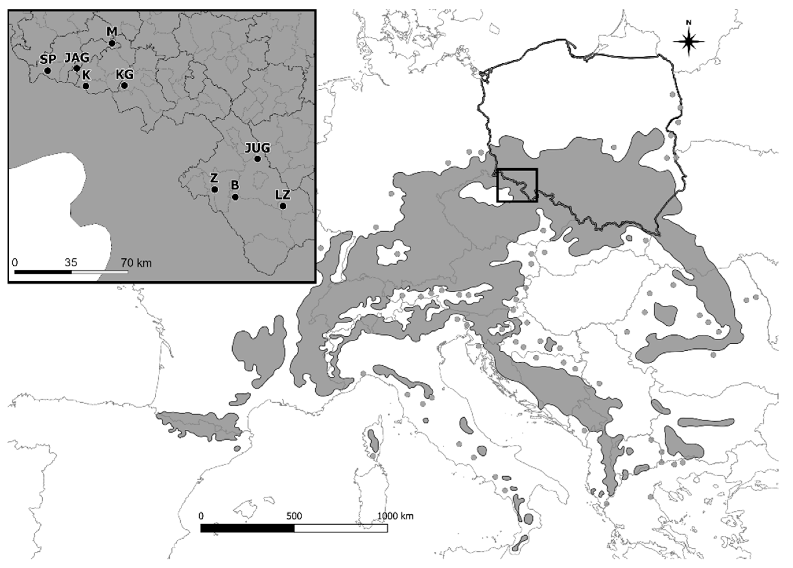
2. Material and Methods
2.1. Sampling and Genotyping
2.2. Palynological Analysis
2.3. Statistical Analysis
2.3.1. Genetic Analysis
2.3.2. Palynological Analysis
3. Results
3.1. Genetic Variability
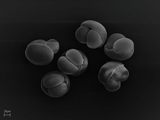
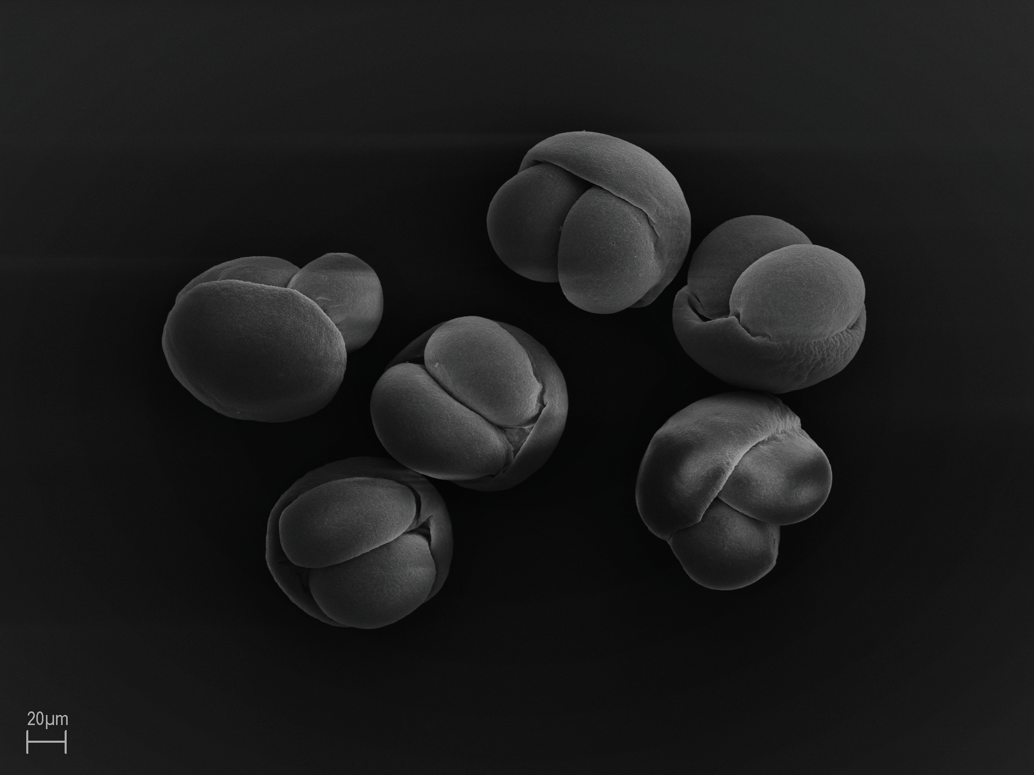
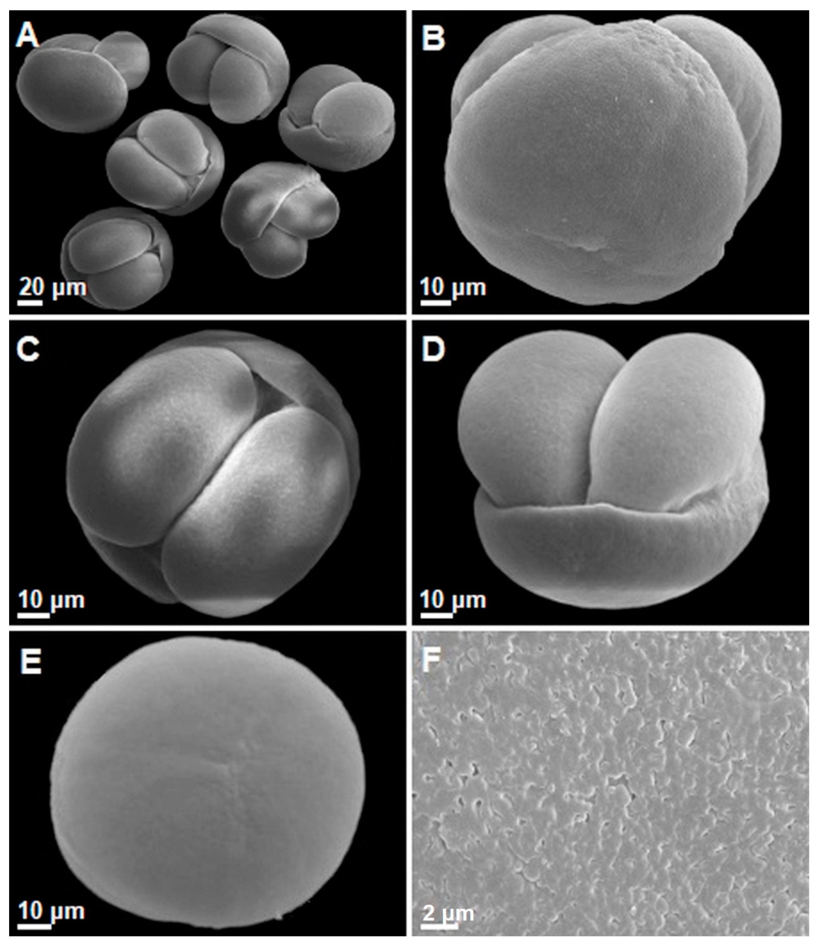
3.2. General Morphological Description of Pollen
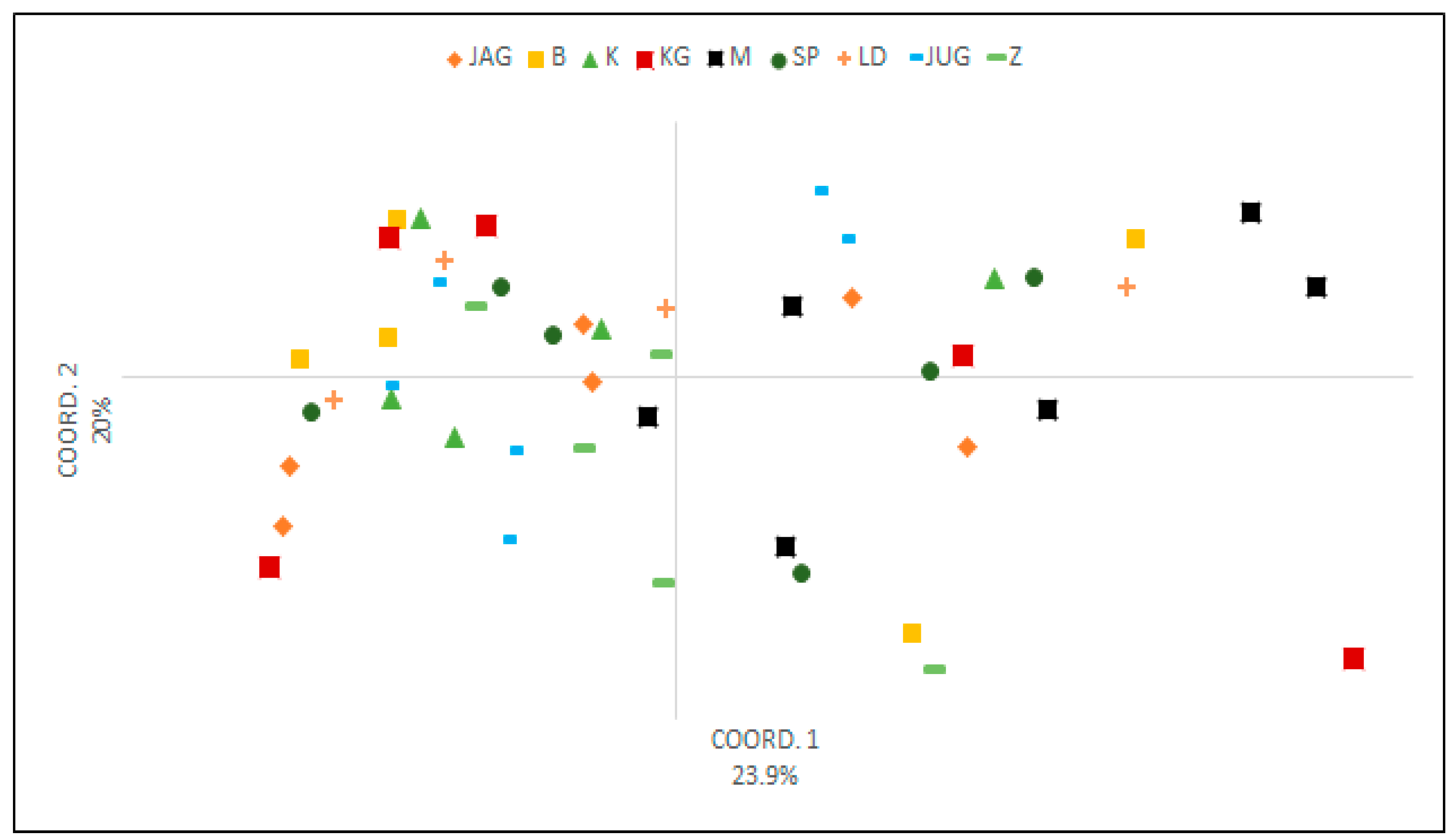
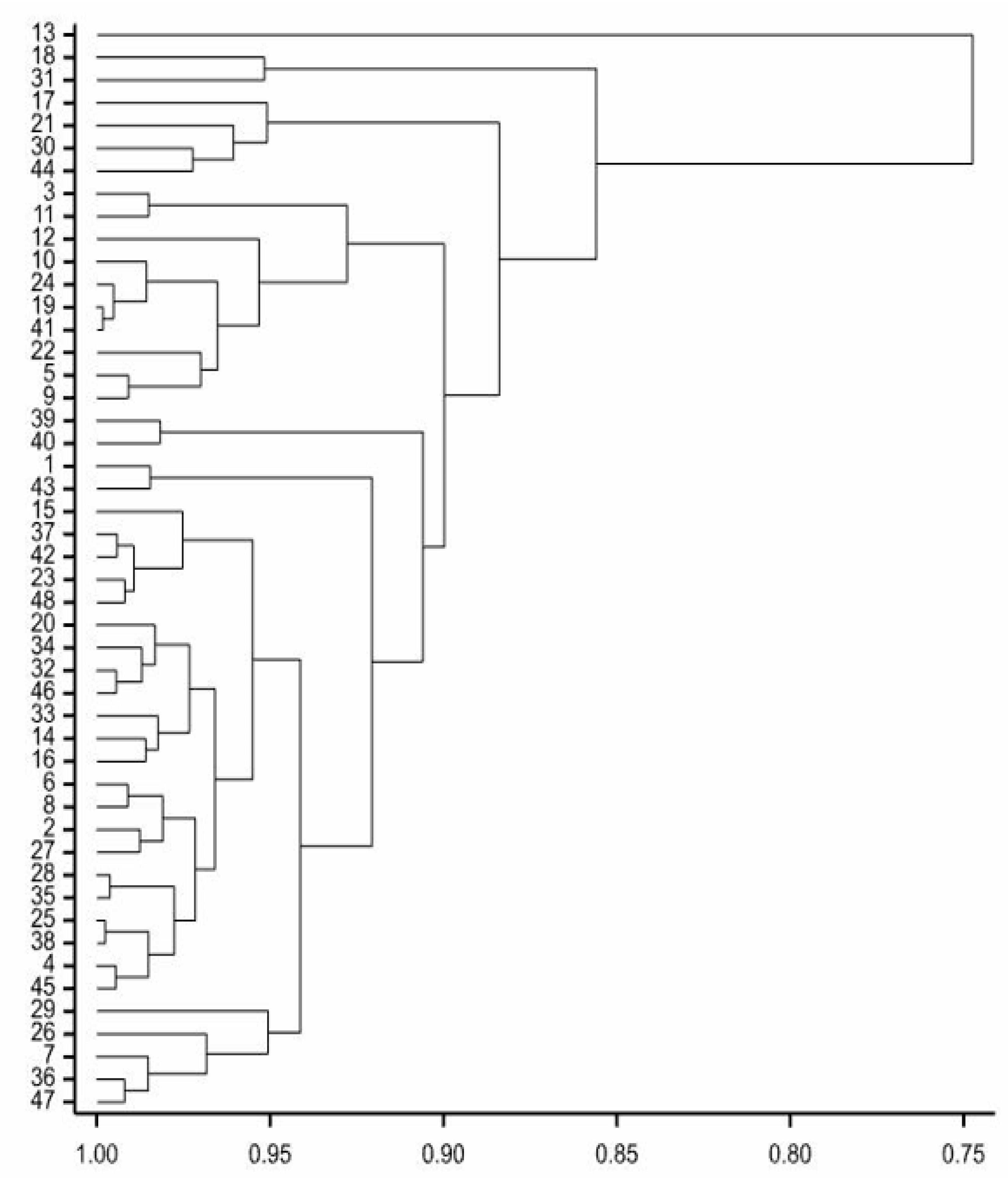
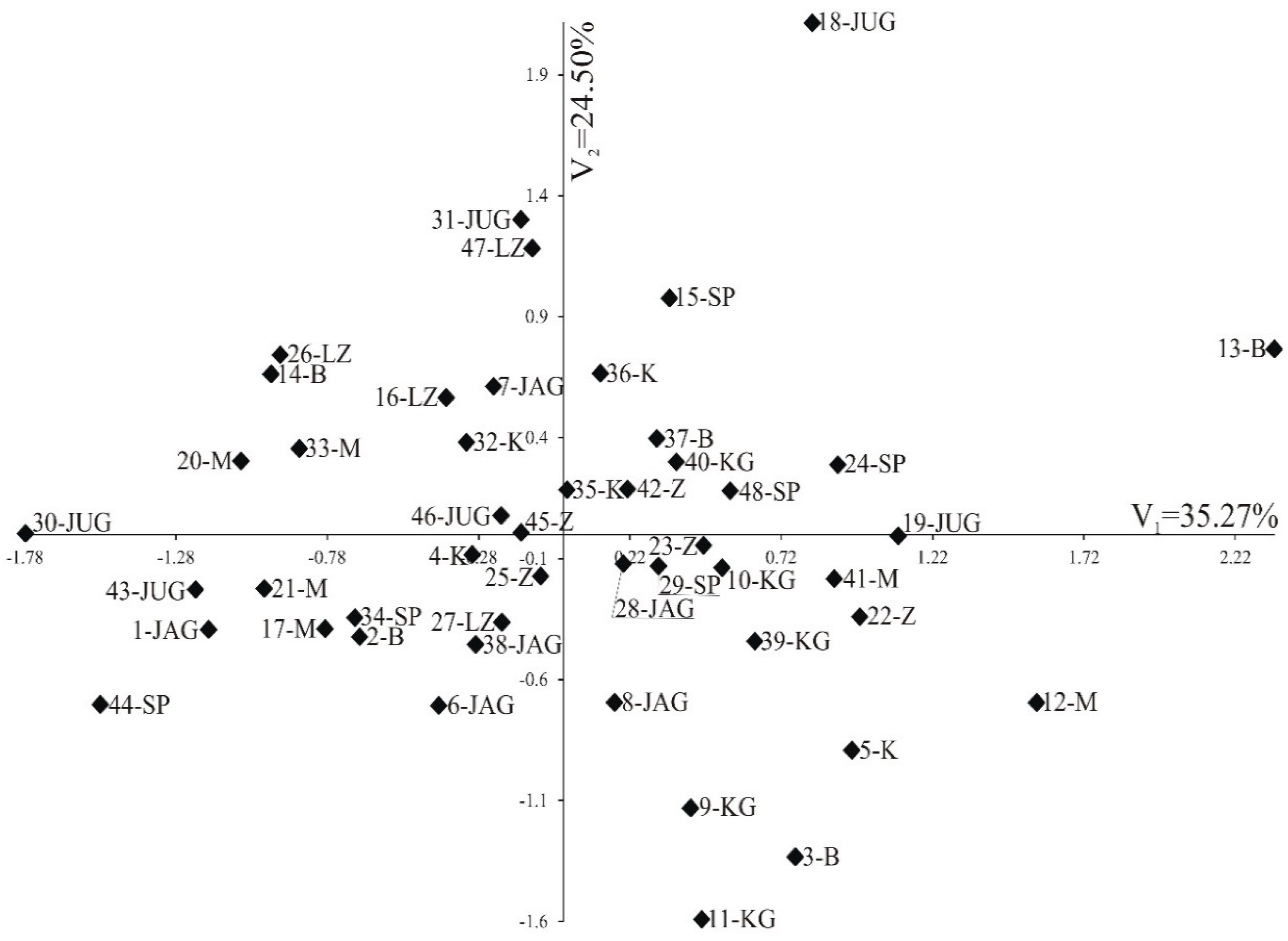
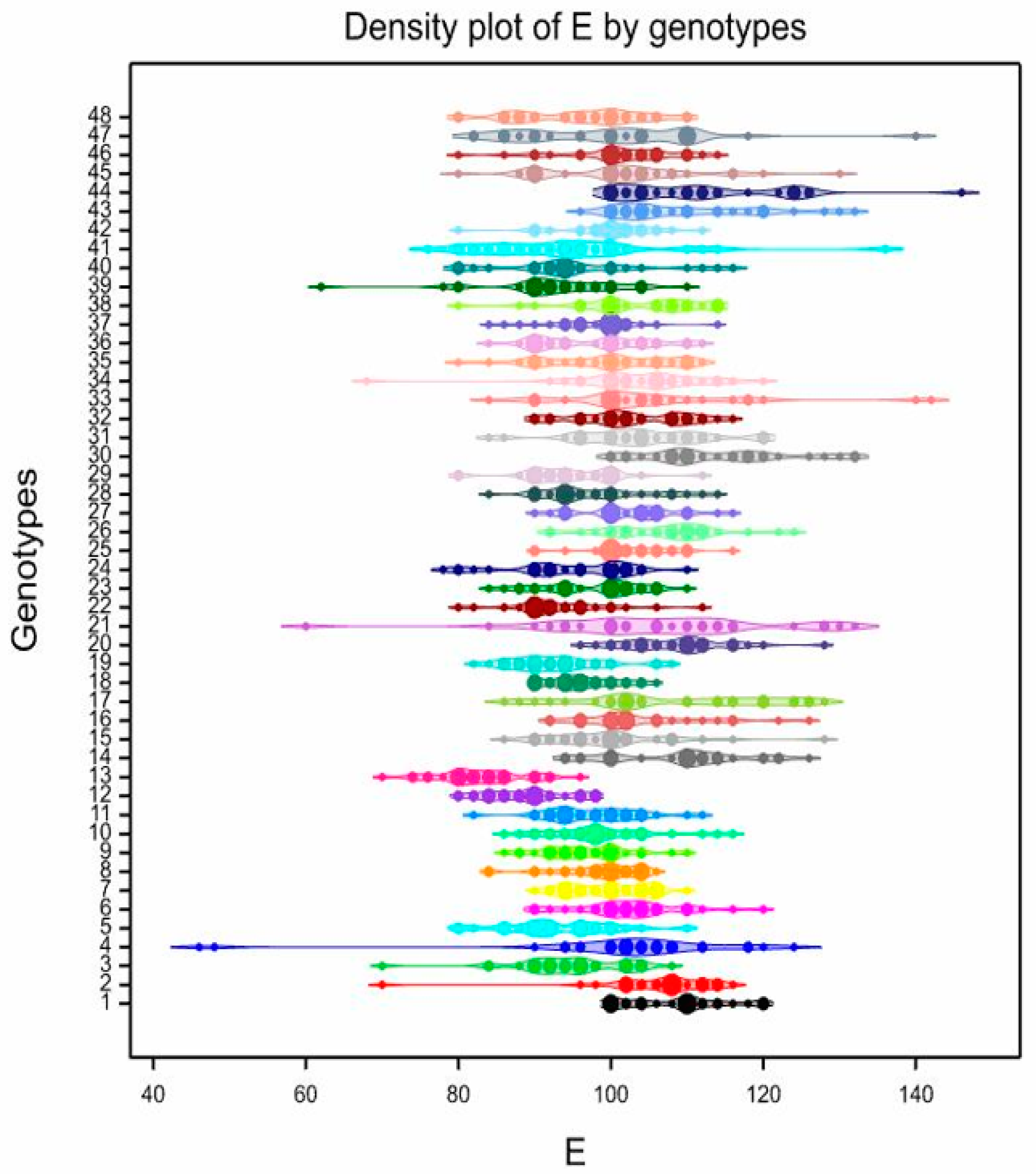
3.3. Pollen Variability of the Studied Genotypes
4. Discussion
5. Conclusions
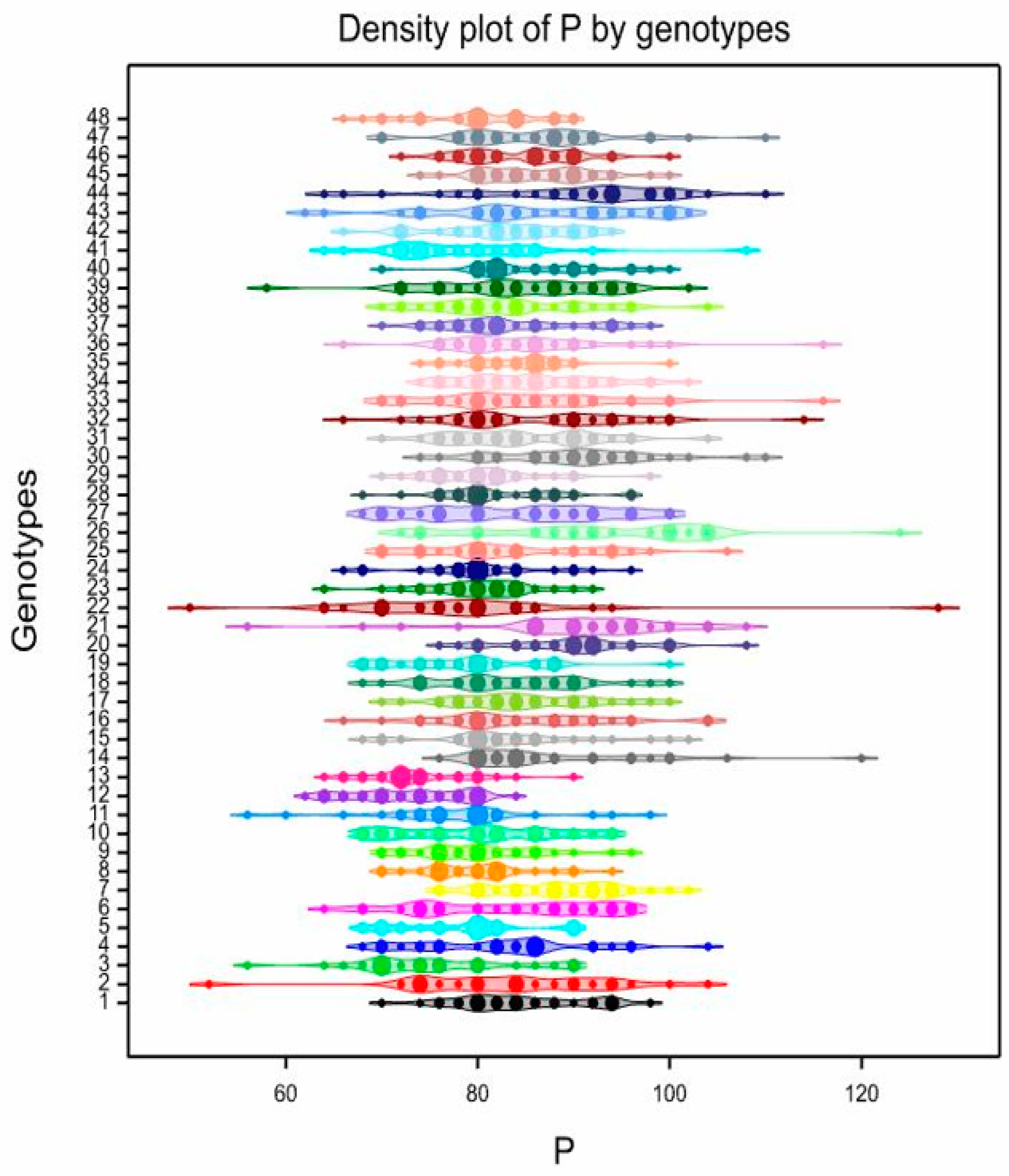
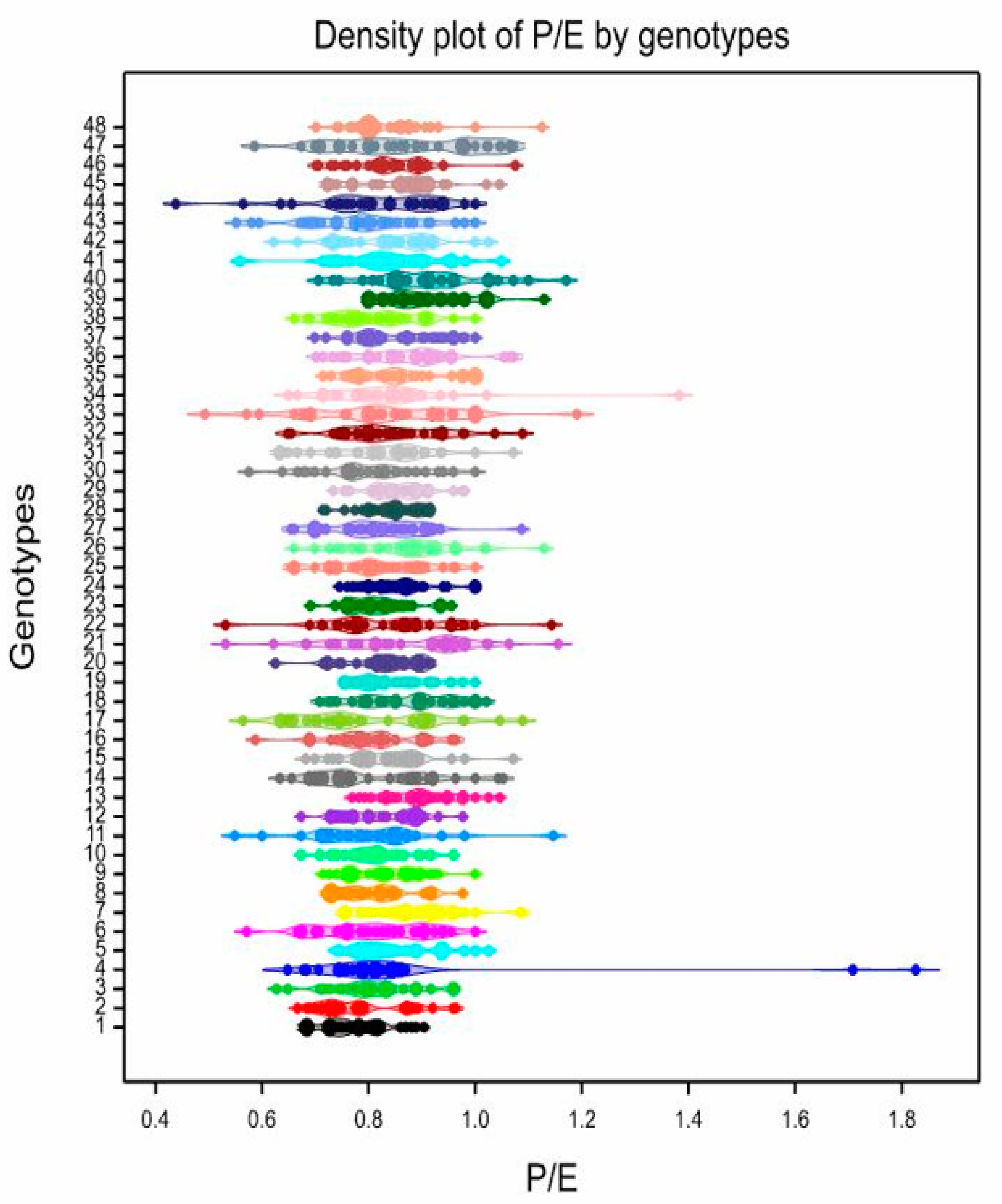
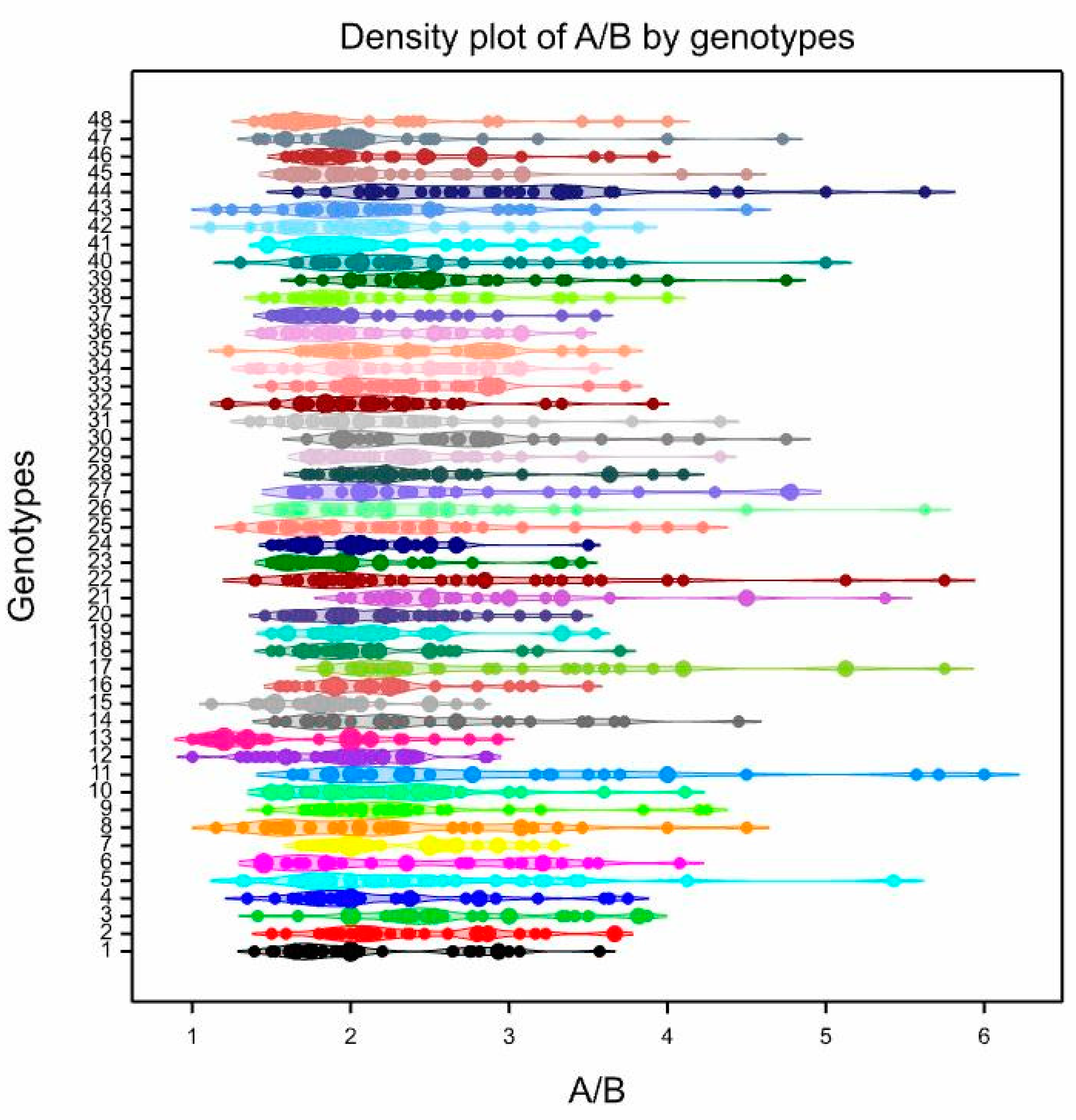
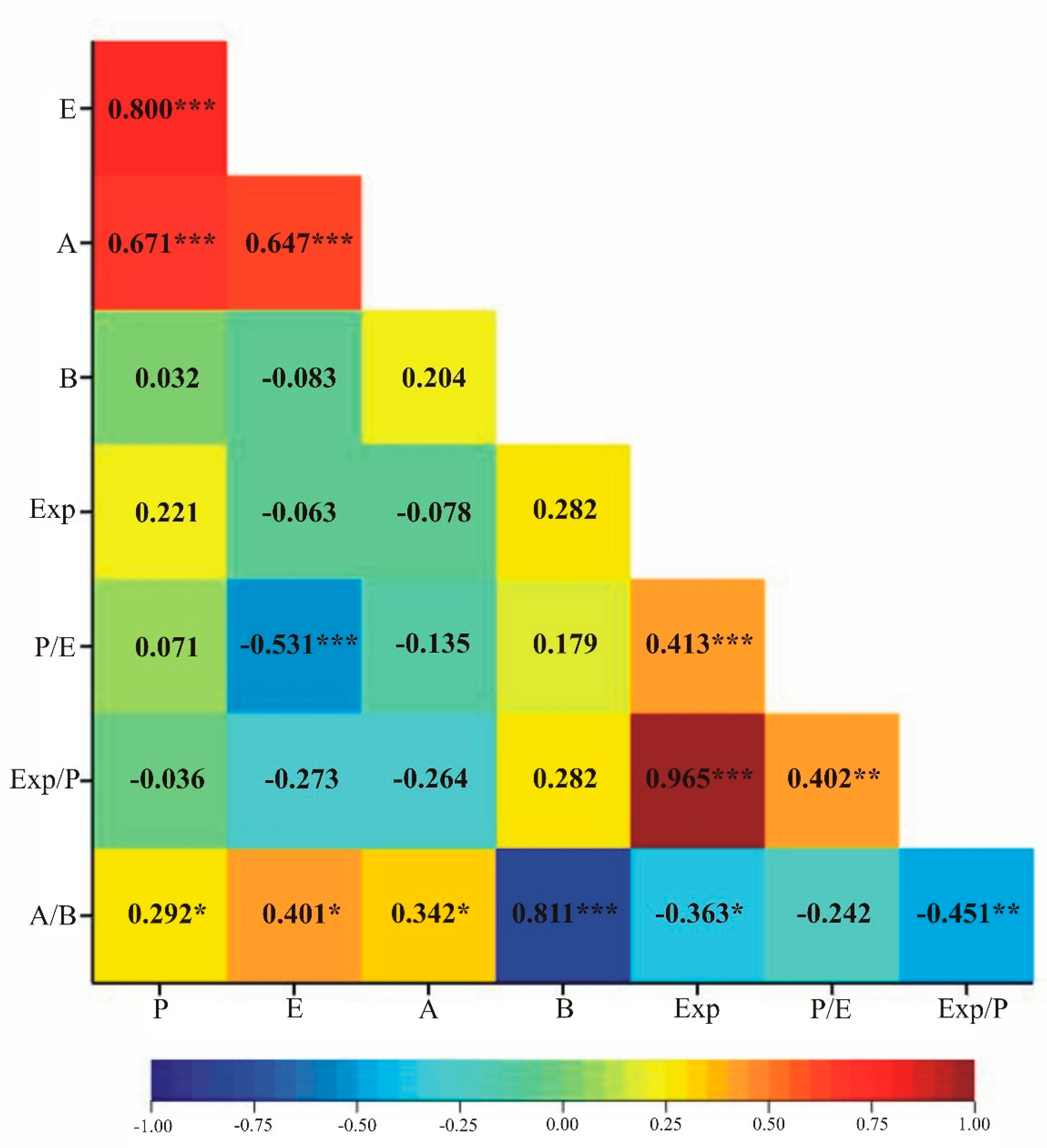
- The most important pollen grain features of the studied Abies alba genotypes are comprised of exine surface of pollen corpus (cappa and leptoma) and sacci, the length of the polar axis (P), pollen shape (P/E ratio), and the new trait, saccus shape (A/B ratio).
- The results of the presented study showed that the analysed morphological features of pollen grains from 48 A. alba genotypes did not provide grounds to distinguish individual genotypes, except for a few of them, but were generally their groups.
- Nevertheless, in our opinion the pollen of A. alba was the source of important characteristics at the species and genotype level. These results of the first study on the pollen morphology and variability of A. alba, could support further research on the reproduction of this valuable forest tree species.
Author Contributions
Funding
Acknowledgments
Conflicts of Interest
Appendix A

| Number | Genotype Number | Object/Seed Orchard Location | ||||||||||||
|---|---|---|---|---|---|---|---|---|---|---|---|---|---|---|
| 1 | 40,077 | Karkonosze National Park | ||||||||||||
| Jagniątków | 224 | 224 | 118 | 128 | 168 | 168 | 160 | 226 | 164 | 178 | 132 | 150 | ||
| 2 | 4064 | Forest District Bystrzyca Kłodzka | ||||||||||||
| Pokrzywno | 221 | 224 | 108 | 108 | 168 | 168 | 244 | 260 | 170 | 176 | 140 | 152 | ||
| 3 | 4144 | Forest District Bystrzyca Kłodzka | ||||||||||||
| Pokrzywno | 224 | 224 | 108 | 112 | 172 | 172 | 238 | 264 | 154 | 168 | 150 | 150 | ||
| 4 | 20,011 | Karkonosze National Park | ||||||||||||
| Karpacz | 224 | 224 | 110 | 116 | 170 | 172 | 160 | 236 | 166 | 194 | 146 | 146 | ||
| 5 | 10,041 | Karkonosze National Park | ||||||||||||
| Karpacz | 221 | 224 | 110 | 110 | 170 | 170 | 174 | 236 | 152 | 186 | 154 | 154 | ||
| 6 | 40,019 | Karkonosze National Park | ||||||||||||
| Jagniątków | 224 | 221 | 110 | 110 | 168 | 178 | 248 | 248 | 166 | 168 | 150 | 152 | ||
| 7 | 40,036 | Karkonosze National Park | ||||||||||||
| Jagniątków | 224 | 224 | 110 | 110 | 170 | 172 | 206 | 240 | 154 | 166 | 132 | 152 | ||
| 8 | 40,056 | Karkonosze National Park | ||||||||||||
| Jagniątków | 221 | 224 | 108 | 116 | 172 | 176 | 240 | 248 | 165 | 168 | 140 | 152 | ||
| 9 | 87 | Forest District Kamienna Góra | ||||||||||||
| Ogorzelec | 224 | 224 | 110 | 110 | 168 | 168 | 206 | 248 | 162 | 162 | 140 | 154 | ||
| 10 | 142 | Forest District Kamienna Góra | ||||||||||||
| Ogorzelec | - | - | 108 | 114 | 172 | 172 | 234 | 234 | 170 | 170 | 150 | 150 | ||
| 11 | 127 | Forest District Kamienna Góra | ||||||||||||
| Ogorzelec | 224 | 224 | 112 | 112 | 168 | 168 | 176 | 178 | 172 | 194 | 150 | 150 | ||
| 12 | 24 | Forest District Śnieżka | ||||||||||||
| Maciejowa | - | - | 110 | 112 | 168 | 170 | 206 | 248 | 172 | 186 | 150 | 150 | ||
| 13 | 4063 | Forest District Bystrzyca Kłodzka | ||||||||||||
| Pokrzywno | 224 | 224 | 110 | 110 | 168 | 168 | 188 | 206 | 154 | 166 | 140 | 148 | ||
| 14 | 4002 | Forest District Bystrzyca Kłodzka | ||||||||||||
| Pokrzywno | 224 | 224 | 110 | 110 | 168 | 178 | 236 | 240 | 152 | 170 | 148 | 148 | ||
| 15 | 60,046 | Karkonosze National Park | ||||||||||||
| Szklarska Poręba | 224 | 224 | 108 | 114 | 168 | 170 | 160 | 250 | 170 | 172 | 150 | 152 | ||
| 16 | 3021 | Forest District Lądek Zdrój | ||||||||||||
| Trzebieszowice | 206 | 221 | 110 | 110 | 176 | 176 | 174 | 246 | 152 | 170 | 140 | 140 | ||
| 17 | 198 | Forest District Śnieżka | ||||||||||||
| Maciejowa | - | - | 108 | 108 | 168 | 170 | 174 | 248 | 170 | 178 | 140 | 140 | ||
| 18 | 5341 | Forest District Jugów | ||||||||||||
| Wojbórz | 224 | 224 | 110 | 110 | 168 | 168 | 174 | 236 | 152 | 152 | 150 | 160 | ||
| 19 | 5335 | Forest District Jugów | ||||||||||||
| Wojbórz | 221 | 224 | 110 | 116 | 168 | 168 | 160 | 160 | 172 | 172 | 142 | 142 | ||
| 20 | 12 | Forest District Śnieżka | ||||||||||||
| Maciejowa | - | - | 110 | 110 | 168 | 170 | 160 | 206 | 170 | 194 | 138 | 148 | ||
| 21 | 235 | Forest District Śnieżka | ||||||||||||
| Maciejowa | - | - | 110 | 110 | 170 | 170 | 242 | 248 | 166 | 168 | 152 | 152 | ||
| 22 | 6031 | Forest District Zdroje | ||||||||||||
| Duszniki | 224 | 224 | 108 | 110 | 170 | 170 | 168 | 236 | 186 | 186 | 142 | 150 | ||
| 23 | 6078 | Forest District Zdroje | ||||||||||||
| Duszniki | 221 | 221 | 110 | 110 | 168 | 178 | 240 | 240 | 154 | 154 | 150 | 152 | ||
| 24 | 60,017 | Karkonosze National Park | ||||||||||||
| Szklarska Poręba | 221 | 224 | 108 | 108 | 168 | 168 | 242 | 248 | 166 | 176 | 152 | 152 | ||
| 25 | 6074 | Forest District Zdroje | ||||||||||||
| Duszniki | 224 | 224 | 110 | 112 | 168 | 176 | 250 | 250 | 166 | 166 | 142 | 142 | ||
| 26 | 3014 | Forest District Lądek Zdrój | ||||||||||||
| Trzebieszowice | 224 | 224 | 110 | 110 | 170 | 172 | 194 | 194 | 166 | 178 | 140 | 140 | ||
| 27 | 3158 | Forest District Lądek Zdrój | ||||||||||||
| Trzebieszowice | 221 | 221 | 112 | 112 | 168 | 176 | 240 | 248 | 152 | 170 | 140 | 140 | ||
| 28 | 40,073 | Karkonosze National Park | ||||||||||||
| Jagniątków | 224 | 224 | 110 | 116 | 168 | 170 | 174 | 242 | 168 | 168 | 140 | 152 | ||
| 29 | 60,135 | Karkonosze National Park | ||||||||||||
| Szklarska Poręba | 221 | 224 | 110 | 110 | 168 | 170 | 160 | 250 | 154 | 192 | 150 | 152 | ||
| 30 | 5347 | Forest District Jugów | ||||||||||||
| Wojbórz | 224 | 224 | 110 | 110 | 168 | 174 | 194 | 226 | 166 | 166 | 150 | 150 | ||
| 31 | 5262 | Forest District Jugów | ||||||||||||
| Wojbórz | 221 | 224 | 110 | 110 | 172 | 172 | 174 | 174 | 152 | 170 | 152 | 152 | ||
| 32 | 10,038 | Karkonosze National Park | ||||||||||||
| Karpacz | 221 | 224 | 108 | 108 | 168 | 170 | 194 | 250 | 152 | 194 | 140 | 144 | ||
| 33 | 78 | Forest District Śnieżka | ||||||||||||
| Maciejowa | 221 | 224 | 110 | 112 | 170 | 172 | 226 | 250 | 170 | 178 | 150 | 150 | ||
| 34 | 60,002 | Karkonosze National Park | ||||||||||||
| Szklarska Poręba | 221 | 224 | - | - | 172 | 172 | 178 | 242 | 178 | 178 | 148 | 154 | ||
| 35 | 30,006 | Karkonosze National Park | ||||||||||||
| Karpacz | 224 | 224 | 110 | 116 | 168 | 172 | 174 | 246 | 152 | 178 | 140 | 140 | ||
| 36 | 20,019 | Karkonosze National Park | ||||||||||||
| Karpacz | 224 | 224 | 110 | 110 | 168 | 168 | 242 | 250 | 152 | 178 | 140 | 146 | ||
| 37 | 4122 | Forest District Bystrzyca Kłodzka | ||||||||||||
| Pokrzywno | 224 | 224 | 110 | 110 | 174 | 174 | 206 | 226 | 166 | 196 | 140 | 152 | ||
| 38 | 40,049 | Karkonosze National Park Jagniątków | ||||||||||||
| 224 | 224 | 110 | 110 | 172 | 172 | 242 | 250 | 152 | 166 | 132 | 152 | |||
| 39 | 65 | Forest District Kamienna Góra | ||||||||||||
| Ogorzelec | 224 | 224 | 110 | 110 | 172 | 172 | 236 | 236 | 186 | 186 | 146 | 152 | ||
| 40 | 15 | Forest District Kamienna Góra | ||||||||||||
| Ogorzelec | 221 | 224 | 110 | 110 | 168 | 168 | 236 | 250 | 166 | 166 | 146 | 146 | ||
| 41 | 133 | Forest District Śnieżka | ||||||||||||
| Maciejowa | - | - | 108 | 116 | 168 | 168 | 160 | 160 | 164 | 164 | 146 | 152 | ||
| 42 | 6056 | Forest District Zdroje | ||||||||||||
| Duszniki | 224 | 224 | 110 | 112 | 172 | 172 | 206 | 248 | 168 | 170 | 144 | 144 | ||
| 43 | 5254 | Forest District Jugów | ||||||||||||
| Wojbórz | 206 | 221 | 110 | 110 | 172 | 178 | 178 | 236 | 166 | 172 | 148 | 156 | ||
| 44 | 60,086 | Karkonosze National Park | ||||||||||||
| Szklarska Poręba | 224 | 224 | 110 | 110 | 170 | 170 | 240 | 250 | 178 | 178 | 152 | 152 | ||
| 45 | 6094 | Forest District Zdroje | ||||||||||||
| Duszniki | 224 | 224 | 114 | 114 | 172 | 172 | 248 | 248 | 176 | 176 | 150 | 150 | ||
| 46 | 5314 | Forest District Jugów | ||||||||||||
| Wojbórz | 224 | 224 | 108 | 116 | 168 | 170 | 206 | 206 | 152 | 172 | 140 | 140 | ||
| 47 | 3125 | Forest District Lądek Zdrój | ||||||||||||
| Trzebieszowice | 224 | 224 | 110 | 110 | 168 | 170 | 164 | 250 | 176 | 176 | 140 | 140 | ||
| 48 | 60,206 | Karkonosze National Park | ||||||||||||
| Szklarska Poręba | 224 | 224 | 110 | 110 | 168 | 170 | 160 | 160 | 180 | 180 | 140 | 150 |
| Genotype | P | E | A | B | ||||||||||||
|---|---|---|---|---|---|---|---|---|---|---|---|---|---|---|---|---|
| Mean | Range | cv | Mean | Range | cv | Mean | Range | cv | Mean | Range | cv | |||||
| 1 | 84.33 | bcdefghi | 70–98 | 8.19 | 108.5 | abcde | 100–120 | 6.01 | 82.27 | a | 64–104 | 13.67 | 39.53 | ab | 28–50 | 15.13 |
| 2 | 83.53 | bcdefghi | 52–104 | 12.41 | 106.1 | bcdefghi | 70–116 | 7.90 | 76.07 | abcdefghij | 56–92 | 12.09 | 32.33 | cdefghijklmn | 24–44 | 16.73 |
| 3 | 75.47 | jkl | 56–90 | 10.85 | 94.7 | opqr | 70–108 | 8.04 | 71 | fghijklmn | 56–86 | 11.69 | 28 | mno | 16–48 | 23.73 |
| 4 | 82.6 | efghi | 68–104 | 10.77 | 101.1 | fghijklmno | 46–124 | 16.50 | 71.33 | efghijklmn | 60–90 | 12.37 | 33.13 | cdefghijklm | 20–52 | 22.79 |
| 5 | 78.33 | hijkl | 68–90 | 8.32 | 93 | pqr | 80–110 | 7.51 | 67.33 | klmn | 42–84 | 12.99 | 30 | ijklmno | 14–54 | 26.95 |
| 6 | 83 | defghi | 64–96 | 11.49 | 102.7 | defghijklm | 90–120 | 6.78 | 76.67 | abcdefghi | 58–114 | 20.25 | 33.47 | cdefghijklm | 22–44 | 19.15 |
| 7 | 88.4 | abcde | 76–102 | 7.71 | 99.6 | ghijklmnopq | 90–110 | 5.31 | 79.07 | abcd | 60–92 | 11.05 | 34.53 | bcdefghijk | 26–50 | 17.99 |
| 8 | 80 | fghijkl | 70–94 | 7.19 | 98.3 | jklmnopq | 84–106 | 5.82 | 76.07 | abcdefghij | 62–90 | 10.91 | 35.8 | bcdefghi | 20–54 | 24.70 |
| 9 | 80.27 | fghijk | 70–96 | 8.11 | 96.8 | klmnopq | 86–110 | 5.91 | 68.73 | jklmn | 52–100 | 15.80 | 30.47 | ghijklmno | 16–46 | 18.86 |
| 10 | 80 | fghijkl | 68–94 | 10.13 | 98.8 | ijklmnopq | 86–116 | 7.26 | 65.73 | lmn | 48–82 | 12.55 | 30.33 | hijklmno | 18–44 | 19.67 |
| 11 | 77.8 | ijkl | 56–98 | 11.08 | 97.8 | klmnopq | 82–112 | 6.50 | 70.27 | hijklmn | 58–80 | 9.80 | 26.27 | o | 12–38 | 29.23 |
| 12 | 73.07 | l | 62–84 | 8.28 | 89.1 | rs | 80–98 | 6.00 | 65.2 | mn | 52–80 | 12.31 | 34.27 | bcdefghijkl | 26–56 | 16.84 |
| 13 | 73.93 | kl | 64–90 | 7.67 | 82.9 | s | 70–96 | 7.19 | 64.4 | n | 54–86 | 11.22 | 43 | a | 24–60 | 27.90 |
| 14 | 87.8 | abcde | 76–120 | 10.99 | 108.9 | abcd | 94–126 | 8.08 | 76.73 | abcdefghi | 64–98 | 12.37 | 33.07 | cdefghijklm | 22–44 | 21.94 |
| 15 | 83.2 | cdefghi | 68–102 | 9.95 | 100.1 | ghijklmnop | 86–128 | 8.68 | 67.67 | klmn | 50–90 | 11.28 | 37.6 | abcd | 24–50 | 17.24 |
| 16 | 84.53 | bcdefghi | 66–104 | 10.74 | 104.1 | cdefghijk | 92–126 | 7.96 | 75.47 | abcdefghij | 64–90 | 10.69 | 35.33 | bcdefghij | 24–44 | 14.82 |
| 17 | 84.67 | bcdefghi | 70–100 | 8.69 | 107.9 | abcdef | 86–128 | 11.33 | 73.53 | cdefghijk | 62–92 | 10.42 | 26.67 | no | 16–38 | 24.15 |
| 18 | 83.4 | bcdefghi | 68–100 | 9.57 | 96.2 | lmnopqr | 90–106 | 4.71 | 69.4 | ijklmn | 56–84 | 9.99 | 33.47 | cdefghijklm | 20–40 | 15.21 |
| 19 | 78.8 | ghijkl | 68–100 | 9.53 | 93.1 | pqr | 82–108 | 6.93 | 65.07 | mn | 50–80 | 13.40 | 30.73 | fghijklmno | 18–52 | 20.90 |
| 20 | 89.87 | abcd | 76–108 | 7.97 | 108.8 | abcd | 96–128 | 6.43 | 76 | abcdefghij | 60–96 | 11.63 | 35.4 | bcdefghij | 26–48 | 16.60 |
| 21 | 90.13 | abc | 56–108 | 11.98 | 106.2 | bcdefgh | 60–132 | 14.20 | 77.47 | abcdefgh | 64–90 | 7.70 | 29.4 | klmno | 16–36 | 20.62 |
| 22 | 78.13 | hijkl | 50–128 | 16.63 | 93.2 | pqr | 80–112 | 6.96 | 71.8 | defghijklmn | 56–92 | 13.21 | 29.87 | jklmno | 16–46 | 25.96 |
| 23 | 80.13 | fghijk | 64–92 | 7.27 | 97.6 | klmnopq | 84–110 | 6.82 | 70.47 | ghijklmn | 60–86 | 8.15 | 36.27 | bcdefg | 20–48 | 19.68 |
| 24 | 80.4 | fghijk | 66–96 | 8.27 | 94.7 | opqr | 78–110 | 8.54 | 65.2 | mn | 54–84 | 11.49 | 31.93 | defghijklmno | 24–44 | 18.50 |
| 25 | 83.53 | bcdefghi | 70–106 | 10.83 | 102.3 | defghijklmn | 90–116 | 5.53 | 70.2 | hijklmn | 60–94 | 11.70 | 32.93 | cdefghijklm | 18–50 | 25.46 |
| 26 | 92.53 | a | 72–124 | 12.87 | 106.9 | abcdefg | 92–124 | 7.20 | 78.93 | abcde | 62–96 | 12.41 | 35.13 | bcdefghijk | 16–46 | 20.37 |
| 27 | 83.67 | bcdefghi | 68–100 | 11.44 | 102.3 | defghijklmn | 90–116 | 6.18 | 74.87 | abcdefghijk | 60–92 | 12.70 | 31.07 | efghijklmno | 16–44 | 24.07 |
| 28 | 82.13 | efghij | 68–96 | 7.73 | 98 | klmnopq | 84–114 | 7.47 | 75.8 | abcdefghij | 60–90 | 9.58 | 32.33 | cdefghijklmn | 20–42 | 19.84 |
| 29 | 80.6 | fghijk | 70–98 | 7.26 | 94.6 | opqr | 80–112 | 6.92 | 82.4 | a | 64–104 | 10.99 | 36.27 | bcdefg | 24–48 | 18.24 |
| 30 | 90.33 | ab | 74–110 | 9.47 | 113.9 | a | 100–132 | 8.16 | 80.93 | abc | 64–96 | 8.87 | 31.87 | defghijklmno | 16–44 | 19.36 |
| 31 | 84.87 | bcdefgh | 70–104 | 9.11 | 104.1 | cdefghijk | 84–120 | 8.54 | 70.8 | fghijklmn | 60–92 | 12.40 | 33.67 | bcdefghijklm | 18–44 | 19.80 |
| 32 | 86.4 | abcdef | 66–114 | 11.60 | 102.7 | defghijklm | 90–116 | 7.00 | 74.73 | abcdefghijk | 56–92 | 12.22 | 35.87 | bcdefgh | 22–52 | 18.34 |
| 33 | 85.13 | bcdefgh | 70–116 | 11.91 | 105.5 | bcdefghij | 84–142 | 12.23 | 81.6 | ab | 64–112 | 15.22 | 35.27 | bcdefghij | 24–48 | 18.33 |
| 34 | 85.73 | abcdefg | 74–102 | 8.39 | 103.5 | cdefghijkl | 68–120 | 9.08 | 78.93 | abcde | 60–100 | 14.44 | 35.13 | bcdefghijk | 26–46 | 14.70 |
| 35 | 84.07 | bcdefghi | 74–100 | 6.17 | 99.1 | hijklmnopq | 80–112 | 8.49 | 76.2 | abcdefghij | 56–90 | 11.52 | 33 | cdefghijklm | 20–62 | 23.75 |
| 36 | 85.07 | bcdefgh | 66–116 | 10.88 | 97.5 | klmnopq | 84–112 | 7.66 | 78.13 | abcdefg | 66–118 | 15.28 | 37.07 | bcd | 22–48 | 17.68 |
| 37 | 83.47 | bcdefghi | 70–98 | 8.56 | 97.8 | klmnopq | 84–114 | 6.16 | 72.33 | defghijklm | 60–88 | 10.53 | 36.4 | bcdef | 22–46 | 15.57 |
| 38 | 83.47 | bcdefghi | 70–104 | 9.60 | 103.2 | cdefghijklm | 80–114 | 8.01 | 71.53 | defghijklmn | 54–102 | 16.17 | 31.8 | defghijklmno | 20–42 | 16.79 |
| 39 | 84.27 | bcdefghi | 58–102 | 11.04 | 92.6 | qr | 62–110 | 9.99 | 72.13 | defghijklmn | 58–88 | 10.24 | 28.53 | lmno | 16–40 | 18.77 |
| 40 | 85.8 | abcdefg | 70–100 | 7.70 | 95.1 | nopqr | 80–116 | 9.95 | 73.4 | cdefghijkl | 54–90 | 12.44 | 32.47 | cdefghijklmn | 14–46 | 24.51 |
| 41 | 78.4 | hijkl | 64–108 | 10.87 | 94.6 | opqr | 76–136 | 12.93 | 65.27 | mn | 50–90 | 15.53 | 30.8 | fghijklmno | 18–42 | 20.58 |
| 42 | 82.6 | efghi | 66–94 | 8.51 | 99.3 | hijklmnopq | 80–112 | 6.31 | 70.87 | fghijklmn | 40–84 | 13.84 | 34.8 | bcdefghijk | 20–46 | 18.21 |
| 43 | 86 | abcdef | 62–102 | 12.61 | 110.3 | abc | 96–132 | 8.97 | 77.2 | abcdefgh | 60–102 | 13.82 | 36.87 | bcde | 20–52 | 21.45 |
| 44 | 89.93 | abcd | 64–110 | 12.37 | 112.1 | ab | 100–146 | 9.81 | 78.33 | abcdef | 60–96 | 11.81 | 27.87 | mno | 16–48 | 24.93 |
| 45 | 86.27 | abcdef | 74–100 | 7.20 | 101.3 | efghijklmno | 80–130 | 10.50 | 71 | fghijklmn | 54–90 | 12.44 | 33.4 | cdefghijklm | 20–48 | 22.69 |
| 46 | 84.47 | bcdefghi | 72–100 | 7.48 | 100.9 | fghijklmno | 80–114 | 7.61 | 77.27 | abcdefgh | 66–92 | 8.90 | 36.2 | bcdefg | 22–46 | 19.65 |
| 47 | 86.33 | abcdef | 70–110 | 10.07 | 100.3 | ghijklmnop | 82–140 | 12.37 | 76.33 | abcdefghij | 64–104 | 11.29 | 37.33 | abcd | 22–54 | 22.87 |
| 48 | 79.73 | fghijkl | 66–90 | 8.09 | 95.9 | mnopqr | 80–110 | 8.58 | 73.87 | bcdefghijk | 64–96 | 11.68 | 37.87 | abc | 22–48 | 18.34 |
| LSD0.001 | 7.053 | 7.337 | 7.739 | 5.863 | ||||||||||||
| ANOVA F | 7.72 *** | 15.42 *** | 8.70 *** | 7.30 *** | ||||||||||||
| Genotype | 1 | 2 | 3 | 4 | 5 | 6 | 7 | 8 | 9 | 10 | 11 | 12 | 13 | 14 | 15 | 16 | 17 | 18 | 19 | 20 | 21 | 22 | 23 | |
|---|---|---|---|---|---|---|---|---|---|---|---|---|---|---|---|---|---|---|---|---|---|---|---|---|
| 2 | 1.63 | |||||||||||||||||||||||
| 3 | 2.73 | 1.91 | ||||||||||||||||||||||
| 4 | 2.35 | 1.65 | 2.35 | |||||||||||||||||||||
| 5 | 2.77 | 1.97 | 0.94 | 2.01 | ||||||||||||||||||||
| 6 | 1.33 | 0.72 | 1.64 | 1.71 | 1.65 | |||||||||||||||||||
| 7 | 1.97 | 1.68 | 2.40 | 1.98 | 2.13 | 1.58 | ||||||||||||||||||
| 8 | 1.48 | 1.53 | 1.54 | 2.05 | 1.48 | 0.91 | 1.69 | |||||||||||||||||
| 9 | 2.43 | 1.66 | 1.08 | 1.99 | 0.76 | 1.30 | 2.06 | 1.40 | ||||||||||||||||
| 10 | 2.86 | 1.53 | 1.67 | 1.82 | 1.32 | 1.73 | 1.98 | 2.03 | 1.44 | |||||||||||||||
| 11 | 2.90 | 2.26 | 1.19 | 2.42 | 1.29 | 1.99 | 2.79 | 1.86 | 1.49 | 2.08 | ||||||||||||||
| 12 | 2.99 | 2.35 | 1.34 | 2.48 | 1.03 | 2.02 | 2.40 | 1.66 | 1.41 | 1.68 | 2.10 | |||||||||||||
| 13 | 4.11 | 3.89 | 3.68 | 3.53 | 3.15 | 3.65 | 3.56 | 3.14 | 3.66 | 3.36 | 3.87 | 2.71 | ||||||||||||
| 14 | 2.11 | 1.30 | 2.73 | 1.69 | 2.56 | 1.75 | 1.50 | 2.25 | 2.47 | 1.84 | 2.85 | 3.01 | 3.99 | |||||||||||
| 15 | 2.62 | 1.94 | 2.64 | 1.91 | 2.10 | 2.05 | 1.56 | 2.12 | 2.25 | 1.45 | 2.88 | 2.22 | 2.80 | 1.56 | ||||||||||
| 16 | 1.82 | 1.13 | 2.29 | 1.68 | 2.10 | 1.36 | 0.95 | 1.68 | 2.04 | 1.54 | 2.65 | 2.36 | 3.51 | 0.84 | 1.16 | |||||||||
| 17 | 2.67 | 1.73 | 2.31 | 1.66 | 2.24 | 2.00 | 2.37 | 2.42 | 2.24 | 1.90 | 1.92 | 3.03 | 4.31 | 1.53 | 2.36 | 1.91 | ||||||||
| 18 | 4.00 | 3.22 | 3.53 | 3.06 | 3.20 | 3.46 | 2.40 | 3.49 | 3.53 | 2.48 | 3.89 | 3.25 | 3.65 | 2.46 | 1.92 | 2.27 | 3.16 | |||||||
| 19 | 3.21 | 1.98 | 1.83 | 2.09 | 1.41 | 2.07 | 2.16 | 2.21 | 1.71 | 0.76 | 2.41 | 1.43 | 2.94 | 2.32 | 1.60 | 1.90 | 2.49 | 2.45 | ||||||
| 20 | 1.72 | 1.14 | 2.78 | 1.82 | 2.50 | 1.40 | 1.50 | 2.02 | 2.19 | 1.95 | 2.93 | 2.91 | 3.98 | 1.04 | 1.66 | 1.10 | 2.05 | 3.09 | 2.39 | |||||
| 21 | 2.02 | 1.16 | 2.36 | 1.38 | 2.14 | 1.34 | 1.63 | 1.98 | 1.90 | 1.84 | 2.30 | 2.85 | 4.12 | 1.17 | 2.04 | 1.43 | 1.27 | 3.19 | 2.32 | 1.11 | ||||
| 22 | 2.82 | 1.85 | 1.35 | 2.15 | 1.25 | 1.77 | 2.07 | 1.64 | 1.73 | 1.32 | 1.82 | 1.40 | 2.75 | 2.29 | 1.91 | 1.86 | 2.24 | 2.72 | 1.19 | 2.50 | 2.23 | |||
| 23 | 1.97 | 1.46 | 1.66 | 1.73 | 1.23 | 1.19 | 1.35 | 0.99 | 1.32 | 1.31 | 2.06 | 1.35 | 2.78 | 1.85 | 1.21 | 1.18 | 2.23 | 2.69 | 1.48 | 1.71 | 1.84 | 1.35 | ||
| 24 | 3.07 | 1.92 | 1.97 | 1.90 | 1.44 | 2.02 | 1.87 | 2.16 | 1.71 | 0.68 | 2.46 | 1.57 | 2.98 | 2.04 | 1.22 | 1.62 | 2.34 | 2.13 | 0.50 | 2.15 | 2.13 | 1.38 | 1.30 | |
| 25 | 2.04 | 1.09 | 1.78 | 1.47 | 1.35 | 1.10 | 1.49 | 1.43 | 1.27 | 1.00 | 1.88 | 1.91 | 3.34 | 1.37 | 1.26 | 1.09 | 1.57 | 2.76 | 1.52 | 1.25 | 1.19 | 1.55 | 0.88 | |
| 26 | 1.91 | 1.64 | 2.94 | 2.11 | 2.60 | 1.75 | 1.13 | 2.09 | 2.45 | 2.19 | 3.02 | 3.04 | 3.86 | 1.07 | 1.57 | 1.09 | 2.16 | 2.74 | 2.56 | 0.85 | 1.34 | 2.51 | 1.77 | |
| 27 | 1.88 | 0.81 | 1.58 | 1.57 | 1.45 | 0.85 | 1.49 | 1.24 | 1.40 | 1.25 | 1.72 | 2.01 | 3.43 | 1.34 | 1.64 | 1.11 | 1.45 | 2.91 | 1.68 | 1.39 | 1.10 | 1.29 | 1.08 | |
| 28 | 1.98 | 1.08 | 1.49 | 1.74 | 1.42 | 0.99 | 1.18 | 1.16 | 1.45 | 1.29 | 2.08 | 1.64 | 3.20 | 1.61 | 1.59 | 1.02 | 2.04 | 2.64 | 1.43 | 1.67 | 1.58 | 1.09 | 0.89 | |
| 29 | 1.87 | 2.00 | 2.07 | 2.52 | 2.19 | 1.61 | 1.58 | 1.23 | 2.22 | 2.53 | 2.74 | 2.05 | 3.26 | 2.50 | 2.44 | 1.84 | 3.03 | 3.28 | 2.49 | 2.46 | 2.50 | 1.90 | 1.60 | |
| 30 | 1.80 | 1.31 | 2.96 | 1.95 | 2.93 | 1.70 | 2.02 | 2.41 | 2.62 | 2.45 | 2.95 | 3.49 | 4.69 | 1.07 | 2.44 | 1.57 | 1.64 | 3.50 | 2.99 | 1.13 | 1.06 | 2.86 | 2.37 | |
| 31 | 2.95 | 2.07 | 2.92 | 2.02 | 2.59 | 2.43 | 1.74 | 2.69 | 2.74 | 1.70 | 3.12 | 2.89 | 3.63 | 1.14 | 1.14 | 1.22 | 2.00 | 1.41 | 2.02 | 1.87 | 2.00 | 2.24 | 1.94 | |
| 32 | 1.70 | 1.18 | 2.27 | 1.63 | 1.91 | 1.18 | 0.86 | 1.45 | 1.79 | 1.56 | 2.53 | 2.23 | 3.32 | 1.13 | 1.10 | 0.61 | 2.02 | 2.57 | 1.88 | 0.89 | 1.29 | 1.88 | 0.95 | |
| 33 | 1.44 | 1.30 | 2.50 | 1.67 | 2.50 | 1.41 | 1.21 | 1.74 | 2.36 | 2.24 | 2.82 | 2.79 | 3.91 | 1.17 | 1.99 | 0.95 | 2.02 | 2.86 | 2.56 | 1.45 | 1.49 | 2.28 | 1.72 | |
| 34 | 1.08 | 0.98 | 2.11 | 1.61 | 2.01 | 0.63 | 1.29 | 1.15 | 1.66 | 2.04 | 2.42 | 2.36 | 3.76 | 1.61 | 2.03 | 1.25 | 2.14 | 3.40 | 2.35 | 1.19 | 1.26 | 2.14 | 1.35 | |
| 35 | 1.92 | 1.17 | 1.79 | 1.56 | 1.59 | 1.13 | 0.80 | 1.30 | 1.61 | 1.38 | 2.23 | 1.90 | 3.26 | 1.32 | 1.37 | 0.72 | 1.91 | 2.40 | 1.59 | 1.46 | 1.38 | 1.37 | 0.90 | |
| 36 | 1.91 | 1.77 | 2.36 | 2.00 | 2.08 | 1.59 | 0.66 | 1.46 | 2.14 | 2.01 | 2.80 | 2.15 | 3.00 | 1.70 | 1.41 | 1.02 | 2.57 | 2.39 | 2.06 | 1.72 | 1.94 | 1.84 | 1.12 | |
| 37 | 2.04 | 1.51 | 2.07 | 1.71 | 1.60 | 1.37 | 0.98 | 1.34 | 1.67 | 1.41 | 2.46 | 1.73 | 2.81 | 1.60 | 0.92 | 0.93 | 2.30 | 2.38 | 1.51 | 1.48 | 1.73 | 1.53 | 0.56 | |
| 38 | 1.92 | 0.85 | 1.62 | 1.44 | 1.39 | 0.88 | 1.52 | 1.43 | 1.06 | 1.13 | 1.86 | 1.97 | 3.73 | 1.45 | 1.66 | 1.18 | 1.57 | 3.02 | 1.68 | 1.26 | 1.07 | 1.73 | 1.11 | |
| 39 | 2.75 | 1.74 | 1.54 | 1.75 | 1.07 | 1.56 | 1.72 | 1.72 | 1.23 | 1.28 | 1.98 | 1.57 | 3.19 | 2.22 | 1.93 | 1.84 | 2.23 | 2.93 | 1.18 | 2.13 | 1.73 | 1.24 | 1.37 | |
| 40 | 2.42 | 1.79 | 2.00 | 1.52 | 1.45 | 1.63 | 1.02 | 1.62 | 1.63 | 1.49 | 2.26 | 1.88 | 3.01 | 1.74 | 1.33 | 1.30 | 2.08 | 2.34 | 1.57 | 1.80 | 1.56 | 1.54 | 1.06 | |
| 41 | 2.95 | 1.79 | 1.52 | 1.72 | 1.03 | 1.82 | 1.98 | 1.94 | 1.34 | 0.58 | 2.01 | 1.30 | 3.06 | 2.13 | 1.53 | 1.72 | 2.12 | 2.49 | 0.58 | 2.24 | 2.04 | 1.17 | 1.22 | |
| 42 | 2.06 | 1.29 | 1.83 | 1.50 | 1.38 | 1.23 | 1.11 | 1.34 | 1.41 | 1.08 | 2.18 | 1.68 | 3.04 | 1.44 | 0.95 | 0.84 | 1.96 | 2.40 | 1.36 | 1.40 | 1.51 | 1.44 | 0.52 | |
| 43 | 1.12 | 1.09 | 2.66 | 1.73 | 2.53 | 1.16 | 1.92 | 1.72 | 2.21 | 2.27 | 2.69 | 2.93 | 3.96 | 1.42 | 2.10 | 1.45 | 1.98 | 3.63 | 2.72 | 0.95 | 1.30 | 2.55 | 1.79 | |
| 44 | 2.40 | 1.49 | 2.87 | 2.06 | 2.83 | 1.85 | 2.67 | 2.58 | 2.56 | 2.40 | 2.66 | 3.49 | 4.62 | 1.76 | 2.78 | 2.21 | 1.58 | 3.99 | 2.90 | 1.66 | 1.21 | 2.72 | 2.61 | |
| 45 | 2.10 | 1.22 | 2.08 | 1.38 | 1.55 | 1.21 | 1.35 | 1.59 | 1.41 | 1.20 | 2.23 | 2.06 | 3.32 | 1.40 | 1.22 | 1.14 | 1.83 | 2.78 | 1.57 | 1.07 | 1.11 | 1.77 | 1.02 | |
| 46 | 1.40 | 1.10 | 2.05 | 1.70 | 1.83 | 0.86 | 1.00 | 1.00 | 1.73 | 1.75 | 2.41 | 2.04 | 3.16 | 1.47 | 1.48 | 0.88 | 2.20 | 2.88 | 1.96 | 1.23 | 1.48 | 1.68 | 0.87 | |
| 47 | 2.29 | 2.13 | 2.83 | 1.92 | 2.45 | 2.12 | 1.03 | 2.06 | 2.58 | 2.20 | 3.01 | 2.68 | 3.20 | 1.47 | 1.26 | 1.13 | 2.34 | 1.98 | 2.38 | 1.82 | 1.97 | 2.25 | 1.56 | |
| 48 | 1.92 | 1.75 | 1.92 | 1.95 | 1.63 | 1.43 | 1.34 | 0.98 | 1.81 | 1.81 | 2.35 | 1.55 | 2.53 | 2.02 | 1.43 | 1.31 | 2.53 | 2.69 | 1.83 | 1.99 | 2.14 | 1.43 | 0.64 | |
| 1 | 2 | 3 | 4 | 5 | 6 | 7 | 8 | 9 | 10 | 11 | 12 | 13 | 14 | 15 | 16 | 17 | 18 | 19 | 20 | 21 | 22 | 23 | ||
| 24 | 25 | 26 | 27 | 28 | 29 | 30 | 31 | 32 | 33 | 34 | 35 | 36 | 37 | 38 | 39 | 40 | 41 | 42 | 43 | 44 | 45 | 46 | 47 | |
| 25 | 1.31 | |||||||||||||||||||||||
| 26 | 2.25 | 1.46 | ||||||||||||||||||||||
| 27 | 1.60 | 0.67 | 1.54 | |||||||||||||||||||||
| 28 | 1.38 | 1.08 | 1.72 | 0.79 | ||||||||||||||||||||
| 29 | 2.46 | 2.18 | 2.36 | 1.88 | 1.30 | |||||||||||||||||||
| 30 | 2.79 | 1.81 | 1.46 | 1.66 | 2.08 | 2.79 | ||||||||||||||||||
| 31 | 1.65 | 1.69 | 1.69 | 1.86 | 1.89 | 2.81 | 2.19 | |||||||||||||||||
| 32 | 1.60 | 0.85 | 0.87 | 1.03 | 1.05 | 1.83 | 1.67 | 1.55 | ||||||||||||||||
| 33 | 2.35 | 1.69 | 1.45 | 1.47 | 1.37 | 1.67 | 1.38 | 1.88 | 1.22 | |||||||||||||||
| 34 | 2.21 | 1.31 | 1.47 | 1.18 | 1.20 | 1.58 | 1.53 | 2.37 | 1.02 | 1.08 | ||||||||||||||
| 35 | 1.40 | 1.00 | 1.39 | 0.86 | 0.47 | 1.42 | 1.89 | 1.58 | 0.76 | 1.11 | 1.11 | |||||||||||||
| 36 | 1.82 | 1.56 | 1.42 | 1.52 | 1.08 | 1.23 | 2.30 | 1.83 | 0.94 | 1.28 | 1.37 | 0.81 | ||||||||||||
| 37 | 1.24 | 0.97 | 1.41 | 1.18 | 0.90 | 1.63 | 2.25 | 1.65 | 0.64 | 1.55 | 1.34 | 0.72 | 0.76 | |||||||||||
| 38 | 1.51 | 0.54 | 1.61 | 0.76 | 1.08 | 2.14 | 1.65 | 1.94 | 1.02 | 1.59 | 1.10 | 1.05 | 1.70 | 1.23 | ||||||||||
| 39 | 1.22 | 1.35 | 2.22 | 1.32 | 1.13 | 2.05 | 2.62 | 2.33 | 1.63 | 2.21 | 1.76 | 1.25 | 1.76 | 1.38 | 1.35 | |||||||||
| 40 | 1.28 | 1.16 | 1.60 | 1.30 | 1.10 | 1.86 | 2.35 | 1.72 | 1.07 | 1.71 | 1.55 | 0.83 | 1.07 | 0.82 | 1.34 | 1.04 | ||||||||
| 41 | 0.55 | 1.21 | 2.41 | 1.43 | 1.28 | 2.37 | 2.75 | 1.91 | 1.69 | 2.31 | 2.09 | 1.38 | 1.94 | 1.36 | 1.32 | 1.05 | 1.31 | |||||||
| 42 | 1.08 | 0.62 | 1.45 | 0.94 | 0.83 | 1.81 | 2.06 | 1.52 | 0.65 | 1.52 | 1.29 | 0.66 | 1.06 | 0.44 | 0.88 | 1.27 | 0.82 | 1.10 | ||||||
| 43 | 2.56 | 1.44 | 1.46 | 1.40 | 1.80 | 2.36 | 1.11 | 2.36 | 1.30 | 1.39 | 1.02 | 1.69 | 1.95 | 1.78 | 1.39 | 2.38 | 2.12 | 2.48 | 1.67 | |||||
| 44 | 2.85 | 1.91 | 2.12 | 1.68 | 2.30 | 3.20 | 1.24 | 2.70 | 2.15 | 2.21 | 1.97 | 2.28 | 2.85 | 2.59 | 1.82 | 2.50 | 2.61 | 2.72 | 2.37 | 1.50 | ||||
| 45 | 1.32 | 0.52 | 1.30 | 0.96 | 1.19 | 2.22 | 1.82 | 1.74 | 0.73 | 1.70 | 1.24 | 1.03 | 1.47 | 0.89 | 0.74 | 1.25 | 1.01 | 1.34 | 0.69 | 1.46 | 1.95 | |||
| 46 | 1.80 | 1.09 | 1.27 | 0.97 | 0.80 | 1.31 | 1.82 | 1.97 | 0.63 | 1.12 | 0.75 | 0.71 | 0.81 | 0.75 | 1.17 | 1.58 | 1.21 | 1.79 | 0.86 | 1.28 | 2.21 | 1.06 | ||
| 47 | 2.01 | 1.71 | 1.35 | 1.82 | 1.67 | 2.05 | 2.25 | 1.34 | 1.19 | 1.42 | 1.85 | 1.25 | 0.95 | 1.20 | 1.95 | 2.20 | 1.24 | 2.16 | 1.33 | 2.11 | 2.92 | 1.65 | 1.42 | |
| 48 | 1.69 | 1.39 | 1.89 | 1.38 | 1.01 | 1.20 | 2.57 | 2.10 | 1.18 | 1.64 | 1.48 | 1.00 | 0.84 | 0.75 | 1.61 | 1.66 | 1.21 | 1.65 | 0.96 | 1.97 | 2.89 | 1.48 | 0.87 | 1.42 |
| 24 | 25 | 26 | 27 | 28 | 29 | 30 | 31 | 32 | 33 | 34 | 35 | 36 | 37 | 38 | 39 | 40 | 41 | 42 | 43 | 44 | 45 | 46 | 47 |
References
- Petit, R.J.; Hampe, A. Some evolutionary consequences of being a tree. Annu. Rev. Ecol. Evol. Syst. 2006, 37, 187–214. [Google Scholar] [CrossRef] [Green Version]
- García, D.; Zamora, R.; Gómez, J.M.; Hódar, J.A. Annual variability in reproduction of Juniperus communis L. in a Mediterranean Mountain: Relationship to seed predation and weather. Écoscience 2002, 9, 251–255. [Google Scholar] [CrossRef]
- Korpeľ, S.; Paule, L.; Laffers, A. Genetics and breeding of the silver fir (Abies alba Mill.). Ann. For. 1982, 9, 151–184. [Google Scholar]
- Vitasse, Y.; Bottero, A.; Rebetez, M.; Conedera, M.; Augustin, S.; Brang, P.; Tinner, W. What is the potential of silver fir to thrive under warmer and drier climate? Eur. J. For. Res. 2019, 138, 547–560. [Google Scholar] [CrossRef]
- Barzdajn, W. A strategy for restitution of silver fir (Abies alba Mill.) in the Sudety Mountains. Sylwan 2000, 144, 63–77. [Google Scholar]
- Tinner, W.; Ammann, B. Long-term responses of mountain ecosystems to environmental changes: Resilience, adjustment, and vulnerability. In Global Change and Mountain Regions; Huber, U.M., Bugmann, H., Reasoner, M., Eds.; Springer: Dordrecht, The Netherlands, 2005; pp. 133–143. [Google Scholar]
- Ellenberg, H. Vegetation Ecology of Central Europe, 4th ed.; Cambridge University Press: Cambridge, UK, 2009; pp. 3–557. [Google Scholar]
- Henne, P.D.; Elkin, C.M.; Reineking, B.; Bugmann, H.; Tinner, W. Did soil development limit spruce (Picea abies) expansion in the Central Alps during the Holocene? Testing a palaeobotanical hypothesis with a dynamic landscape model. J. Biogeogr. 2011, 38, 933–949. [Google Scholar] [CrossRef]
- Dyderski, M.K.; Paź, S.; Frelich, L.E.; Jagodziński, A.M. How much does climate change threaten european forest tree species distributions? Glob. Chang. Biol. 2018, 24, 1150–1163. [Google Scholar] [CrossRef]
- CILP Raport o Stanie Lasów w Polsce. 2017. Available online: https://www.lasy.gov.pl/pl/informacje/publikacje/informacje-statystyczne-i-raporty/raport-o-stanie-lasow/raport-za-2017-2.pdf/view (accessed on 6 August 2020).
- Dobrowolska, D. Ecology and silviculture of silver fir (Abies alba Mill.): A review. J. For. Res. 2017, 22, 326–335. [Google Scholar] [CrossRef]
- McCartan, S.; Jinks, R. Upgrading Seed Lots of European Silver Fir (Abies alba Mill.) Using Imbibition-Drying-Separation. Tree Plant. Notes 2015, 58, 21–27. [Google Scholar]
- Eisenhut, G. Untersuchungen über die Morphologie und ökologie der Pollenkörner Heimischer und Fremdländischer Waldbäume [Studies on the Morphology and Ecology of Native Pollen Grains of Forest Trees]; Forstwissenschaftliche Forschungen; Paul Parey Vlg.: Berlin, Germany, 1961; pp. 1–68. [Google Scholar]
- Oddou-Muratorio, S.; Bontemps, A.; Klein, E.K.; Chybicki, I.; Vendramin, G.G.; Suyama, Y. Comparison of Direct and Indirect Genetic Methods for Estimating Seed and Pollen Dispersal in Fagus Sylvatica and Fagus Crenata. For. Ecol. Manag. 2010, 259, 2151–2159. [Google Scholar] [CrossRef]
- Poska, A.; Pidek, I.A. Pollen dispersal and deposition characteristics of Abies alba, Fagus sylvatica and Pinus sylvestris, Roztocze Region (SE Poland). Veg. Hist. Archaeobot. 2010, 19, 91–101. [Google Scholar] [CrossRef]
- Feurdean, A.; Willis, K.J. Long-term variability of Abies alba in NW Romania:implications for its conservation management. Divers. Distrib. 2008, 14, 1004–1017. [Google Scholar] [CrossRef]
- Koelewijn, H.P.; Koski, V.; Savolainen, O. Magnitude and timing of inbreeding depression in scots pine (Pinus sylvestris L.). Evolution 1999, 53, 758–768. [Google Scholar] [CrossRef] [PubMed]
- Ting, W.S. The saccate pollen grains of Pinaceae mainly of California. Grana 1965, 6, 270–289. [Google Scholar] [CrossRef]
- Gudeski, A. Morphological characteristics of the pollen grains of Abies alba from populations in Macedonia and of A. cephalonica from Parnis in Greece. Godisen Zbornik na Zemjodelsko-Smarskiot 1974, 26, 133–147. [Google Scholar]
- Bagnell, C.R. Species distinction among pollen grains of Abies, Picea, and Pinus in the rocky mountain area (a scanning electron microscope study). Rev. Palaeobot. Palynol. 1975, 19, 203–220. [Google Scholar] [CrossRef]
- Dobrinov, I.; Gagov, V. Study on the pollen of the Silver Fir (Abies alba Mill.) in Bulgaria. High. Inst. For. Res. Work. Ser. For. 1975, 20, 9–16. [Google Scholar]
- Halbritter, H. PalDat—A Palynological Database. 2015. Available online: https://www.paldat.org/pub/Abies_cephalonica/300056 (accessed on 15 May 2020).
- Halbritter, H. PalDat—A Palynological Database. 2016. Available online: https://www.paldat.org/pub/Abies_concolor/300647 (accessed on 15 May 2020).
- Halbritter, H. PalDat—A Palynological Database. 2016. Available online: https://www.paldat.org/pub/Abies_nordmanniana/300648 (accessed on 15 May 2020).
- Khan, R.; Ul Abidin, S.Z.; Ahmad, M.; Zafar, M.; Liu, J.; Amina, H. Palyno-morphological characteristics of gymnosperm flora of Pakistan and its taxonomic implications with LM and SEM methods. Microsc. Res. Tech. 2017, 81, 74–87. [Google Scholar] [CrossRef]
- Faegri, K.; Iversen, J. Textbook of Pollen Nalysis; John Wiley & Sons: Chichester, UK, 1978. [Google Scholar]
- Dumolin, S.; Demesure, B.; Petit, R.J. Inheritance of chloroplast and mitochondrial genomes in pedunculate oak investigated with an efficient PCR method. Theor. Appl. Genet. 1995, 91, 1253–1256. [Google Scholar] [CrossRef]
- Cremer, E.; Liepelt, S.; Sebastiani, F.; Buonamici, A.; Michalczyk, I.M.; Ziegenhagen, B.; Vendramin, G.G. Identification and characterization of nuclear microsatellite loci in Abies alba Mill. Mol. Ecol. Notes 2006, 6, 374–376. [Google Scholar] [CrossRef]
- Dering, M.; Sękiewicz, K.; Boratyńska, K.; Litkowiec, M.; Iszkuło, G.; Romo, A.; Boratyński, A. Genetic diversity and inter-specific relations of Western Mediterranean relic Abies taxa as compared to the Iberian A. alba. Flora 2014, 209, 367–374. [Google Scholar] [CrossRef] [Green Version]
- Euforgen. Distribution map of silver fir (Abies alba). 2011. Available online: http://www.euforgen.org (accessed on 20 July 2020).
- Wrońska-Pilarek, D.; Jagodziński, A.M.; Bocianowski, J.; Janyszek, M. The optimal sample size in pollen morphological studies using the example of Rosa canina L.—Rosaceae. Palynology 2015, 39, 56–75. [Google Scholar] [CrossRef]
- Erdtman, G. The acetolysis method. A revised description. Svensk Bot. Tidskr. 1960, 54, 561–564. [Google Scholar]
- Punt, W.; Hoen, P.P.; Blackmore, S.; Nilsson, S.; Le Thomas, A. Glossary of pollen and spore terminology. Rev. Palaeobot. Palynol. 2007, 143, 1–81. [Google Scholar] [CrossRef]
- Halbritter, H.; Hess, U.S.; Grímsson, F.; Weber, M.; Zetter, R.; Hesse, M.; Buchner, R.; Svojtka, M.; Frosch-Radivo, A. Illustrated Pollen Terminology, 2nd ed.; Springer: Vienna, Austria, 2018; pp. 3–415. [Google Scholar]
- Shapiro, S.S.; Wilk, M.B. An analysis of variance test for normality (complete samples). Biometrika 1965, 52, 591–611. [Google Scholar] [CrossRef]
- Rencher, A.C. Interpretation of canonical discriminant functions, canonical variates, and principal components. Am. Stat. 1992, 46, 217–225. [Google Scholar]
- Seidler-Łożykowska, K.; Bocianowski, J.; Król, D. The evaluation of the variability of morphological and chemical traits of the selected lemon balm (Melissa officinalis L.) genotypes. Ind. Crops Prod. 2013, 49, 515–520. [Google Scholar] [CrossRef]
- Lahuta, L.B.; Ciak, M.; Rybiński, W.; Bocianowski, J.; Börner, A. Diversity of the composition and content of soluble carbohydrates in seeds of the genus Vicia (Leguminosae). Genet. Resour. Crop Evol. 2018, 65, 541–554. [Google Scholar] [CrossRef] [Green Version]
- Wrońska-Pilarek, D.; Szkudlarz, P.; Bocianowski, J. Systematic importance of morphological features of pollen grains of species from Erica (Ericaceae) genus. PLoS ONE 2018, 13, e0204557. [Google Scholar] [CrossRef]
- Bocianowski, J.; Majchrzak, L. Analysis of effects of cover crop and tillage method combinations on the phenotypic traits of spring wheat (Triticum aestivum L.) using multivariate methods. Appl. Ecol. Environ. Res. 2019, 17, 15267–15276. [Google Scholar] [CrossRef]
- Mahalanobis, P.C. On the generalized distance in statistics. Proc. Natl. Inst. Sci. India 1936, 12, 49–55. [Google Scholar]
- Seidler-Łożykowska, K.; Bocianowski, J. Evaluation of variability of morphological traits of selected caraway (Carum carvi L.) genotypes. Ind. Crops Prod. 2012, 35, 140–145. [Google Scholar] [CrossRef]
- Camussi, A.; Ottaviano, E.; Caliński, T.; Kaczmarek, Z. Genetic distances based on quantitative traits. Genetics 1985, 111, 945–962. [Google Scholar]
- Erdtman, G. Pollen Morphology and Plant Taxonomy—Angiosperms: An Introduction to Palynology, 1st ed.; Almquist and Wiksell: Stockholm, Sweden, 1952. [Google Scholar]
- Erdtman, G. Pollen and Spore Morphology and Plant Taxonomy–Gymnospermae, Pteridophyta, Bryophyta; Almquist and Wiksell: Stockholm, Sweden; New York, NY, USA, 1957. [Google Scholar]
- Wrońska-Pilarek, D.; Bocianowski, J.; Jagodziński, A.M. Comparison of pollen grain morphological features of selected species of the genus Crataegus L. (Rosaceae) and their spontaneous, interspecific hybrids. Bot. J. Linn. Soc. 2013, 172, 555–571. [Google Scholar]
- Wrońska-Pilarek, D.; Danielewicz, W.; Bocianowski, J.; Maliński, T.; Janyszek, M. Comparative pollen morphological analysis and its systematic implications on three european oak (Quercus L., Fagaceae) species and their spontaneous hybrids. PLoS ONE 2016, 11, e0161762. [Google Scholar] [CrossRef]
- Lechowicz, K.; Wrońska-Pilarek, D.; Bocianowski, J.; Maliński, T. Pollen morphology of Polish species from the genus Rubus L. (Rosaceae) and its systematic importance. PLoS ONE 2020, 15, e0221607. [Google Scholar]


| Sample Numer | Clone Numer | Seed Orchard Location | Abbreviation | Geographical Coordinates (N/E) |
|---|---|---|---|---|
| 1 | 40,077 | Karkonosze National Park | JAG—Jagniątków | 50.82693 |
| Jagniątków | 15.63309 | |||
| 2 | 4064 | Bystrzyca Kłodzka Forest District | B—Bystrzyca | 50.3742 |
| Pokrzywno | 16.50961 | |||
| 3 | 4144 | Bystrzyca Kłodzka Forest District | B—Bystrzyca | 50.3742 |
| Pokrzywno | 16.50961 | |||
| 4 | 20,011 | Karkonosze National Park | K—Karpacz | 50.76456 |
| Karpacz | 15.68285 | |||
| 5 | 10,041 | Karkonosze National Park | K—Karpacz | 50.76456 |
| Karpacz | 15.68285 | |||
| 6 | 40,019 | Karkonosze National Park | JAG—Jagniątków | 50.82693 |
| Jagniątków | 15.63309 | |||
| 7 | 40,036 | Karkonosze National Park | JAG—Jagniątków | 50.82693 |
| Jagniątków | 15.63309 | |||
| 8 | 40,056 | Karkonosze National Park | JAG—Jagniątków | 50.82693 |
| Jagniątków | 15.63309 | |||
| 9 | 87 | Kamienna Góra Forest District | KG—Kamienna Góra | 50.76653 |
| Ogorzelec | 15.8967 | |||
| 10 | 142 | Kamienna Góra Forest District | KG—Kamienna Góra | 50.76653 |
| Ogorzelec | 15.8967 | |||
| 11 | 127 | Kamienna Góra Forest District | KG—Kamienna Góra | 50.76653 |
| Ogorzelec | 15.8967 | |||
| 12 | 24 | Snieżka Forest District | M—Maciejowa | 50.91411 |
| Maciejowa | 15.82753 | |||
| 13 | 4063 | Bystrzyca Kłodzka Forest District | B—Bystrzyca | 50.3742 |
| Pokrzywno | 16.50961 | |||
| 14 | 4002 | Bystrzyca Kłodzka Forest District | B—Bystrzyca | 50.3742 |
| Pokrzywno | 16.50961 | |||
| 15 | 60,046 | Karkonosze National Park | SP—Szklarska Poręba | 50.81837 |
| Szklarska Poręba | 15.47205 | |||
| 16 | 3021 | Lądek Zdrój Forest District | LZ—Lądek Zdrój | 50.34253 |
| Trzebieszowice | 16.77332 | |||
| 17 | 198 | Śnieżka Forest District | M—Maciejowa | 50.91411 |
| Maciejowa | 15.82753 | |||
| 18 | 5341 | Jugów Forest District | JUG—Jugów | 50.5089 |
| Wojbórz | 16.63274 | |||
| 19 | 5335 | Jugów Forest District | JUG—Jugów | 50.5089 |
| Wojbórz | 16.63274 | |||
| 20 | 12 | Śnieżka Forest District | M—Maciejowa | 50.91411 |
| Maciejowa | 15.82753 | |||
| 21 | 235 | Śnieżka Forest District | M—Maciejowa | 50.91411 |
| Maciejowa | 15.82753 | |||
| 22 | 6031 | Zdroje Forest District | Z—Zdroje | 50.40094 |
| Duszniki | 16.39554 | |||
| 23 | 6078 | Zdroje Forest District | Z—Zdroje | 50.40094 |
| Duszniki | 16.39554 | |||
| 24 | 60,017 | Karkonosze National Park | SP—Szklarska Poręba | 50.81837 |
| Szklarska Poręba | 15.47205 | |||
| 25 | 6074 | Zdroje Forest District | Z—Zdroje | 50.40094 |
| Duszniki | 16.39554 | |||
| 26 | 3014 | Lądek Zdrój Forest District | LZ—Lądek Zdrój | 50.34253 |
| Trzebieszowice | 16.77332 | |||
| 27 | 3158 | Lądek Zdrój Forest District | LZ—Lądek Zdrój | 50.34253 |
| Trzebieszowice | 16.77332 | |||
| 28 | 40,073 | Karkonosze National Park | JAG—Jagniątków | 50.82693 |
| Jagniątków | 15.63309 | |||
| 29 | 60,135 | Karkonosze National Park | SP—Szklarska Poręba | 50.81837 |
| Szklarska Poręba | 15.47205 | |||
| 30 | 5347 | Jugów Forest District | JUG—Jugów | 50.5089 |
| Wojbórz | 16.63274 | |||
| 31 | 5262 | Jugów Forest District | JUG—Jugów | 50.5089 |
| Wojbórz | 16.63274 | |||
| 32 | 10,038 | Karkonosze National Park | K—Karkonosze | 50.76456 |
| Karpacz | 15.68285 | |||
| 33 | 78 | Śnieżka Forest District | M—Maciejowa | 50.91411 |
| Maciejowa | 15.82753 | |||
| 34 | 60,002 | Karkonosze National Park | SP—Szklarska Poręba | 50.81837 |
| Szklarska Poręba | 15.47205 | |||
| 35 | 30,006 | Karkonosze National Park | K—Karkonosze | 50.76456 |
| Karpacz | 15.68285 | |||
| 36 | 20,019 | Karkonosze National Park | K—Karkonosze | 50.76456 |
| Karpacz | 15.68285 | |||
| 37 | 4122 | Bystrzyca Kłodzka Forest District | B—Bystrzyca | 50.3742 |
| Pokrzywno | 16.50961 | |||
| 38 | 40,049 | Karkonosze National Park | JAG—Jagniątków | 50.82693 |
| Jagniątków | 15.63309 | |||
| 39 | 65 | Kamienna Góra Forest District | KG—Kamienna Góra | 50.76653 |
| Ogorzelec | 15.8967 | |||
| 40 | 15 | Kamienna Góra Forest District | KG—Kamienna Góra | 50.76653 |
| Ogorzelec | 15.8967 | |||
| 41 | 133 | Śnieżka Forest District | M—Maciejowa | 50.91411 |
| Maciejowa | 15.82753 | |||
| 42 | 6056 | Zdroje Forest District | Z—Zdroje | 50.40094 |
| Duszniki | 16.39554 | |||
| 43 | 5254 | Jugów Forest District | JUG—Jugów | 50.5089 |
| Wojbórz | 16.63274 | |||
| 44 | 60,086 | Karkonosze National Park | SP—Szklarska Poręba | 50.81837 |
| Szklarska Poręba | 15.47205 | |||
| 45 | 6094 | Zdroje Forest District | Z—Zdroje | 50.40094 |
| Duszniki | 16.39554 | |||
| 46 | 5314 | Zdroje Forest District | Z—Zdroje | 50.40094 |
| Duszniki | 16.39554 | |||
| 47 | 3125 | Lądek Zdrój Forest District | LZ—Lądek Zdrój | 50.34253 |
| Trzebieszowice | 16.77332 | |||
| 48 | 60,206 | Karkonosze National Park | SP—Szklarska Poręba | 50.81837 |
| Szklarska Poręba | 15.47205 |
| Source | df | SS | MS | Est. var. | Percentage of Variation |
|---|---|---|---|---|---|
| Among Pops | 8 | 29.481 | 3.685 | 0.071 | 3% |
| Among Indiv | 39 | 114.217 | 2.929 | 0.720 | 32% |
| Within Indiv | 48 | 71.500 | 1.490 | 1.490 | 65% |
| Total | 95 | 215.198 | 2.280 | 100% |
| Genotype | Exp | P/E | Exp/P | A/B | ||||||||||||
|---|---|---|---|---|---|---|---|---|---|---|---|---|---|---|---|---|
| Mean | Range | cv | Mean | Range | cv | Mean | Range | cv | Mean | Range | cv | |||||
| 1 | 4.10 | klm | 2–8 | 35.85 | 0.78 | f | 0.68–0.90 | 8.12 | 0.048 | kl | 0.02–0.08 | 33.88 | 2.16 | defghi | 1.39–3.57 | 27.22 |
| 2 | 4.67 | ghijklm | 2–6 | 23.42 | 0.79 | def | 0.67–0.96 | 10.66 | 0.057 | fghijkl | 0.02–0.12 | 31.03 | 2.43 | abcdefgh | 1.50–3.67 | 23.61 |
| 3 | 4.07 | klm | 2–8 | 32.87 | 0.80 | cdef | 0.63–0.96 | 9.88 | 0.054 | hijkl | 0.02–0.11 | 35.32 | 2.66 | abcd | 1.42–3.88 | 23.67 |
| 4 | 5.13 | defghijk | 4–8 | 22.15 | 0.85 | abcdef | 0.65–1.83 | 30.08 | 0.063 | defghijk | 0.04–0.09 | 22.45 | 2.27 | cdefgh | 1.35–3.75 | 28.27 |
| 5 | 4.27 | jklm | 2–6 | 31.94 | 0.85 | abcdef | 0.74–1.03 | 8.91 | 0.055 | hijkl | 0.02–0.08 | 31.20 | 2.44 | abcdefgh | 1.31–5.43 | 36.21 |
| 6 | 4.07 | klm | 2–6 | 25.77 | 0.81 | bcdef | 0.57–1.00 | 12.70 | 0.050 | jkl | 0.02–0.08 | 28.89 | 2.41 | bcdefgh | 1.45–4.08 | 31.90 |
| 7 | 6.17 | cdef | 3–10 | 31.90 | 0.89 | ab | 0.76–1.09 | 9.76 | 0.070 | cdefgh | 0.03–0.11 | 29.29 | 2.36 | cdefgh | 1.68–3.29 | 20.16 |
| 8 | 4.07 | klm | 2–6 | 26.58 | 0.82 | bcdef | 0.72–0.98 | 8.43 | 0.051 | ijkl | 0.02–0.08 | 28.35 | 2.31 | cdefgh | 1.15–4.50 | 35.56 |
| 9 | 3.70 | lm | 2–6 | 26.70 | 0.83 | abcdef | 0.71–1.00 | 8.24 | 0.046 | l | 0.02–0.08 | 26.92 | 2.35 | cdefgh | 1.48–4.25 | 29.66 |
| 10 | 5.43 | defghijk | 2–8 | 27.20 | 0.81 | bcdef | 0.67–0.96 | 7.97 | 0.069 | cdefgh | 0.02–0.11 | 28.74 | 2.27 | cdefgh | 1.47–4.11 | 27.14 |
| 11 | 3.57 | m | 2–6 | 34.29 | 0.80 | cdef | 0.55–1.15 | 14.14 | 0.046 | l | 0.02–0.08 | 35.17 | 2.99 | ab | 1.63–6.00 | 40.49 |
| 12 | 4.47 | hijklm | 3–8 | 24.76 | 0.82 | bcdef | 0.67–0.98 | 8.85 | 0.061 | efghijkl | 0.04–0.10 | 24.59 | 1.96 | ghi | 1.00–2.86 | 22.68 |
| 13 | 5.67 | cdefghi | 2–8 | 30.86 | 0.90 | ab | 0.77–1.05 | 7.84 | 0.078 | bcd | 0.02–0.13 | 32.80 | 1.63 | i | 1.00–2.92 | 34.01 |
| 14 | 6.37 | bcde | 4–10 | 22.02 | 0.81 | bcdef | 0.63–1.05 | 14.14 | 0.074 | bcdef | 0.03–0.12 | 26.25 | 2.46 | abcdefg | 1.52–4.46 | 30.07 |
| 15 | 6.47 | bcd | 4–10 | 27.76 | 0.83 | abcdef | 0.68–1.07 | 9.99 | 0.078 | bcd | 0.04–0.13 | 28.43 | 1.85 | hi | 1.12–2.81 | 20.81 |
| 16 | 6.17 | cdef | 2–16 | 44.27 | 0.81 | bcdef | 0.59–0.96 | 10.63 | 0.073 | cdef | 0.02–0.17 | 41.84 | 2.20 | cdefghi | 1.55–3.50 | 22.26 |
| 17 | 5.33 | defghijk | 3–8 | 28.00 | 0.80 | cdef | 0.57–1.09 | 16.63 | 0.063 | defghijk | 0.04–0.10 | 26.90 | 2.98 | ab | 1.84–5.75 | 35.47 |
| 18 | 9.27 | a | 6–16 | 29.17 | 0.87 | abcde | 0.71–1.02 | 10.28 | 0.111 | a | 0.07–0.19 | 26.24 | 2.14 | defghi | 1.50–3.70 | 23.93 |
| 19 | 5.60 | defghij | 3–10 | 30.61 | 0.85 | abcdef | 0.76–1.00 | 8.12 | 0.072 | cdefg | 0.04–0.15 | 35.33 | 2.19 | defghi | 1.50–3.55 | 23.23 |
| 20 | 5.17 | defghijk | 3–8 | 24.95 | 0.83 | abcdef | 0.63–0.92 | 8.54 | 0.058 | efghijkl | 0.03–0.10 | 28.20 | 2.22 | cdefghi | 1.46–3.43 | 22.91 |
| 21 | 4.90 | fghijklm | 2–8 | 34.47 | 0.86 | abcdef | 0.53–1.16 | 16.31 | 0.054 | hijkl | 0.02–0.09 | 33.37 | 2.79 | abc | 1.94–5.38 | 29.16 |
| 22 | 5.30 | defghijk | 2–8 | 31.79 | 0.84 | abcdef | 0.53–1.14 | 14.20 | 0.069 | cdefgh | 0.02–0.11 | 32.94 | 2.65 | abcde | 1.39–5.75 | 40.51 |
| 23 | 5.07 | efghijkl | 2–10 | 33.96 | 0.82 | bcdef | 0.69–0.96 | 7.60 | 0.063 | defghijk | 0.03–0.11 | 32.84 | 2.04 | fghi | 1.50–3.46 | 26.99 |
| 24 | 5.97 | cdefg | 4–10 | 29.36 | 0.85 | abcdef | 0.75–1.00 | 7.61 | 0.075 | bcde | 0.04–0.13 | 29.53 | 2.10 | defghi | 1.50–3.50 | 20.85 |
| 25 | 4.93 | fghijklm | 2–10 | 29.62 | 0.82 | bcdef | 0.66–1.00 | 11.36 | 0.059 | efghijkl | 0.02–0.12 | 28.77 | 2.30 | cdefgh | 1.30–4.22 | 33.64 |
| 26 | 5.93 | cdefg | 3–10 | 36.74 | 0.87 | abcde | 0.66–1.13 | 11.73 | 0.065 | cdefghijk | 0.03–0.12 | 35.82 | 2.41 | abcdefgh | 1.55–5.63 | 37.27 |
| 27 | 4.87 | fghijklm | 2–10 | 33.14 | 0.82 | bcdef | 0.65–1.09 | 11.41 | 0.059 | efghijkl | 0.02–0.11 | 34.25 | 2.62 | abcdef | 1.64–4.78 | 37.97 |
| 28 | 5.33 | defghijk | 3–8 | 26.21 | 0.84 | abcdef | 0.71–0.92 | 6.50 | 0.066 | cdefghij | 0.03–0.12 | 30.13 | 2.45 | abcdefg | 1.71–4.10 | 26.00 |
| 29 | 5.20 | defghijk | 2–8 | 34.40 | 0.85 | abcdef | 0.73–0.98 | 7.19 | 0.065 | cdefghijk | 0.02–0.11 | 33.70 | 2.36 | cdefgh | 1.70–4.33 | 24.39 |
| 30 | 5.20 | defghijk | 4–8 | 27.85 | 0.80 | cdef | 0.58–1.00 | 12.43 | 0.058 | efghijkl | 0.04–0.11 | 29.05 | 2.67 | abcd | 1.73–4.75 | 27.17 |
| 31 | 7.60 | b | 4–18 | 34.13 | 0.82 | bcdef | 0.63–1.07 | 12.83 | 0.090 | b | 0.04–0.20 | 33.31 | 2.21 | cdefghi | 1.36–4.33 | 29.76 |
| 32 | 5.53 | defghij | 2–10 | 31.03 | 0.84 | abcdef | 0.65–1.09 | 12.25 | 0.064 | cdefghijk | 0.02–0.10 | 29.34 | 2.17 | defghi | 1.22–3.91 | 26.83 |
| 33 | 5.93 | cdefg | 2–10 | 31.28 | 0.82 | bcdef | 0.49–1.19 | 18.20 | 0.070 | cdefgh | 0.02–0.13 | 31.08 | 2.38 | cdefgh | 1.50–3.73 | 22.13 |
| 34 | 4.43 | hijklm | 2–6 | 29.44 | 0.84 | abcdef | 0.65–1.38 | 15.72 | 0.052 | ijkl | 0.02–0.08 | 28.32 | 2.32 | cdefgh | 1.36–3.54 | 24.54 |
| 35 | 5.73 | cdefgh | 2–8 | 21.94 | 0.85 | abcdef | 0.72–1.00 | 9.71 | 0.069 | cdefgh | 0.02–0.10 | 22.91 | 2.42 | abcdefgh | 1.23–3.73 | 24.11 |
| 36 | 6.13 | cdef | 4–10 | 26.99 | 0.88 | abc | 0.70–1.07 | 11.69 | 0.072 | cdefg | 0.04–0.11 | 25.48 | 2.19 | defghi | 1.44–3.46 | 25.38 |
| 37 | 5.63 | cdefghij | 2–8 | 28.16 | 0.86 | abcdef | 0.07–1.00 | 9.55 | 0.068 | cdefghi | 0.02–0.01 | 26.66 | 2.06 | efghi | 1.5–3.545 | 26.35 |
| 38 | 4.63 | ghijklm | 2–6 | 24.37 | 0.81 | bcdef | 0.66–1.00 | 10.44 | 0.056 | ghijkl | 0.03–0.08 | 23.74 | 2.34 | cdefgh | 1.45–4.00 | 29.33 |
| 39 | 4.80 | fghijklm | 2–8 | 27.58 | 0.91 | a | 0.80–1.13 | 8.75 | 0.058 | efghijkl | 0.02–0.10 | 31.19 | 2.63 | abcde | 1.68–4.75 | 25.66 |
| 40 | 5.77 | cdefgh | 2–8 | 31.44 | 0.91 | a | 0.71–1.17 | 11.87 | 0.067 | cdefghi | 0.03–0.10 | 30.11 | 2.42 | abcdefgh | 1.30–5.00 | 32.13 |
| 41 | 5.40 | defghijk | 4–10 | 29.43 | 0.84 | abcdef | 0.56–1.05 | 11.52 | 0.069 | cdefgh | 0.04–0.13 | 27.78 | 2.21 | cdefghi | 1.47–3.46 | 27.48 |
| 42 | 5.50 | defghij | 2–8 | 24.69 | 0.84 | abcdef | 0.62–1.03 | 11.13 | 0.067 | cdefghi | 0.02–0.11 | 23.98 | 2.13 | defghi | 1.11–3.82 | 28.91 |
| 43 | 4.33 | ijklm | 2–6 | 29.29 | 0.79 | ef | 0.55–1.00 | 14.41 | 0.051 | ijkl | 0.02–0.08 | 30.54 | 2.22 | cdefghi | 1.15–4.50 | 32.14 |
| 44 | 4.07 | klm | 2–6 | 34.74 | 0.81 | bcdef | 0.44–1.00 | 15.38 | 0.046 | l | 0.02–0.09 | 39.97 | 3.00 | a | 1.67–5.63 | 31.00 |
| 45 | 4.97 | fghijkl | 3–8 | 30.14 | 0.86 | abcdef | 0.72–1.04 | 9.64 | 0.058 | efghijkl | 0.03–0.10 | 31.57 | 2.25 | cdefgh | 1.55–4.50 | 31.73 |
| 46 | 5.10 | defghijk | 2–8 | 25.41 | 0.84 | abcdef | 0.70–1.08 | 9.21 | 0.061 | efghijkl | 0.02–0.11 | 28.68 | 2.25 | cdefgh | 1.59–3.91 | 28.27 |
| 47 | 7.00 | bc | 4–10 | 24.60 | 0.87 | abcd | 0.59–1.07 | 15.28 | 0.081 | bc | 0.05–0.11 | 21.85 | 2.18 | defghi | 1.42–4.73 | 33.01 |
| 48 | 5.40 | defghijk | 2–10 | 39.09 | 0.84 | abcdef | 0.70–1.13 | 9.98 | 0.068 | cdefghi | 0.02–0.12 | 36.87 | 2.06 | efghi | 1.39–4.00 | 33.29 |
| LSD0.001 | 1.379 | 0.086 | 0.017 | 0.593 | ||||||||||||
| ANOVA F | 11.95 *** | 2.83 *** | 10.97 *** | 4.63 *** | ||||||||||||
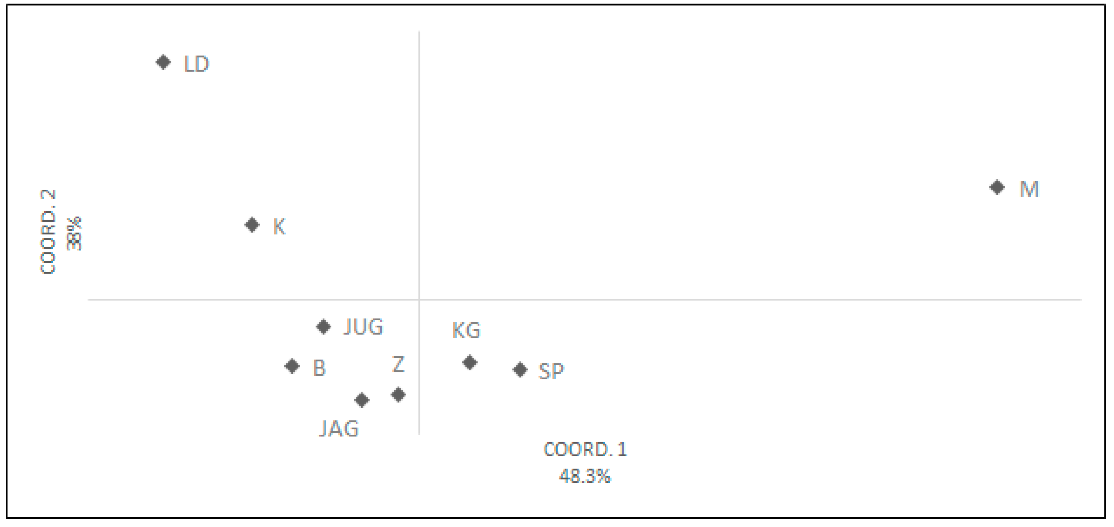
| Trait | First Canonical Variable | Second Canonical Variable |
|---|---|---|
| P | −0.846 *** | 0.355 * |
| E | −0.975 *** | 0.035 |
| A | −0.772 *** | 0.045 |
| B | 0.051 | 0.533 *** |
| Exp | 0.117 | 0.94*** |
| P/E | 0.417 ** | 0.441 ** |
| Exp/P | 0.343 * | 0.873 *** |
| A/B | −0.436 ** | −0.516 *** |
| Percentage variation | 35.27 | 24.50 |
Publisher’s Note: MDPI stays neutral with regard to jurisdictional claims in published maps and institutional affiliations. |
© 2020 by the authors. Licensee MDPI, Basel, Switzerland. This article is an open access article distributed under the terms and conditions of the Creative Commons Attribution (CC BY) license (http://creativecommons.org/licenses/by/4.0/).
Share and Cite
Wrońska-Pilarek, D.; Dering, M.; Bocianowski, J.; Lechowicz, K.; Kowalkowski, W.; Barzdajn, W.; Hauke-Kowalska, M. Pollen Morphology and Variability of Abies alba Mill. Genotypes from South-Western Poland. Forests 2020, 11, 1125. https://doi.org/10.3390/f11111125
Wrońska-Pilarek D, Dering M, Bocianowski J, Lechowicz K, Kowalkowski W, Barzdajn W, Hauke-Kowalska M. Pollen Morphology and Variability of Abies alba Mill. Genotypes from South-Western Poland. Forests. 2020; 11(11):1125. https://doi.org/10.3390/f11111125
Chicago/Turabian StyleWrońska-Pilarek, Dorota, Monika Dering, Jan Bocianowski, Kacper Lechowicz, Wojciech Kowalkowski, Władysław Barzdajn, and Maria Hauke-Kowalska. 2020. "Pollen Morphology and Variability of Abies alba Mill. Genotypes from South-Western Poland" Forests 11, no. 11: 1125. https://doi.org/10.3390/f11111125
APA StyleWrońska-Pilarek, D., Dering, M., Bocianowski, J., Lechowicz, K., Kowalkowski, W., Barzdajn, W., & Hauke-Kowalska, M. (2020). Pollen Morphology and Variability of Abies alba Mill. Genotypes from South-Western Poland. Forests, 11(11), 1125. https://doi.org/10.3390/f11111125