Correlation of Field-Measured and Remotely Sensed Plant Water Status as a Tool to Monitor the Risk of Drought-Induced Forest Decline

 , ,
, ,
Abstract
1. Introduction
2. Materials and Methods
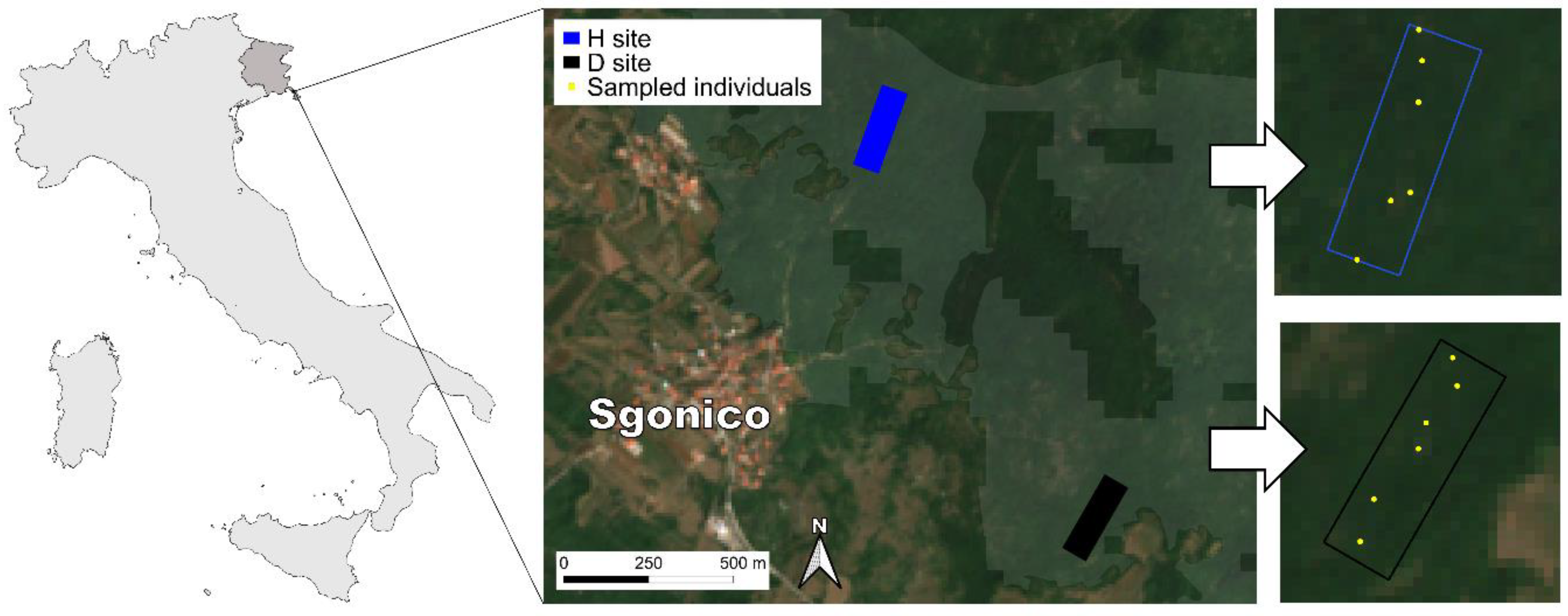
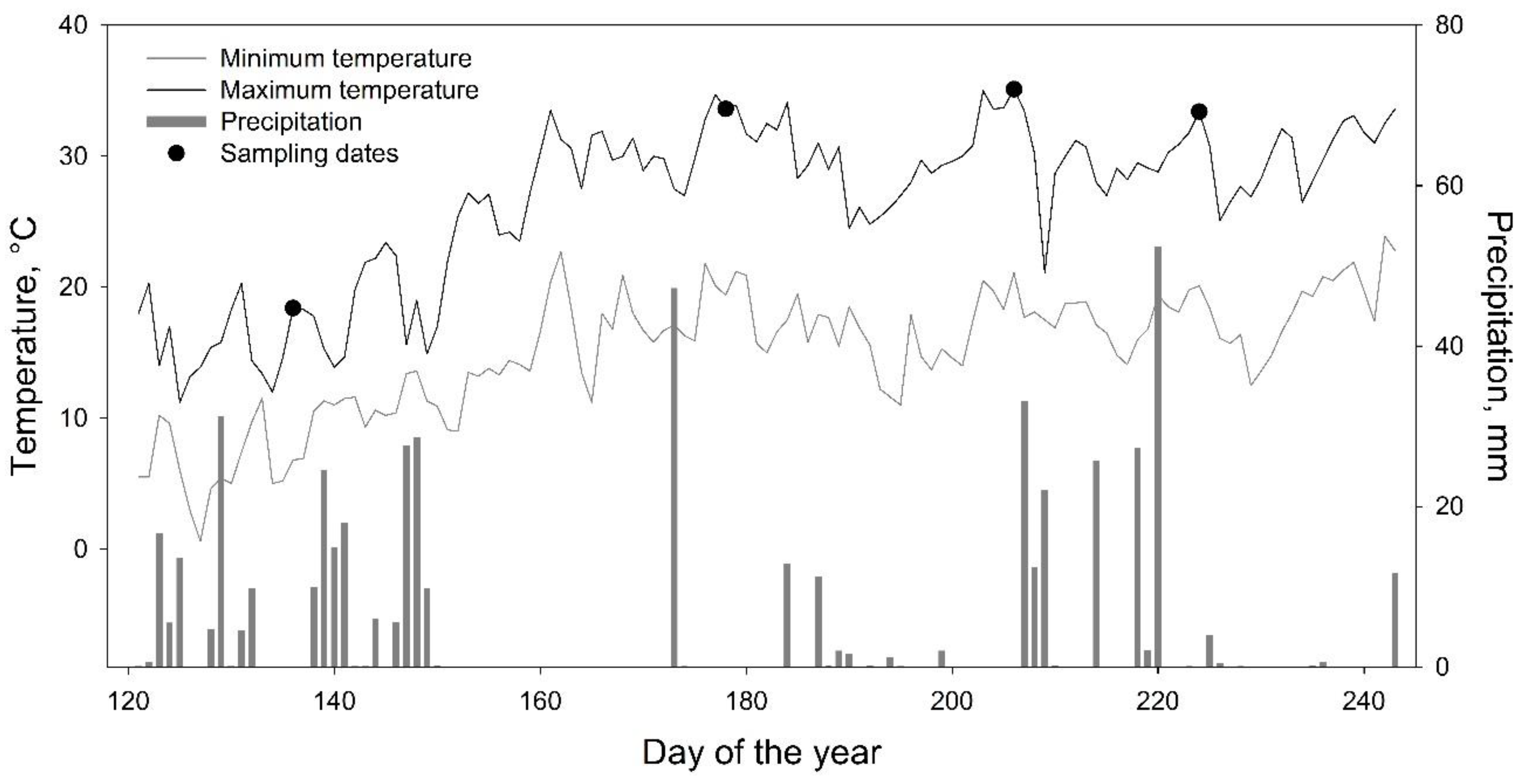
2.1. Study Area
2.2. Physiological Parameters
2.3. Remote Sensing Data
2.4. Statistical Analyses
- Physiological parameter/remote sensing indexsij = Gaussian (μij).
- E(Physiological parameter/remote sensing index) = μij.
- log(Physiological parameter/remote sensing index) = siteij × sampling/acquisition date.
- Sampling/acquisition date ~ N (0, σ2).
3. Results
4. Discussion
5. Conclusions
Author Contributions
Funding
Acknowledgments
Conflicts of Interest
References
- FAO. Global Forest Resources Assessment 2005: Progress towards Sustainable Forest Management; Food and Agriculture Organization of the United Nations: Roma, Italy, 2006; ISBN 978-92-5-105481-9. [Google Scholar]
- Sabine, C.L.; Heimann, M.; Artaxo, P.; Bakker, D.C.E.; Chen, C.T.A.; Field, C.B.; Gruber, N.; Le Quéré, C.; Prinn, R.G.; Richey, J.E.; et al. Current Status and Past Trends of the Global Carbon Cycle. In The Global Carbon Cycle: Integrating Humans, Climate, and the Natural World; Island Press: Washington, DC, USA, 2004; pp. 17–44. ISBN 978-1-55963-527-1. [Google Scholar]
- Allen, C.D.; Macalady, A.K.; Chenchouni, H.; Bachelet, D.; McDowell, N.; Vennetier, M.; Kitzberger, T.; Rigling, A.; Breshears, D.D.; Hogg, E.H.; et al. A global overview of drought and heat-induced tree mortality reveals emerging climate change risks for forests. For. Ecol. Manag. 2010, 259, 660–684. [Google Scholar] [CrossRef]
- Bonan, G.B. Forests and climate change: Forcings, feedbacks, and the climate benefits of forests. Science 2008, 320, 1444–1449. [Google Scholar] [CrossRef] [PubMed]
- Peñuelas, J.; Lloret, F.; Montoya, R. Severe drought effects on Mediterranean woody flora in Spain. For. Sci. 2001, 47, 214–218. [Google Scholar]
- Bréda, N.; Huc, R.; Granier, A.; Dreyer, E. Temperate forest trees and stands under severe drought: A review of ecophysiological responses, adaptation processes and long-term consequences. Ann. For. Sci. 2006, 63, 625–644. [Google Scholar] [CrossRef]
- Bigler, C.; Gavin, D.G.; Gunning, C.; Veblen, T.T. Drought induces lagged tree mortality in a subalpine forest in the Rocky Mountains. Oikos 2007, 116, 1983–1994. [Google Scholar] [CrossRef]
- Lloyd, A.H.; Bunn, A.G. Responses of the circumpolar boreal forest to 20th century climate variability. Environ. Res. Lett. 2007, 2, 045013. [Google Scholar] [CrossRef]
- Van Mantgem, P.J.; Stephenson, N.L. Apparent climatically induced increase of tree mortality rates in a temperate forest. Ecol. Lett. 2007, 10, 909–916. [Google Scholar] [CrossRef]
- Van Mantgem, P.J.; Stephenson, N.L.; Byrne, J.C.; Daniels, L.D.; Franklin, J.F.; Fulé, P.Z.; Harmon, M.E.; Larson, A.J.; Smith, J.M.; Taylor, A.H.; et al. Widespread Increase of Tree Mortality Rates in the Western United States. Science 2009, 323, 521–524. [Google Scholar] [CrossRef]
- Stocker, T.F.; Qin, D.; Plattner, G.K.; Tignor, M.; Allen, S.K.; Boschung, J.; Nauels, A.; Xia, Y.; Bex, V.; Midgley, P.M. Climate Change 2013: The Physical Science Basis; Cambridge University Press: Cambridge, UK, 2013. [Google Scholar]
- Choat, B.; Jansen, S.; Brodribb, T.J.; Cochard, H.; Delzon, S.; Bhaskar, R.; Bucci, S.J.; Feild, T.S.; Gleason, S.M.; Hacke, U.G.; et al. Global convergence in the vulnerability of forests to drought. Nature 2012, 491, 752–755. [Google Scholar] [CrossRef]
- McMahon, S.M.; Arellano, G.; Davies, S.J. The importance and challenges of detecting changes in forest mortality rates. Ecosphere 2019, 10, e02615. [Google Scholar] [CrossRef]
- McDowell, N.G.; Fisher, R.A.; Xu, C.; Domec, J.C.; Hölttä, T.; Mackay, D.S.; Sperry, J.S.; Boutz, A.; Dickman, L.; Gehres, N.; et al. Evaluating theories of drought-induced vegetation mortality using a multimodel–experiment framework. New Phytol. 2013, 304–321. [Google Scholar] [CrossRef] [PubMed]
- Anderegg, W.R.L.; Flint, A.; Huang, C.; Flint, L.; Berry, J.A.; Davis, F.W.; Sperry, J.S.; Field, C.B. Tree mortality predicted from drought-induced vascular damage. Nat. Geosci. 2015, 8, 367–371. [Google Scholar] [CrossRef]
- McDowell, N.G. Mechanisms linking drought, hydraulics, carbon metabolism, and vegetation mortality. Plant Physiol. 2011, 155, 1051–1059. [Google Scholar] [CrossRef]
- Martinez-Vilalta, J.; Anderegg, W.R.L.; Sapes, G.; Sala, A. Greater focus on water pools may improve our ability to understand and anticipate drought-induced mortality in plants. New Phytol. 2019, 223, 22–32. [Google Scholar] [CrossRef] [PubMed]
- Tyree, M.T.; Sperry, J.S. Vulnerability of xylem to cavitation and embolism. Annu. Rev. Plant Physiol. Plant Mol. Biol. 1989, 40, 19–36. [Google Scholar] [CrossRef]
- Pockman, W.T.; Sperry, J.S.; O’Leary, J.W. Sustained and significant negative water pressure in xylem. Nature 1995, 378, 715–716. [Google Scholar] [CrossRef]
- Weatherley, P.E. Studies in the water relations of the cotton plant. New Phytol. 1950, 49, 81–97. [Google Scholar] [CrossRef]
- Weatherley, P.E. Studies in the water relations of the cotton plant. II. Diurnal and seasonal variations in relative turgidity and environmental factors. New Phytol. 1951, 50, 36–51. [Google Scholar] [CrossRef]
- Sade, N.; Vinocur, B.J.; Diber, A.; Shatil, A.; Ronen, G.; Nissan, H.; Wallach, R.; Karchi, H.; Moshelion, M. Improving plant stress tolerance and yield production: Is the tonoplast aquaporin SlTIP2;2 a key to isohydric to anisohydric conversion? New Phytol. 2009, 181, 651–661. [Google Scholar] [CrossRef]
- Sade, N.; Gebremedhin, A.; Moshelion, M. Risk-taking plants: Anisohydric behavior as a stress-resistance trait. Plant Signal. Behav. 2012, 7, 767–770. [Google Scholar] [CrossRef]
- Anderegg, W.R.L.; Anderegg, L.D.L.; Huang, C. Testing early warning metrics for drought-induced tree physiological stress and mortality. Glob. Chang. Biol. 2019, 25, 2459–2469. [Google Scholar] [CrossRef] [PubMed]
- Rao, K.; Anderegg, W.R.L.; Sala, A.; Martínez-Vilalta, J.; Konings, A.G. Satellite-based vegetation optical depth as an indicator of drought-driven tree mortality. Remote Sens. Environ. 2019, 227, 125–136. [Google Scholar] [CrossRef]
- Sapes, G.; Roskilly, B.; Dobrowski, S.; Maneta, M.; Anderegg, W.R.L.; Martinez-Vilalta, J.; Sala, A. Plant water content integrates hydraulics and carbon depletion to predict drought-induced seedling mortality. Tree Physiol. 2019, 39, 1300–1312. [Google Scholar] [CrossRef]
- Rouse, J.; Haas, R.; Schell, J.; Deering, D. Monitoring vegetation systems in the Great Plains with ERTS. NASA 1974, 1, 309–317. [Google Scholar]
- Tucker, C.J. Red and photographic infrared linear combinations for monitoring vegetation. Remote Sens. Environ. 1979, 8, 127–150. [Google Scholar] [CrossRef]
- Sellers, P.J. Canopy reflectance, photosynthesis and transpiration. Int. J. Remote Sens. 1985, 6, 1335–1372. [Google Scholar] [CrossRef]
- Huete, A.; Didan, K.; Miura, T.; Rodriguez, E.P.; Gao, X.; Ferreira, L.G. Overview of the radiometric and biophysical performance of the MODIS vegetation indices. Remote Sens. Environ. 2002, 83, 195–213. [Google Scholar] [CrossRef]
- Aguilar, C.; Zinnert, J.C.; Polo, M.J.; Young, D.R. NDVI as an indicator for changes in water availability to woody vegetation. Ecol. Indic. 2012, 23, 290–300. [Google Scholar] [CrossRef]
- Frampton, W.J.; Dash, J.; Watmough, G.; Milton, E.J. Evaluating the capabilities of Sentinel-2 for quantitative estimation of biophysical variables in vegetation. Isprs J. Photogramm. Remote Sens. 2013, 82, 83–92. [Google Scholar] [CrossRef]
- Gao, B.; Goetz, A.F.H. Extraction of dry leaf spectral features from reflectance spectra of green vegetation. Remote Sens. Environ. 1994, 47, 369–374. [Google Scholar] [CrossRef]
- Huete, A.R. Soil-dependent spectral response in a developing plant canopy 1. Agron. J. 1987, 79, 61–68. [Google Scholar] [CrossRef]
- Huete, A.R. A soil-adjusted vegetation index (SAVI). Remote Sens. Environ. 1988, 25, 295–309. [Google Scholar] [CrossRef]
- Gao, B. NDWI—A normalized difference water index for remote sensing of vegetation liquid water from space. Remote Sens. Environ. 1996, 58, 257–266. [Google Scholar] [CrossRef]
- Wang, C.; Lu, Z.; Haithcoat, T.L. Using Landsat images to detect oak decline in the Mark Twain National Forest, Ozark Highlands. For. Ecol. Manag. 2007, 240, 70–78. [Google Scholar] [CrossRef]
- Majasalmi, T.; Rautiainen, M. The potential of Sentinel-2 data for estimating biophysical variables in a boreal forest: A simulation study. Remote Sens. Lett. 2016, 7, 427–436. [Google Scholar] [CrossRef]
- Urban, M.; Berger, C.; Mudau, T.E.; Heckel, K.; Truckenbrodt, J.; Onyango Odipo, V.; Smit, I.P.J.; Schmullius, C. Surface moisture and vegetation cover analysis for drought monitoring in the Southern Kruger National Park using Sentinel-1, Sentinel-2, and Landsat-8. Remote Sens. 2018, 10, 1482. [Google Scholar] [CrossRef]
- Bowman, W.D. The relationship between leaf water status, gas exchange, and spectral reflectance in cotton leaves. Remote Sens. Environ. 1989, 30, 249–255. [Google Scholar] [CrossRef]
- Ben-Gal, A.; Agam, N.; Alchanatis, V.; Cohen, Y.; Yermiyahu, U.; Zipori, I.; Presnov, E.; Sprintsin, M.; Dag, A. Evaluating water stress in irrigated olives: Correlation of soil water status, tree water status, and thermal imagery. Irrig. Sci. 2009, 27, 367–376. [Google Scholar] [CrossRef]
- Berni, J.A.J.; Zarco-Tejada, P.J.; Sepulcre-Cantó, G.; Fereres, E.; Villalobos, F. Mapping canopy conductance and CWSI in olive orchards using high resolution thermal remote sensing imagery. Remote Sens. Environ. 2009, 113, 2380–2388. [Google Scholar] [CrossRef]
- Krishna, G.; Sahoo, R.N.; Singh, P.; Patra, H.; Bajpai, V.; Das, B.; Kumar, S.; Dhandapani, R.; Vishwakarma, C.; Pal, M.; et al. Application of thermal imaging and hyperspectral remote sensing for crop water deficit stress monitoring. Geocarto Int. 2019, 1–14. [Google Scholar] [CrossRef]
- Sun, H.; Feng, M.; Xiao, L.; Yang, W.; Wang, C.; Jia, X.; Zhao, Y.; Zhao, C.; Muhammad, S.K.; Li, D. Assessment of plant water status in winter wheat (Triticum aestivum L.) based on canopy spectral indices. PLoS ONE 2019, 14, e0216890. [Google Scholar] [CrossRef] [PubMed]
- Petrucco, L.; Nardini, A.; von Arx, G.; Saurer, M.; Cherubini, P. Isotope signals and anatomical features in tree rings suggest a role for hydraulic strategies in diffuse drought-induced die-back of Pinus nigra. Tree Physiol. 2017, 37, 523–535. [Google Scholar] [PubMed]
- GRASS Development Team Geographic Resources Analysis Support System (GRASS); Software, Version 7.2; Open Source Geospatial Foundation: Chicago, IL, USA, 2017.
- Nardini, A.; Battistuzzo, M.; Savi, T. Shoot desiccation and hydraulic failure in temperate woody angiosperms during an extreme summer drought. New Phytol. 2013, 200, 322–329. [Google Scholar] [CrossRef] [PubMed]
- Nardini, A.; Salleo, S.; Trifilò, P.; Lo Gullo, M.A. Water relations and hydraulic characteristics of three woody species co-occurring in the same habitat. Ann. For. Sci. 2003, 60, 297–305. [Google Scholar] [CrossRef]
- Tomasella, M.; Casolo, V.; Aichner, N.; Petruzzellis, F.; Savi, T.; Trifilò, P.; Nardini, A. Non-structural carbohydrate and hydraulic dynamics during drought and recovery in Fraxinus ornus and Ostrya carpinifolia saplings. Plant Physiol. Biochem. 2019, 145, 1–9. [Google Scholar] [CrossRef]
- QGIS Development Team QGIS Geographic Information System; Open Source Geospatial Foundation Project, Versão, Version 2.7. Available online: https://qgis.org/it/site/ (accessed on 8 January 2020).
- Drusch, M.; Del Bello, U.; Carlier, S.; Colin, O.; Fernandez, V.; Gascon, F.; Hoersch, B.; Isola, C.; Laberinti, P.; Martimort, P.; et al. Sentinel-2: ESA’s Optical High-Resolution Mission for GMES Operational Services. Remote Sens. Environ. 2012, 120, 25–36. [Google Scholar] [CrossRef]
- ESA Sentinel-2. Available online: https://sentinel.esa.int/web/sentinel/missions/sentinel-2/heritage (accessed on 8 January 2020).
- R Core Team. R: A Language and Environment for Statistical Computing; R Foundation for Statistical Computing; CRAN: Vienna, Austria, 2019. [Google Scholar]
- Bates, D.; Mächler, M.; Bolker, B.; Walker, S. Fitting linear mixed-effects models using lme4. J. Stat. Softw. 2015, 67, 1–48. [Google Scholar] [CrossRef]
- Barton, K.; Barton, M.K. Multi-Model Inference; CRAN: Vienna, Austria, 2019. [Google Scholar]
- Dennison, P.E.; Roberts, D.A.; Peterson, S.H.; Rechel, J. Use of Normalized Difference Water Index for monitoring live fuel moisture. Int. J. Remote Sens. 2005, 26, 1035–1042. [Google Scholar] [CrossRef]
- Carter, G.A. Primary and Secondary Effects of water content on the spectral reflectance of leaves. Am. J. Bot. 1991, 78, 916–924. [Google Scholar] [CrossRef]
- Aldakheel, Y.Y.; Danson, F.M. Spectral reflectance of dehydrating leaves: Measurements and modelling. Int. J. Remote Sens. 1997, 18, 3683–3690. [Google Scholar] [CrossRef]
- Maki, M.; Ishiahra, M.; Tamura, M. Estimation of leaf water status to monitor the risk of forest fires by using remotely sensed data. Remote Sens. Environ. 2004, 90, 441–450. [Google Scholar] [CrossRef]


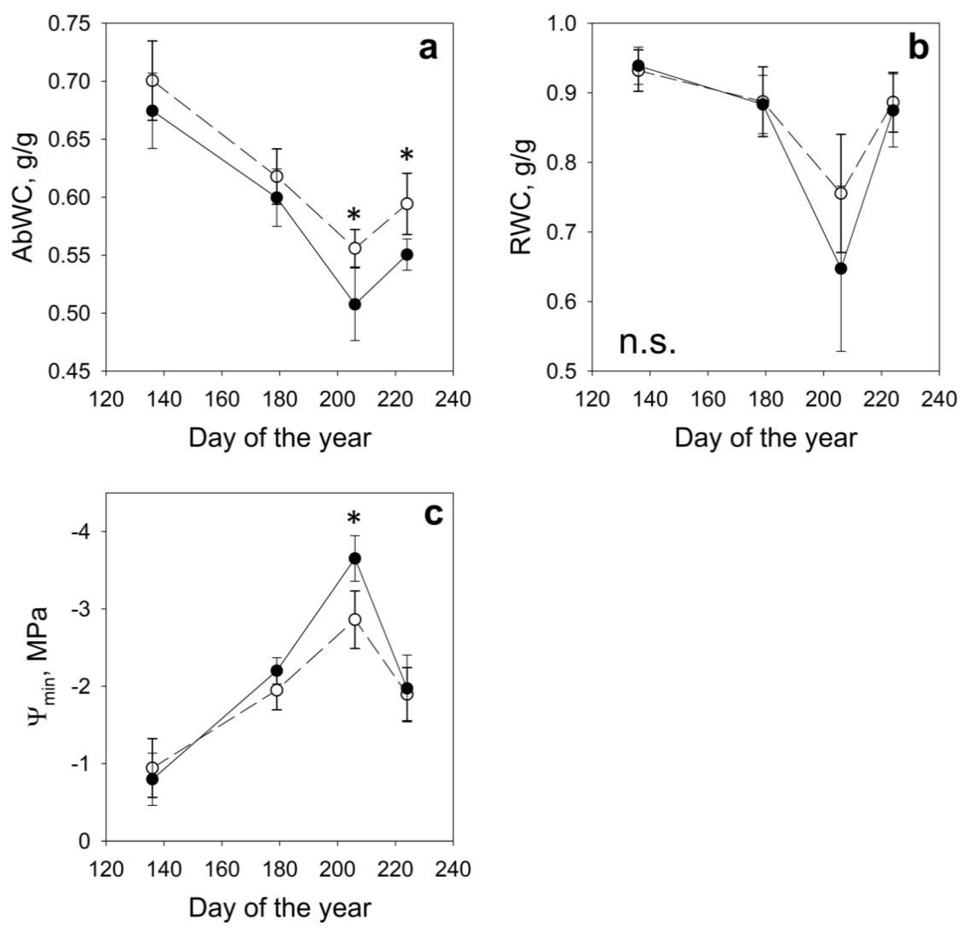
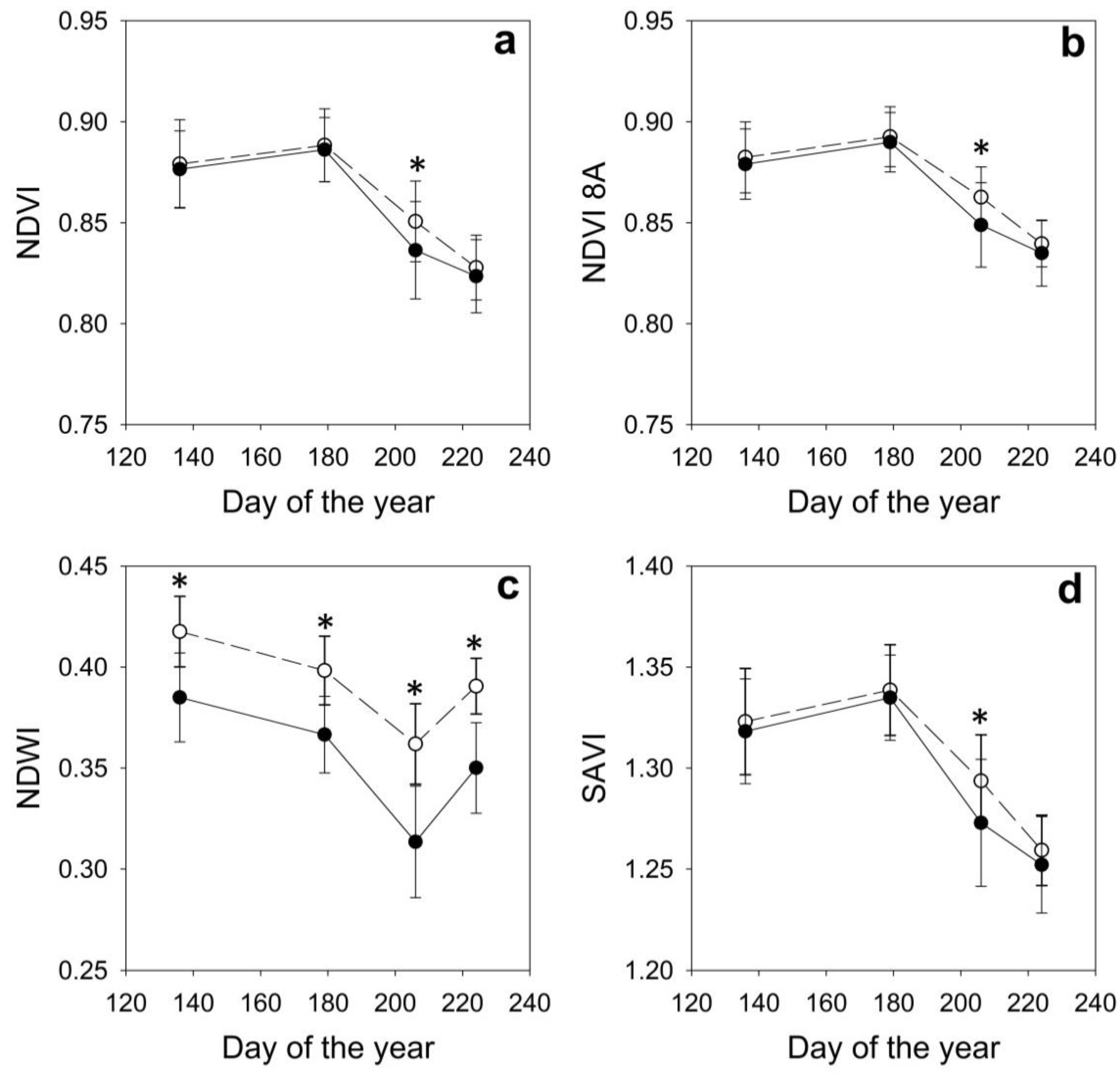
| DOY | Date | Site | AbWc g/g | RWC g/g | Ψmin MPa | NDVI | NDVI 8A | NDWI | SAVI |
|---|---|---|---|---|---|---|---|---|---|
| 136 | May 16th | H | 0.70 ± 0.03 | 0.93 ± 0.03 | −0.94 ± 0.38 | 0.886 ± 0.012 | 0.889 ± 0.011 | 0.428 ± 0.016 | 1.333 ± 0.016 |
| D | 0.67 ± 0.03 | 0.94 ± 0.03 | −0.80 ± 0.34 | 0.870 ± 0.021 | 0.873 ± 0.020 | 0.380 ± 0.026 | 1.309 ± 0.029 | ||
| 179 | June 28th | H | 0.62 ± 0.02 | 0.89 ± 0.05 | −1.95 ± 0.25 | 0.902 ± 0.013 | 0.905 ± 0.011 | 0.410 ± 0.013 | 1.358 ± 0.017 |
| D | 0.60 ± 0.02 | 0.89 ± 0.04 | −2.20 ± 0.17 | 0.880 ± 0.016 | 0.884 ± 0.014 | 0.359 ± 0.022 | 1.326 ± 0.022 | ||
| 206 | July 25th | H | 0.56 ± 0.02 | 0.76 ± 0.08 | −2.86 ± 0.37 | 0.859 ± 0.013 | 0.870 ± 0.011 | 0.362 ± 0.018 | 1.305 ± 0.016 |
| D | 0.51 ± 0.03 | 0.65 ± 0.12 | −3.65 ± 0.29 | 0.826 ± 0.027 | 0.839 ± 0.024 | 0.308 ± 0.031 | 1.259 ± 0.036 | ||
| 224 | August 12th | H | 0.59 ± 0.03 | 0.89 ± 0.04 | −1.90 ± 0.34 | 0.837 ± 0.013 | 0.848 ± 0.011 | 0.392 ± 0.019 | 1.272 ± 0.016 |
| D | 0.55 ± 0.01 | 0.87 ± 0.05 | −1.97 ± 0.43 | 0.816 ± 0.017 | 0.827 ± 0.015 | 0.353 ± 0.022 | 1.241 ± 0.022 |
| NDVI | NDVI 8A | NDWI | SAVI | ||
|---|---|---|---|---|---|
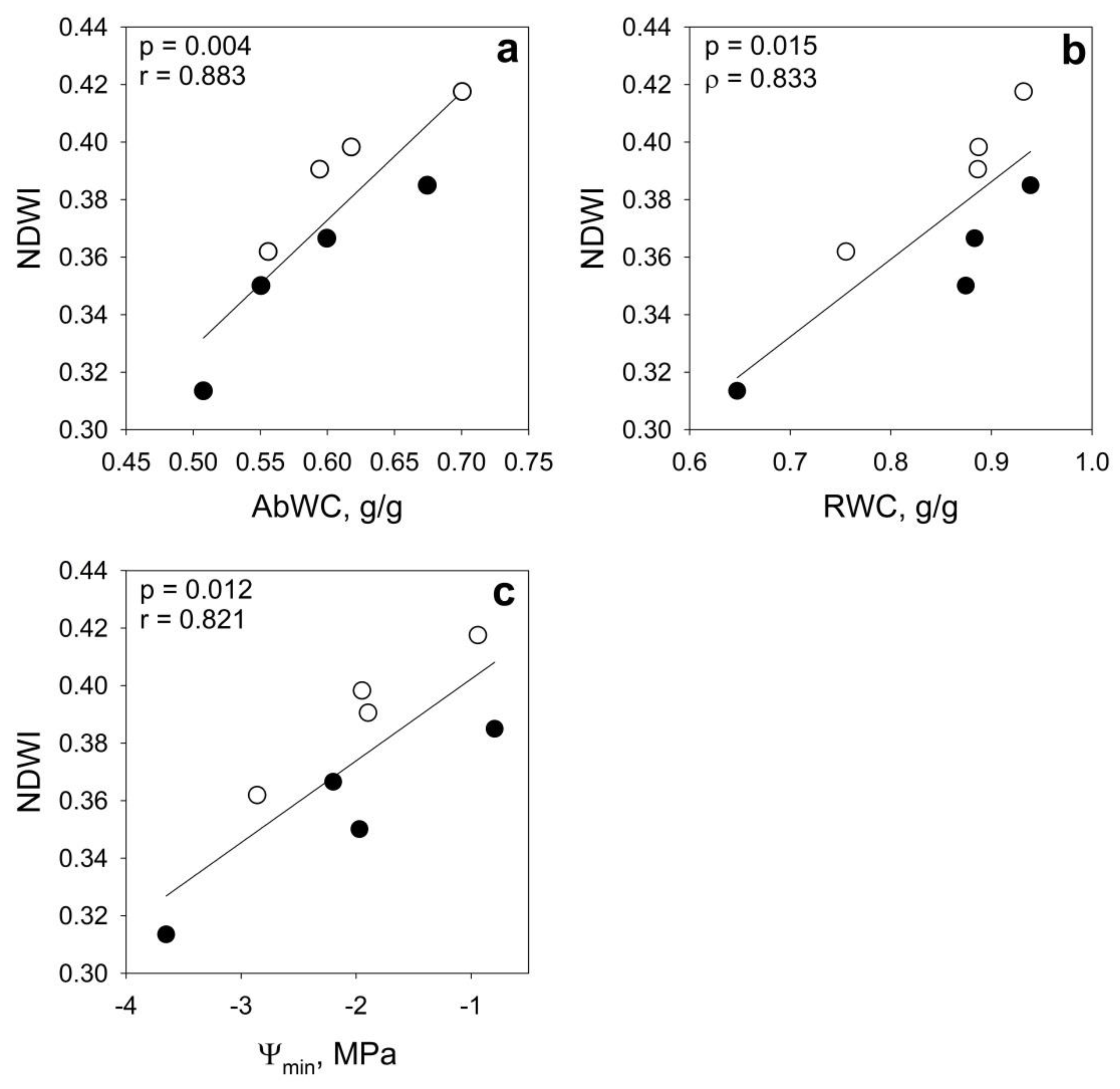
| AbWC | r | 0.676 | 0.630 | 0.883 ** | 0.628 |
| RWC | ρ | 0.476 | 0.476 | 0.833 * | 0.476 |
| Ψmin | r | 0.446 | 0.382 | 0.821 * | 0.381 |
© 2020 by the authors. Licensee MDPI, Basel, Switzerland. This article is an open access article distributed under the terms and conditions of the Creative Commons Attribution (CC BY) license (http://creativecommons.org/licenses/by/4.0/).
Share and Cite
Marusig, D.; Petruzzellis, F.; Tomasella, M.; Napolitano, R.; Altobelli, A.; Nardini, A. Correlation of Field-Measured and Remotely Sensed Plant Water Status as a Tool to Monitor the Risk of Drought-Induced Forest Decline. Forests 2020, 11, 77. https://doi.org/10.3390/f11010077
Marusig D, Petruzzellis F, Tomasella M, Napolitano R, Altobelli A, Nardini A. Correlation of Field-Measured and Remotely Sensed Plant Water Status as a Tool to Monitor the Risk of Drought-Induced Forest Decline. Forests. 2020; 11(1):77. https://doi.org/10.3390/f11010077
Chicago/Turabian StyleMarusig, Daniel, Francesco Petruzzellis, Martina Tomasella, Rossella Napolitano, Alfredo Altobelli, and Andrea Nardini. 2020. "Correlation of Field-Measured and Remotely Sensed Plant Water Status as a Tool to Monitor the Risk of Drought-Induced Forest Decline" Forests 11, no. 1: 77. https://doi.org/10.3390/f11010077
APA StyleMarusig, D., Petruzzellis, F., Tomasella, M., Napolitano, R., Altobelli, A., & Nardini, A. (2020). Correlation of Field-Measured and Remotely Sensed Plant Water Status as a Tool to Monitor the Risk of Drought-Induced Forest Decline. Forests, 11(1), 77. https://doi.org/10.3390/f11010077