Article

Object-Based Tree Species Classification Using Airborne Hyperspectral Images and LiDAR Data

1
Beijing Key Laboratory of Precision Forestry, Forestry College, Beijing Forestry University, Beijing 100083, China
2
Key Laboratory for Forest Silviculture and Conservation of the Ministry of Education, Beijing Forestry University, Beijing 100083, China
3
Heilongjiang Institute of Geomatics Engineering, Harbin 150081, China
*
Author to whom correspondence should be addressed.
Forests 2020, 11(1), 32; https://doi.org/10.3390/f11010032
Submission received: 10 November 2019 / Revised: 19 December 2019 / Accepted: 21 December 2019 / Published: 24 December 2019

Abstract

:
The identification of tree species is one of the most basic and key indicators in forest resource monitoring with great significance in the actual forest resource survey and it can comprehensively improve the efficiency of forest resource monitoring. The related research has mainly focused on single tree species without considering multiple tree species, and therefore the ability to classify forest tree species in complex stand is not clear, especially in the subtropical monsoon climate region of southern China. This study combined airborne hyperspectral data with simultaneously acquired LiDAR data, to evaluate the capability of feature combinations and k-nearest neighbor (KNN) and support vector machine (SVM) classifiers to identify tree species, in southern China. First, the stratified classification method was used to remove non-forest land. Second, the feature variables were extracted from airborne hyperspectral image and LiDAR data, including independent component analysis (ICA) transformation images, spectral indices, texture features, and canopy height model (CHM). Third, random forest and recursion feature elimination methods were adopted for feature selection. Finally, we selected different feature combinations and used KNN and SVM classifiers to classify tree species. The results showed that the SVM classifier has a higher classification accuracy as compared with KNN classifier, with the highest classification accuracy of 94.68% and a Kappa coefficient of 0.937. Through feature elimination, the classification accuracy and performance of SVM classifier was further improved. Recursive feature elimination method based on SVM is better than random forest. In the spectral indices, the new constructed slope spectral index, SL2, has a certain effect on improving the classification accuracy of tree species. Texture features and CHM height information can effectively distinguish tree species with similar spectral features. The height information plays an important role in improving the classification accuracy of other broad-leaved species. In general, the combination of different features can improve the classification accuracy, and the proposed strategies and methods are effective for the identification of tree species at complex forest type in southern China.

1. Introduction

As a renewable resource, forest plays an important role in the survival and development of human civilization [1]. A timely understanding of the stock and distribution of forest resources is the basis for the sustainable development of forestry [2]. Nowadays, tree species classification of complex forests is becoming a very important research direction. However, with the changing climatic conditions and the interference of natural and human factors, the richness of forest species has been decreasing [3], which has seriously affected the sustainable development of the forests [4]. In addition, the accuracy of the estimation of forest on-ground carbon stocks is also dependent on the accuracy of tree species identification [5,6]. In the past, tree species were mainly identified with fieldwork, which was time consuming, laborious, and costly. With the rapid development of remote sensing technology, remote sensing image data plays an important role in forestry species identification [7,8].
At present, wide-spectrum, medium- and low-resolution remote sensing data are widely used [9,10]. Because of the low spatial and spectral resolution, only forest types can be identified. Hyperspectral imagery contains near-continuous spectral information of the ground object, which can accurately detect different objects with fine spectral differences, and therefore the recognition accuracy of tree species is improved for the source data [11,12,13]. Zhang et al. [14] used wavelet transform to process HYDICE hyperspectral data and identify tree species in tropical forests and found that hyperspectral data after wavelet transform can improve the recognition accuracy. Dian et al. [15] used airborne hyperspectral images for forest tree species classification, which proved that combining the spatial and spectral information can improve the accuracy of tree species classification. Fagan et al. [16] used hyperspectral and multitemporal Landsat imagery to classify forest and tree plantations in northeastern Costa Rica. The results indicated that using hyperspectral data alone classified six species of tree plantations with 75% to 93% producer’s accuracy, however, for fine classification of tree species, the effectiveness of classification is still limited only by hyperspectral images.
The classification of remote sensing images is mainly based on pixels or objects. Classifiers based on pixels has been widely used over the past decades [17,18], and the object-based method for tree species identification has recently emerged, which is proposed for the development of high spatial resolution data [19,20,21]. The key technology of object-based classification is image segmentation. The segmentation quality and precision depend on the classification algorithms and how to perform optimal scale segmentation qualitatively or quantitatively [22,23]. Immitzer et al. [24] found that the object-based method is better than the pixel-based method when using very high spatial resolution data. Wang et al. [25] combined decision tree method (DT) with the object-based method to carry out vegetation research in the Yushu area which overcame the “salt and pepper” and improved the classification accuracy effectively.
Because the distribution of ground objects has a certain continuity, there is a correlation between adjacent pixels on the remote sensing image. Hyperspectral can only characterize the horizontal direction of the forest, which makes the phenomenon of different objects having the same spectrum and the same objects having different spectrum [24]. Therefore, even with spectral images of high spatial resolution, it is difficult to classify all tree species. As an important supplementary feature, spatial structure information makes it possible to classify tree species at a finer scale [26,27]. Airborne LiDAR data can characterize the vertical structure information of the stand, which has obvious advantages for forest type identification and forest structure characteristics [12,28]. Hollaus et al. [29] used LiDAR data to extract the canopy height of single trees. The results showed that the correlation between LiDAR tree height and field tree height was very good. Heinzel et al. [30] used high density full-waveform LiDAR data for tree species classification and found that up to six tree species were classified with an overall accuracy of 57%. Since airborne LiDAR can only obtain the three-dimensional information of the vertical structure of the tree species, it is less able to improve the related information of the tree species in horizontal direction [31]. However, the type of single wood cannot be accurately determined based on tree height or crown information, therefore, in tree species identification, airborne LiDAR data needs to be combined with hyperspectral data to take the advantage of it.
Therefore, the combination of hyperspectral imagery with LiDAR data to achieve complementary advantages and application in forestry has become a new research hotspot. Some scholars have carried out related studies in this field [32,33]. Voss et al. [34] combined multitemporal AISA hyperspectral data with LiDAR data and used object-oriented classification methods for tree species classification in an urban environment; the final classification accuracy is higher than the accuracy of a single data source classification. Liu et al. [35] used support vector machine (SVM) classifier to identify complex forest species in northern China based on airborne LiDAR and hyperspectral data fusion and found that the classification accuracy of the fused data was higher than using spectral data alone, and the overall accuracy reached 83.88%, and the Kappa coefficient was 0.80. Cao et al. [36] used unmanned aerial vehicle (UAV) hyperspectral images and digital surface model (DSM) to classify mangrove species. The results showed that height information played an important role in improving the classification accuracy.
Considering the advantages of airborne hyperspectral imagery and LiDAR point cloud in structure, the combination of the two data was applied to the recognition and classification of ground objects. Related studies have mainly focused on single tree species without considering multiple tree species, and therefore the ability to classify tree species in complex forest type is not clear, especially in the subtropical monsoon climate region of southern China. Therefore, the main objectives of this study include the following: To combine hyperspectral images with simultaneously acquired LiDAR data, using different combinations of features and classifiers for object-based classification; to evaluate the capability of airborne hyperspectral and LiDAR data for accurate identification of tree species in complex forest stand in the subtropical monsoon climate region of southern China; and also to compare and analyze the contributions of different feature variables and classifiers.

2. Materials and Methods
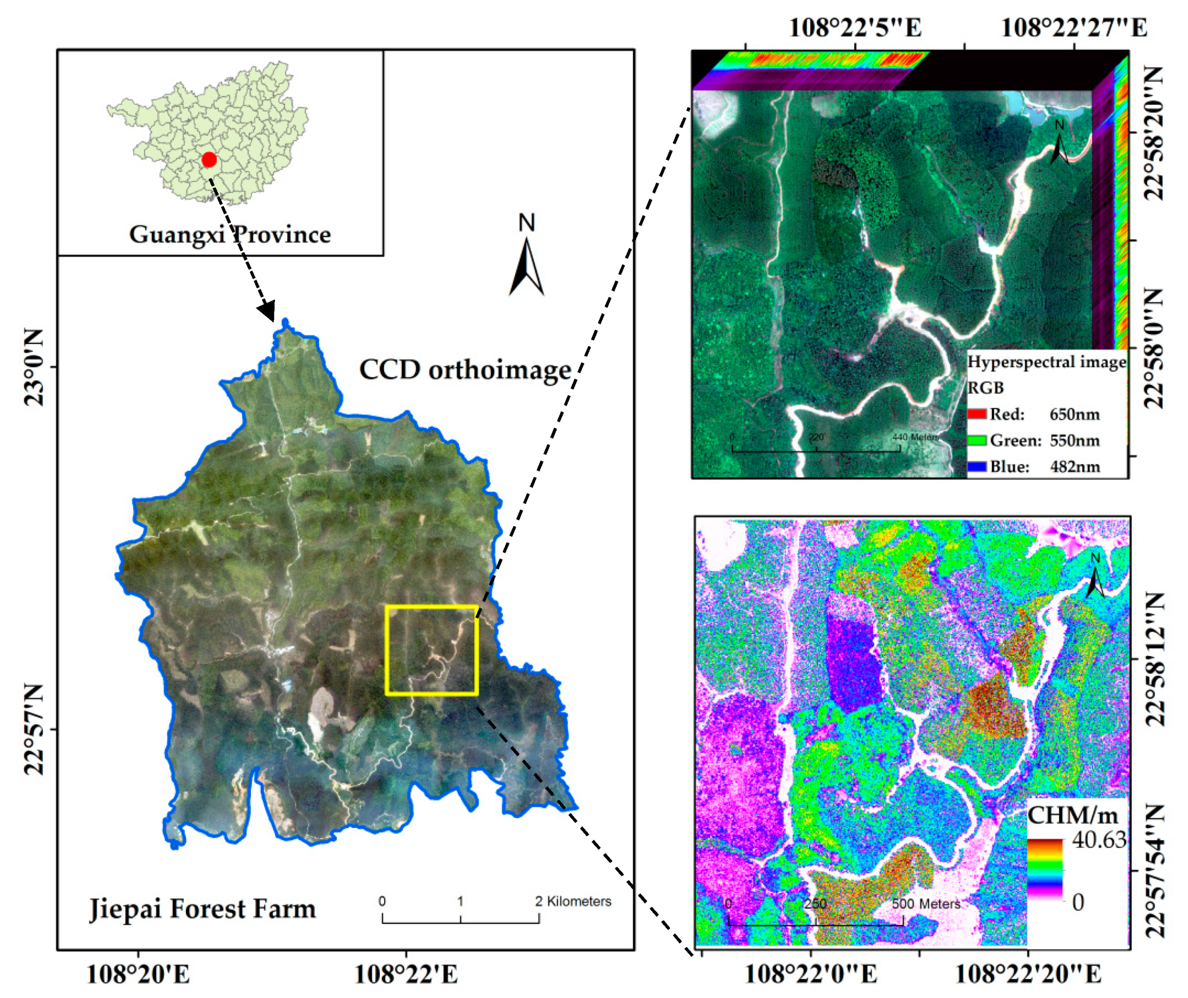
2.1. Study Area

This study was carried out in Jiepai Forest Farm in Gaofeng Forest Farm of Nanning City, Guangxi Province, China (22°56′41″–23°0′21″ N, 108°19′47″–109°23′16″ E), as shown in Figure 1. The area is a hilly landform, the altitude is 100 to 300 m, and the slope is 6 to 35° [37]. It belongs to the south subtropical monsoon climate, with abundant sunshine and rainfall. The annual average temperature is about 21 °C, rainfall is 1200 to 1500 mm, and the annual evaporation is 1250 to 1620 mm [38], which is suitable for the growth of tropical and subtropical tree species. The forest type has typical characteristics of southern China forest [39]. For the study site, we chose an area with abundant tree species, covering an area of 128 ha (as the yellow polygon in Figure 1). The tree species mainly include Chinese fir (Cunninghamia lanceolata (Lamb.) Hook.), eucalyptus (Eucalyptus robusta Smith), Illicium verum (Illicium verum Hook.f.), mytilaria laosensis (Mytilaria laosensis Lec.), slash pine (Pinus elliottii Engelm.), and masson pine (Pinus massoniana Lamb.). At the study site, the broad-leaved species are varied and the samples are limited, and therefore they are not subdivided into tree species, but rather called other broad leaves. In addition, some forest land for seedling storage and cutting sites were collectively referred to as other forest land, and non-forest land was divided into water, road, and buildings. Table 1 is the specific classification system of the study area.

2.2. Data Collection and Preprocessing

2.2.1. Data Collection

Datasets used in this study were acquired by the CAF’s (the Chinese Academy of Forestry) LiCHy (LiDAR, CCD, and Hyperspectral) Airborne Observation System [40], which collects hyperspectral images, LiDAR data, and CCD images synchronously. Hyperspectral images were collected using an AISA Eagle II (Spectral Imaging Ltd., Oulu, Finland) hyperspectral sensor for LiCHy system [41]. It is a push broom imaging system and covers the VNIR spectral ranges from 400 nm to 1000 nm. The RIEGL LMS-Q680i with a full waveform LiDAR system was carried as the laser sensor [42] and provided high-precision digital elevation model (DEM) and digital surface model (DSM). A medium-format airborne digital camera system (DigiCAM-60) was selected as the CCD sensor [43] with 0.2 m spatial resolution. The data was collected on 13 January and 30 January 2018 at Jiepai Forest Farm in Nanning, Guangxi province. The actual flight altitude was approximately 1000 m, and the data acquisition day was sunny and cloudless. Detailed parameters of the three earth observation sensors are shown in Table 2.
At the same time, the field survey was carried out from 16 January 2018 to 5 February 2018, mainly in the pure Chinese fir forest, pure eucalyptus forest, and other mixed forests. A total of 19 plots were investigated in the study area, of which 6 plots are pure eucalyptus forest, 7 plots are pure Chinese fir forest, and the rest are other mixed forests, a total of 1657 trees. The tree species includes eucalyptus, Chinese fir, Illicium verum, masson pine, etc. The plots are 25 × 25 m in size, recorded data include the location, plot number, aspect, tree species, tree height, tree crown width, and other basic measurement factors. During the field work, we collected some sampling points and recorded the precise location using a handheld GPS device, including latitude and longitude and tree species information. The positioning accuracy of sampling points is available, which can be used for extraction of training and validation samples. Additional reference data included subcompartment data. The main reference factors included types of ground objects and dominant tree species information, which were used as reference for vegetation cover types and tree species distribution in the forest farm.

2.2.2. Data Preprocessing

The airborne hyperspectral data have been preprocessed by the data providers including radiometric calibration, geometric correction, and orthorectification, as well as we processed data for mosaicing and cropping, atmospheric correction, denoising, and geometric registration with LiDAR data. Because the flight altitude was relatively low, the hyperspectral data was less affected by the atmosphere, thus it facilitated to correction. In this study we used MODTRAN 4+ radiation transfer model [44] supported by ENVI to perform atmospheric correction on hyperspectral data, which can correct the cascade effect caused by diffuse reflection and adjust the spectrum smoothing caused by artificial suppression. The minimum noise fraction rotation (MNF) method was used to remove image noise with its advantage for hyperspectral data denoising.
According to the field survey data and CCD orthoimages, we selected typical tree species samples of above seven tree species and extracted the mean spectral reflectance curves (Figure 2). The vegetation spectral curve highlights the valley and peak, and the near-infrared bands form a distinct high reflection peak, which is consistent with the spectral curve characteristics of the vegetation. Comparing the spectral reflectance of each tree species, there is greater separability in the near-infrared spectral region, and the spectral reflectance values of broad-leaved species are generally higher than conifer species.
The LiDAR data provided more control to users for vertical information analysis. The horizontal accuracy of LiDAR is about 0.5 m and the vertical accuracy is about 0.3 m after comparing with typical observation targets. The consistency of LiDAR and CCD products is within 1 pixel for gentle slope areas and 1 to 2 pixels for hilly areas. The canopy height model (CHM) extracted from airborne LiDAR data is an important feature variable. The processing mainly contains filtering classification to separate ground and non-ground points from the point cloud data. Before classifying ground points, abnormal points should be filtered out, including points that are significantly lower than the ground or higher than the surface target, and moving object points. A digital elevation model (DEM) was created by performing a triangulated irregular network (TIN) [45] interpolation operation using the point cloud product that was already separated as ground points. Meanwhile, the digital surface model (DSM) was generated by interpolating the first return points. The CHM elevation-normalized data were obtained by conducting a grid difference calculation between DSM and DEM [35].
The hyperspectral data and the LiDAR CHM data should perform coregistration. We used the nearest neighbor resampling method [46] and selected 20 representative control points on the two images for coregistration, which were located along the road or flat area. The average error of the control points was less than one pixel. Thus, the coregistration result of the two data was confidential.

2.3. Sample Collection

According to the field survey data and the position of the tree species recorded in the field observation, combining with the high spatial resolution CCD orthoimages and subcompartment data, we randomly chose 522 image-object samples in the study site for training, each image-object sample covered several complete canopies, which ensured the training sample was more representative. We selected 372 image-object samples for validating the results. These samples were evenly distributed throughout the study site, ensuring that training samples and validation samples were not duplicated. Table 3 shows the number of training samples and verification samples for each tree species.

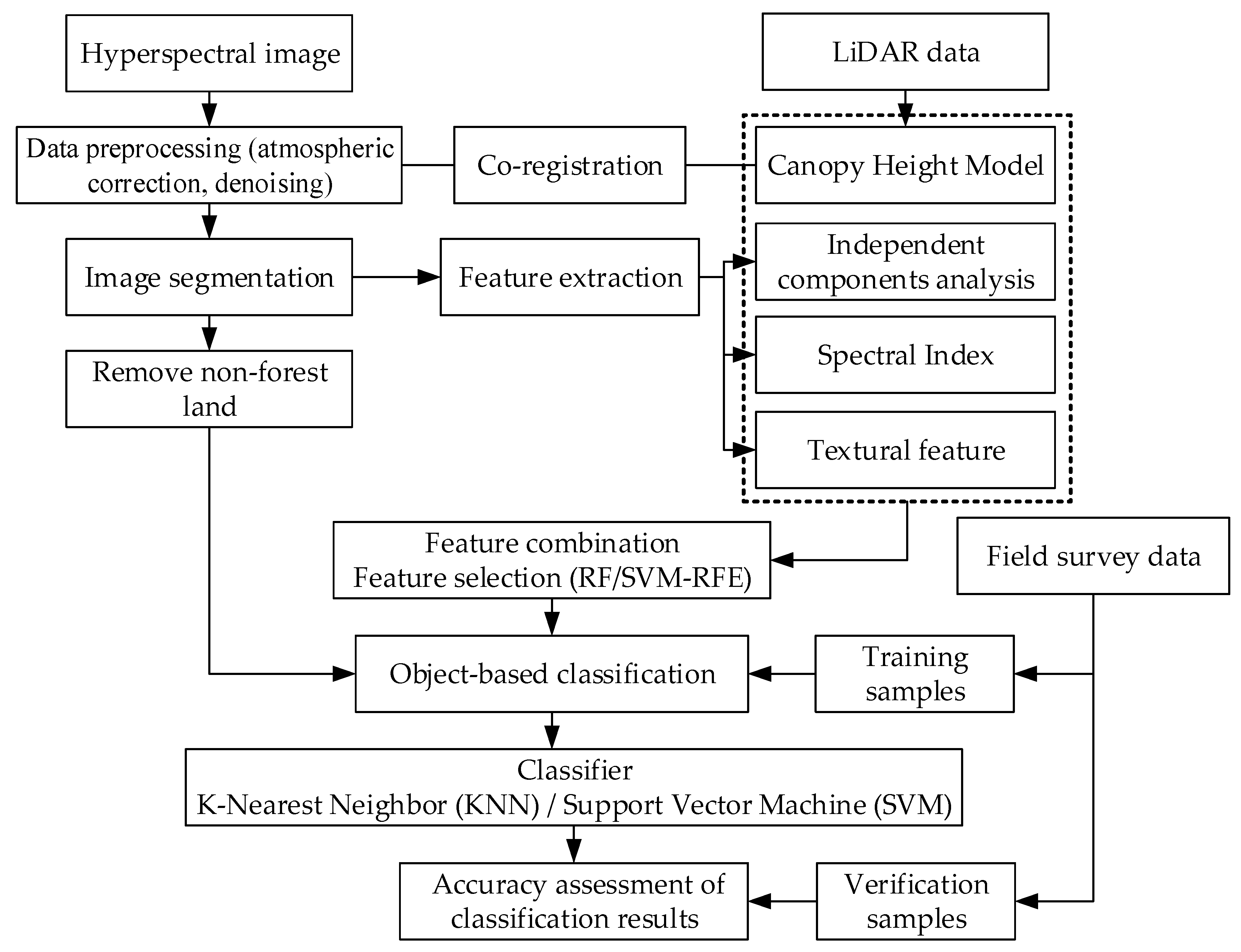
2.4. Workflow Description

The workflow of this study is illustrated in Figure 3. We used airborne hyperspectral images and LiDAR data for object-based tree species classification. The classification process includes five major steps: (1) Stratified classification is used to remove non-forest land and avoid confusion with tree species; (2) extraction of feature variables from airborne hyperspectral image and LiDAR data and using random forest and recursive feature elimination method for selecting the optimal combination of feature variables; (3) selection of the optimal segmentation parameters for image segmentation; (4) using KNN and SVM classifier to classify object-based tree species by combination of different features; and (5) classification accuracy evaluation by analyzing the differences of various features combination.

2.5. Image Segmentation

The object-based classification method is an image automatic analysis method. The accuracy of image segmentation significantly affects the classification accuracy [47]. In this study, the multiscale segmentation algorithm in eCognition Developer software is used for segmentation. It starts with a single pixel as a bottom-up region merging algorithm. After numerous iterations, the small objects are merged into a complete larger object [48]. The key of multiscale segmentation is to set the parameters such as band weight, segmentation scale, shape index, and compactness index. In this study, we set a series of different segmentation parameters and analyzed all segmentation results to determine the optimal segmentation parameters.

2.6. Stratified Classification

In the study area, there is a large area of non-forest land in addition to forest land. If we directly select training samples of each category for classification, the workload of the classification is greatly increased, and the classification results decrease. Therefore, the stratified classification of forest land and non-forest land can avoid the interference of non-forest land spectral information. The normalized difference vegetation index (NDVI) is sensitive to the changes of soil background [49,50]. By comparing the NDVI values of non-forest land and forest land, it was found that the forest land can be identified well when NDVI > 0.52, therefore, it is set as the threshold for forest land identification, and the non-forest land is simply divided into water area and road or buildings. In the forest land, there is also some forest land for seedling storage and cutting land generally with no tree growth or canopies coverage, and therefore it is unnecessary or difficult to distinguish tree species. Such forest land is also divided and collectively referred to as other forest land. When 0.52 ≤ NDVI < 0.7 and CHM < 2, the other forest land can be better distinguished.

2.7. Feature Variables Extraction and Selection

The spectral features of tree species are different from each other, at the same time, combining spatial information and other auxiliary information can be more accurate to distinguish tree species [15]. In this study, we extracted four sets of features.

2.7.1. Independent Components Analysis

Independent component analysis (ICA) is a commonly used method of dimensionality reduction that converts a group of mixed signals into independent components [51]. We performed independent component analysis on the processed hyperspectral image and found that the first five independent components after conversion included 99% information of all spectral bands. Therefore, we selected the first five independent components to participate in the classification as spectral feature variables.

2.7.2. Spectral Index

According to the indices related to canopy structure, chlorophyll content and water content, we selected nine vegetation indices, including normalized difference vegetation index NDVI, plant senescence reflectance index PSRI, modified red edge simple ratio index MRESRI, modified red edge normalized difference vegetation index MRENDVI, normalized green difference vegetation index GNDVI, photochemical reflectance index PRI, structure insensitive pigment index SIPI, vogelmann red edge index VOG1, and anthocyanin reflectance index ARI1.
The vegetation indices are concentrated in the visible and near-infrared bands region. NDVI and GNDVI are related to the chlorophyll content of plants [52]. NDVI increases the difference between the scattering of green leaves in the near-infrared region and the chlorophyll absorption in the red band region [53]. PSRI is related to the ratio of carotenoids to chlorophyll, reflecting canopy stress and vegetation senescence [54]. MRESRI and MRENDVI are sensitive to canopy changes and senescence, taking into account the mirror reflection effect of leaves [55]. PRI is related to the changes of plant carotenoid, leaf stress, and carbon uptake efficiency [56]. SIPI reflects the sensitivity of the ratio of carotenoids to chlorophyll in the reduction of canopy structure, which is related to the stress of vegetation changes in canopy structure [57]. VOG1 is sensitive to the combination of chlorophyll concentration, canopy layer, and water content [58]. ARI1 indicates the change in absorption of anthocyanins in the green band relative to the red band [59]. In summary, the selected spectral indices indicate the difference in leaf, canopy structure, chlorophyll content, and water content of tree species, therefore, these indices have certain discrimination for seven tree species.
We analyzed the spectral reflectance curves of each tree species and found that there are large differences in red edge and near infrared region. The slopes of red band and red edge versus the slopes of red band and near-infrared band were different from each other. Therefore, constructing new spectral indices about slopes may be helpful for tree species identification. There are also differences in the area of the triangle formed in red band, red edge, and near-infrared band. Therefore, constructing an area-dependent spectral index may also contribute to the identification of tree species.
The analyses of the spectral reflectance and first derivative reflectance of each tree species (Figure 4 and Figure 5), show it is obvious that the spectral reflectance values of 760 nm and 890 nm are different, and the first derivative reflectance of 687 nm is continuously increased from zero, showing that the reflectivity changes significantly afterwards, which can be considered as the starting point of the platform. Therefore, we constructed three new spectral indices, which are the slope of the spectral between wavelengths 687 nm and 760 nm, 687 nm and 890 nm, and the triangle area enclosed by wavelengths 687 nm, 760 nm, and 890 nm. The schematic diagram is shown in Figure 4.
The specific equation of the slope (SL) and the enclosed triangle area (TA) are as followed:
The equation of the slope between wavelengths 687 nm and 760 nm is:
SL 1   =   ( ρ 760 nm ρ 687 nm ) / Δ λ 1
where SL1 is the slope between wavelengths 687 nm and 760 nm, ρ is the spectral reflectance value of the corresponding band, and Δ λ 1   is the difference in wavelength between 687 nm and 760 nm.
The equation of the slope between wavelengths 687 nm and 890 nm is:
SL 2   =   ( ρ 890 nm     ρ 687 nm ) / Δ λ 2
where SL2 is the slope between wavelengths 687 nm and 890 nm, ρ is the spectral reflectance value of the corresponding band, and Δ λ 2   is the difference in wavelength between 687 nm and 890 nm.
The equation of the triangle area enclosed by wavelengths 687 nm, 760 nm and 890 nm is:
TA   =   { ( ρ 760 nm ρ 687 nm ) × Δ λ 1 + [ ( ρ 890 nm ρ 687 nm ) + ( ρ 760 nm ρ 687 nm ) ] × Δ λ 3 ( ρ 890 nm ρ 687 nm ) × Δ λ 2 } / 2
where TA is the area enclosed by the wavelengths 687 nm, 760 nm, and 890 nm, ρ is the spectral reflectance value of the corresponding band, and Δ λ 1   is the difference in wavelength between 687 nm and 760 nm, Δ λ 2   is the difference in wavelength between 687 nm and 890 nm, Δ λ 3   is the difference in wavelength between 760 nm and 890 nm.
Nine vegetation indices and three new constructed spectral indices composed a set of spectral index features, which can be used for tree species classification. Table 4 shows the spectral indices formulation calculated by hyperspectral images.

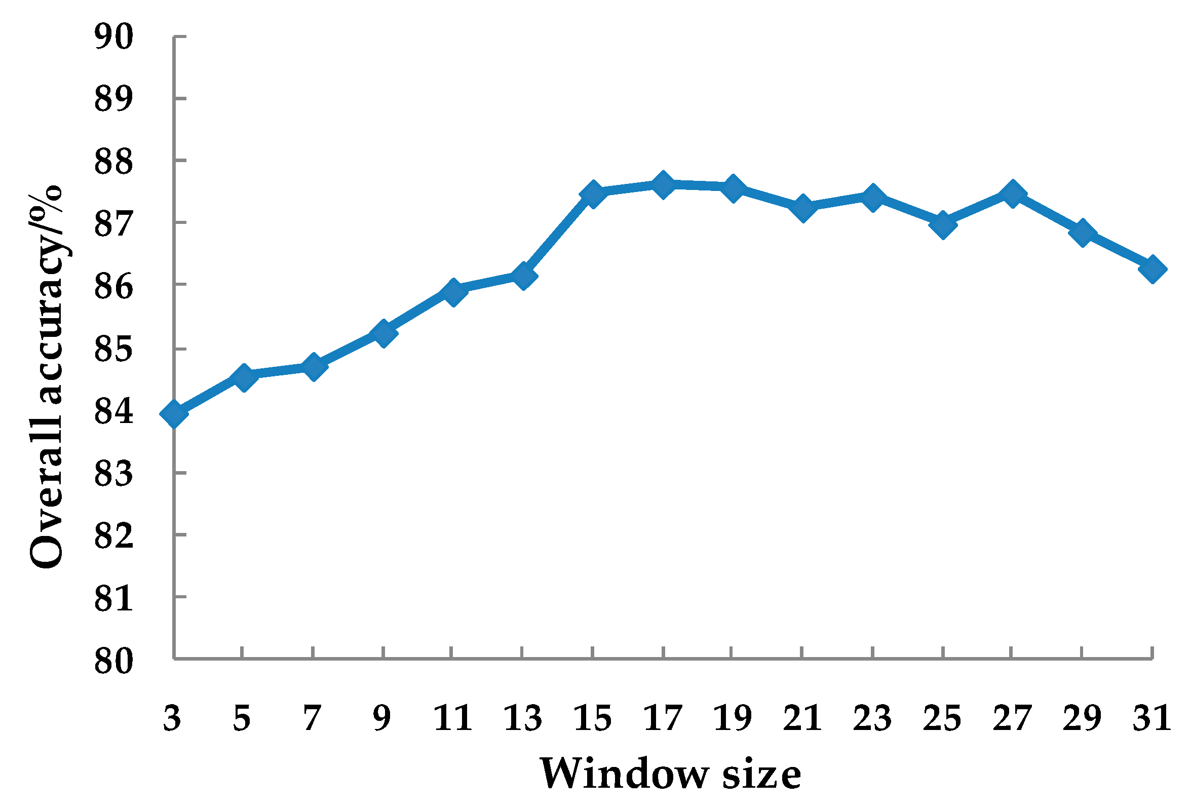
2.7.3. Textural Feature

Texture feature is an important factor in object-based classification [60,61]. Making full use of texture information of the image can effectively solve the phenomenon of the same objects with different spectrum. We used the grey level co-occurrence matrix (GLCM) to calculate eight texture features based on second-order matrix [62], including mean, variance (VAR), homogeneity (HOM), contrast (CON), dissimilarity (DIS), entropy (ENT), second moment (SM), and correlation (COR).
According to the previous studies [36,63], we selected three bands, i.e., band 482 nm, band 550 nm, and band 650 nm as RGB of hyperspectral images for texture analysis in this study. The texture window size was set from 3 × 3, 5 × 5, 7 × 7, …, to 31 × 31, and the step length was 1, the moving direction took the average of four directions of 0°, 45°, 90°, and 135°, to extract the above eight texture features. We selected different texture window size images to test the accuracy results by ICA transformation features selection and SVM classifier. As shown in Figure 6, the overall accuracy varied with the texture window size. When the window size was 17 × 17, the overall accuracy of classification is the highest. Therefore, we selected the 17 × 17 texture window size in this study and the extracted 24 texture features were used for the next feature combination and feature selection.

2.7.4. Canopy Height Model from LiDAR Data

The structure and height of tree species vary with their growth habits. Due to the phenomenon that different objects have the same spectrum, the tree species with similar spectral were difficult to distinguish [64,65]. In order to solve this problem, we used canopy height model obtained by LiDAR data as a feature variable, recorded the variable as the CHM, which reflected the height information of each tree species.
We calculated the CHM of each of the tree species samples, classified 1 m interval as one level, and obtained the tree species height distribution frequency chart (Figure 7). It can be seen that the height distribution curves of Illicium verum, masson pine, slash pine, Chinese fir, and mytilaria laosensis have obvious gaps and the height of eucalyptus species are not concentrated mainly due to different planting years. The other broad leaves include a variety of broadleaf species, therefore the height also distributes a wide range. According to statistics, the average tree height of each tree species is as follows: Illicium verum 5.01 m, masson pine 8.51 m, slash pine 14.82 m, Chinese fir 11.22 m, mytilaria laosensis 17.63 m, eucalyptus 13.47 m, and other broad leaves 16.25 m. It shows that the height information of different tree species is distinguishable.

2.7.5. Selection of Optimal Variable Combination

In this study, we extracted four sets of feature variables (Table 5), which constituted a larger dataset and increased the dimension of the data used for classification. These extracted feature variables could be highly correlated or redundant and increased the complexity of overall calculation. For some classifiers, it can lead to a dimensional disaster, called “Hughes phenomenon” [66]. For the classifier with Hughes phenomenon, the performance cannot reach the true expression [67], and therefore it is very important to avoid Hughes phenomenon. According to previous studies [68,69], feature selection in high-dimensional datasets and identification of the most important features can improve model interpretability and speed up the sample training process.
We used two methods to select feature variables. Random forest (RF) [68,70] is an algorithm based on decision trees. It modifies the candidate segmentation characteristics of decision trees, analyzes the results of each decision tree, and then completes the prediction and classification of samples. RF was used because it can rank the importance of all the feature variables, calculate the importance of each feature variable, and sort in descending order. The indicators include mean decrease accuracy (MDA) and mean decrease gini (MDG). Generally, the larger of the value means the variables are more important. On the basis of mean decrease accuracy, we selected the top-ranked feature variables as the optimal feature variables to participate in the classification.
Recursive feature elimination (RFE) is a feature selection method using feature ranking technology [71,72]. It performs the backward sequence reduction based on all of the input features, and eliminates the least relevant features each step, and finally, obtains the optimal feature subset [69]. On the basis of the SVM classifier, recursive feature elimination (SVM-RFE) was first applied to the field of molecular biology by Guyon et al. [73], and then applied to the field of remote sensing [74], but it was rarely applied in the classification of hyperspectral data. In this study, the SVM-RFE algorithm was used for feature selection. Through the comparison of all the features, the features with important functions were retained, and the features that had an inhibitory effect on the improvement of the classification accuracy were deleted. At the end, the optimal feature subset was formed.

2.8. Object-Based Classification

2.8.1. Classification Method

Object-based classification technology aggregates adjacent pixels with the same or similar attributes into one object, in which the image objects are used as the object-based classification unit [75]. On the basis of the segmentation objects, selected features are used for classification that can effectively distinguish categories. In this study, we used feature variables extracted from hyperspectral image and LiDAR data as the classification criteria, and selected k-nearest neighbor and support vector machine classifiers to classify tree species.
The k-nearest neighbor (KNN) is an instance-based learning method that is generally considered to be one of the simplest machine learning classifiers [36,76]. It has been widely used in high resolution and hyperspectral image classification [77]. The main idea of KNN classifier is to sort the difference between the calculated samples to be classified and the training samples, in ascending order, to select the top K least differential category. The category that has the most occurrences among the K categories is the most similar class. Finally, the samples are classified into classes with the most similar training samples. The optimal neighborhood value K of classification experiment is determined by performing multiple tests on training samples of different feature subsets.
Support vector machine (SVM) has been widely used in hyperspectral image classification as a supervised machine learning method based on statistical theory [78]. Its main idea is to maximize the distance between the two sides of the plane and the two types of samples closest to the plane by establishing an optimal decision hyperplane, providing a good generalization for classification. For a multidimensional sample set, the system randomly generates a hyperplane and moves continuously until the samples belonging to different categories are located on both sides of the hyperplane, which can solve the problem with a limited number of training samples and improve the generalization performance.

2.8.2. Determination of Classification Scheme

In order to evaluate the performance of different feature combinations and feature selection, six schemes were proposed for KNN and SVM object-based tree classification (Table 6).

2.8.3. Accuracy Assessment of Classification Results

The accuracy of KNN and SVM classifier classification results was evaluated using the selected 372 verification samples and the confusion matrix was used to evaluate the classification result of feature variables combination. The confusion matrix includes overall accuracy (OA), Kappa coefficients, producer accuracy (PA), and user accuracy (UA). Overall accuracy and Kappa coefficients are used for the overall classification performance. Producer accuracy and user accuracy are used to evaluate of individual classes [79].

3. Results

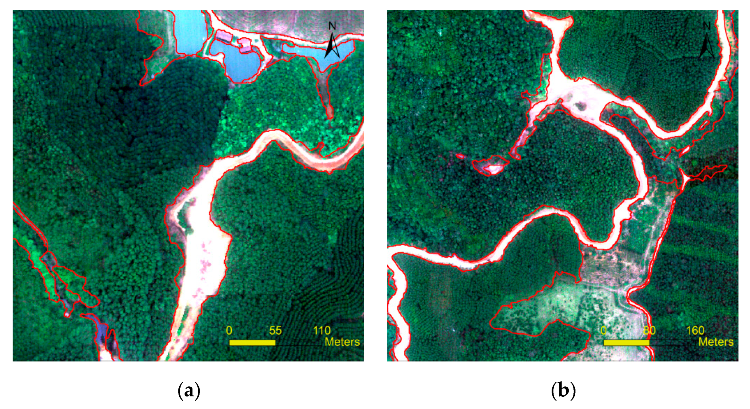
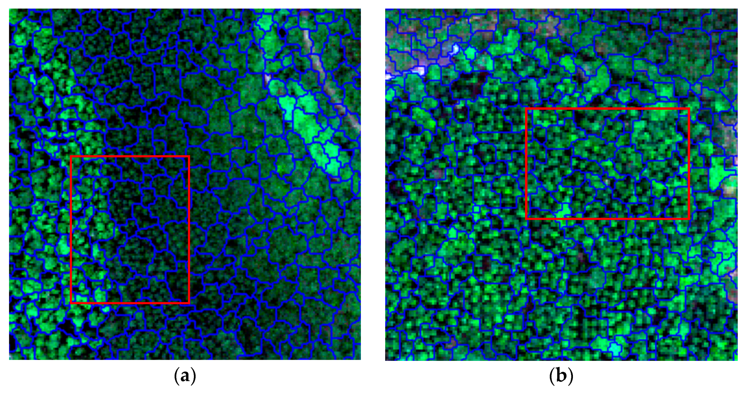
3.1. Image Segmentation Results

In the multiscale segmentation process, we need to set segmentation parameters, including weight of input layers, segmentation scale, shape index, and compactness. The scale of segmentation directly determines the size and fragmentation of the object. In general, the smaller the scale, the smaller the object, and the larger number of segments. First, we defined the range and step length of each parameter as follows: The range of scale was 1 to 5, step length was one, shape index ranged from 0.1 to 0.5, and compactness parameters ranged from 0.1 to 1, both of them had a step length of 0.1, and then we combined different parameters to segmented hyperspectral images.
We compared and analyzed all the segmentation results and found, when segmentation scale was four or five, that the Chinese fir, masson pine, and other broad-leaved tree species could not be separated well. When segmentation scale was one or two, segmented objects were too fragmented, which affected the image processing efficiency. According to a series of interactive segmentation experiments, we finally determined that when the segmentation scale was set to three, the shape index was set to 0.1, and the compactness was set to 0.4, the boundary of the segmented object best fits the boundary of actual tree species. As shown in Figure 8, each object includes a complete canopy or several canopies. Therefore, when we used these parameters to segment the hyperspectral image, the segmentation results were visually the best.

3.2. Extraction of Forest Land

Figure 9 shows the result of removing non-forest land and cutting land according to NDVI and CHM. The first step was to remove non-forest land. When the NDVI was <0.52 the water area, road, and buildings can be distinguished well. Therefore, we used 0.52 as the NDVI threshold to distinguish non-forest land. Secondly, in the forest land, there is also some forest land for seedling storage and cutting land, called other forest land. Generally, there are no trees or canopies in these land covers, therefore when 0.52 ≤ NDVI < 0.7 and CHM < 2, the other forest land can be better distinguished. Then, the rest are the forest land used to classify tree species. In order to facilitate observation, the forest land was merged. The left (Figure 9a) shows that water area and some road and buildings are better distinguished from the forest land. The right (Figure 9b) shows the distinguishing result between cutting land and the forest land. Therefore, stratified classification effectively avoids the mixing phenomenon of non-forest land and tree species.

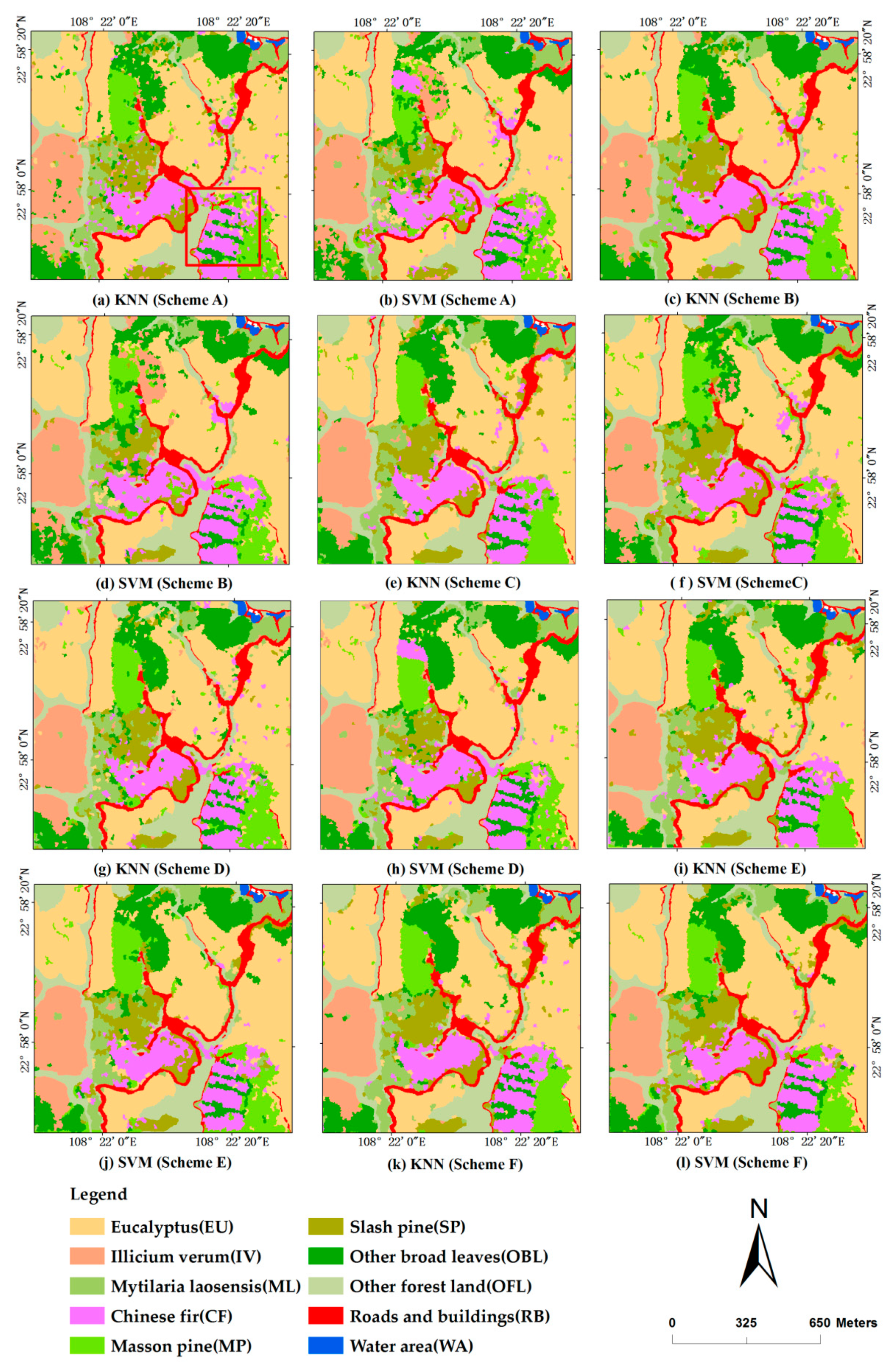
3.3. Comparison of Tree Species Classification Results

The classification results of different schemes using KNN and SVM classifiers are shown in Figure 10. Both classifiers spatially distinguish different tree species within the study area. According to the comparison and analysis of the classification results, the classification boundaries of eucalyptus and Chinese fir can be divided in space; whereas the Illicium verum and other broad-leaved species have obvious mixed phenomena in the first two schemes because the spectrum of the two tree species is similar. When texture features and CHM height information were added, the mixed phenomenon was greatly reduced. On both sides of the road, there are some mixed objects, the analysis is that the road and buildings have a certain influence on the spectral reflectance of trees and resulted in the mixed classification.
According to visual judgment, SVM classifier is better than KNN classifier. For example, some castanopsis hystrix intercroped with Chinese fir (the red polygon in the Figure 10) in the southeast corner of the study area can be better distinguished when using SVM classifier, while KNN classifier was trivially and misclassified some castanopsis hystrix into Chinese fir.
Table 7 summarizes the overall accuracy of the different classification schemes using KNN and SVM classifiers. The results show that SVM classifier is better than KNN classifier. On the basis of the SVM classifier, the scheme F classification accuracy is the best with the overall accuracy of 94.68%, and a Kappa coefficient of 0.937. The KNN classifier-based scheme D has the highest classification accuracy of 90.28% and a Kappa coefficient of 0.884. The classification accuracy was improved by 9.76% and 11.6% and the Kappa coefficients were improved by 0.117 and 0.139 as compared with scheme A based only on ICA transformation features.
The producer accuracy and user accuracy of different schemes based on the two classifiers are shown in Table 8 and Table 9.
For the classification scheme A based on ICA transformation features, the overall accuracy of the SVM classifier is 83.08% and the Kappa coefficient is 0.798; the overall accuracy of the KNN classifier is 80.51% and the Kappa coefficient is 0.767. Among them, the classification accuracy of eucalyptus is the highest, and the difference between its producer accuracy and user accuracy is very small, which shows that the results of these two classifiers for eucalyptus recognition is better and stable. Other broad-leaved species and slash pine have lower classification accuracy because the other broad-leaved species are mainly identified as Illicium verum and mytilaria laosensis. Because of the wide variety of other broad-leaved species, their spectral are very diverse; Illicium verum and mytilaria laosensis have similar spectral curves and many samples were misclassified into them.
After adding the spectral index features, the classification accuracy of the two classifiers was improved, and the overall accuracy was improved by 3.17% and 3.74%, respectively. The producer accuracy of slash pine increased the most, and the two classifiers were, respectively, improved from 62.09% and 71.25% to 81.17% and 90.08%. It indicates that the spectral index plays a certain role in tree species classification. The texture features were added to the classification scheme C, and the classification accuracy of each tree species was improved. The overall accuracy of the SVM classifier reaches 90.86%, and the accuracy of slash pine, masson pine, and Illicium verum species improved more than other species of broadleaf.
In the scheme D with added CHM features, the comparison of the classification accuracy of each tree species showed that the classification accuracy of other broad-leaved tree species is significantly improved. The producer accuracy of other broad-leaved tree species with the SVM classifier is 89.57%, i.e., improved by 15.24% and the KNN classifier is 81.68%, i.e., improved by 12.96%. The wide variety of other broad-leaved species have similar spectral curves with Illicium verum, and therefore most of them are misclassified into Illicium verum. The height of Illicium verum is lower at 5 meters, while the heights of other broad-leaved tree species are generally above 10 meters, and therefore after adding the height information, the separability of the two tree species was improved.
For scheme E and scheme F, the features selected by the random forest method and the recursive feature elimination method were used for classification. The classification accuracy of the KNN classifier used the selected features is close to the classification accuracy of all features, and the SVM classifier achieved higher classification accuracy as compared with using all the features. The comparison of the two feature selection methods showed that the recursive feature elimination based on SVM is slightly better than the random forest method and is more suitable for the classifier used in this study. In the selected two sets of feature subsets, there are 13 identical features selected by the two methods, among which there are nine spectral features. In the spectral indices, NDVI, PRI, GNDVI, SL2, and PSRI all appear in the two selected feature subsets.

4. Discussion

4.1. Comparison of Classification Results Based on Two Classifiers

In this study, object-based classification was used to classify tree species, and the classification effects of the two classifiers were compared and analyzed. As shown in Figure 10, SVM classifier can better distinguish castanopsis hystrix intercroped with Chinese fir, while KNN classifier has a trivial classification result with low classification accuracy, and some castanopsis hystrix are misclassified into Chinese fir. This is because KNN classifier is closely related to the distance of the training samples. For the strip-shaped castanopsis hystrix species, the objects to be classified are easily affected by the samples of Chinese fir, which leads to the misclassification. According to Table 7, the classification accuracy of SVM classifier is higher than KNN classifier. As a mature method in supervised classification, SVM requires low training samples and high operability. For multidimensional samples set, the system randomly generates a hyperplane and moves continuously, establishing an optimal decision hyperplane, and classifies the samples. Therefore, SVM classifier has good performance when the number of training samples was limited, which reduced misclassification. For example, slash pine and mytilaria laosensis have high producer accuracy and user accuracy. In scheme E and scheme F, the classification accuracy of the SVM classifier using the selected features is higher than using all the features. Similar conclusions were also obtained in previous studies [36,80], i.e., for excessive spectral features and other ancillary features, classifier performance and efficiency can be improved by eliminating redundant features.
With an increase of high spatial resolution images, more and more studies have adopted object-based methods. Previous studies have shown that object-based methods provide better classification accuracy than pixel-based methods when using high spatial resolution images [20]. In our study, we used object-based classification to avoid the phenomenon of “salt and pepper”, and effectively overcame the drawbacks by considering space, shape, and texture features of the image. However, there are some problems in the object-based method, which is that the segmentation scale parameters are difficult to determine adaptively, and the classification accuracy is affected by the segmentation accuracy. Therefore, rapid optimization and improvement of segmentation parameters are also important to improve classification accuracy.

4.2. The Role of Spectral Index Features

A comparison of the spectral reflectance curves of different tree species shows that the shape of the reflectance curve between conifers, conifers, and broad-leaved species is similar [35]. We also found that in the visible region, the reflectance difference between tree species is large, and in the near-infrared region, the reflectance difference between tree species is larger, and therefore this position is conducive to tree species identification. In view of that, we built the new spectral indices in the near-infrared region.
In this study, ICA transformation features and spectral indices extracted by hyperspectral imagery were used as spectral features. In scheme B, after adding spectral index features, the overall classification accuracies of two classifiers were improved by 3.17% and 3.74%, respectively. Scheme E and F used 13 identical features in the two subsets including nine spectral features, which indicates that the spectral features play an important role in the classification. In the spectral indices, NDVI, PRI, GNDVI, SL2, and PSRI appear in two subsets, which proves that the newly constructed index SL2 has an effect by improving the classification accuracy of tree species. The other selected indices, NDVI and GNDVI, are related to the chlorophyll content of plants. PRI is associated with changes in carotenoids in plants and PSRI is related to the ratio of carotenoids to chlorophyll. It indicates that the preferred spectral indices are closely related to the chlorophyll and carotenoids of the vegetation, while four indices are related to the vegetation reflectance in the near-infrared band. These factors can effectively distinguish different tree species. Therefore, spectral index, as a remote sensing parameter of vegetation, plays an important role in forest resource monitoring. In this study, we added spectral index features to classify tree species based on ICA transformation images. Previous studies have also shown that if the ground objects are subdivided such as tree species, it is difficult to identify tree species by spectral index alone [81]. Therefore, in practical applications, the use of spectral index combined with relevant auxiliary data is an effective method for extracting tree species information.

4.3. The Role of Texture Features

With the improvement of spatial resolution of remote sensing data, the use of spatial information is becoming more and more widely used while applying spectral information. Due to the different structure and growth state of the canopy, conifer and broadleaf species produce different texture features. In this study, texture information was added to the scheme C, and the classification accuracy of the two classifiers was significantly improved. The overall accuracy of the SVM classifier reaches 90.86%. It is explained that texture features play a role in classification. At present, there are many methods for texture analysis at home and abroad [82,83], among which the gray level co-ocurrence matrix (GLCM) is recognized as the most widely used and best applied method. In the process of extracting textures using GLCM, the results of texture extraction are closely related to different window sliding directions, window sliding distances, and window sizes. In this study, texture features of multiple texture window sizes were extracted, and we selected the 17 × 17 window size with the highest classification accuracy. The overall classification accuracy for slash pine, masson pine, and Illicium verum was higher than that of other species of broad leaves, which was related to the crown width of each tree species. The fact is that the canopy of the coniferous tree species is generally small, the height of the Illicium verum is low and the crown width is also small, and the crown width of other types of broad-leaved tree species is generally wide, showing that the texture window size we selected is more suitable for small crown tree species. Therefore, in subsequent studies, the tree species can be layered according to the characteristics of canopy, and then combined with different windows of the textures for classification.

4.4. The Role of Canopy Height Model

Airborne based hyperspectral imagery generally has high spatial resolution and spectral resolution and has obvious advantages in tree species identification [26]. However, using only hyperspectral imagery for vegetation classification results in different objects having the same spectrum and the same objects having different spectrum. Airborne LiDAR data can provide accurate three-dimensional structural information and has a good applicability for describing the vertical height of complex forest. The CHM extracted from LiDAR data is an important feature variable, and different tree species generally have a specific height range.
Previous studies have shown that combining canopy height characteristics can improve tree species classification [28,84]. In this study, scheme D added CHM height information, and the classification accuracy was improved as compared with the scheme without adding height information. The classification accuracy of other broad-leaved species is significantly increased with the improved producer accuracy of 15.24% and 12.96% by the SVM and KNN classifiers, respectively. This indicates that the addition of CHM features can effectively improve the classification accuracy of vegetation in complex forest areas, and it also shows that height information can play an important role when the spectral of tree species are similar. The addition of vertical structure information makes the training samples in relatively independent space and the interference factors less, and therefore the accuracy of the training samples is the key to improving the accuracy of image classification.
The height of the tree species can distinguish the tree species very well. One of the reasons is that the same tree species generally have the same forest age, and therefore the height information plays a greater role in improving the classification accuracy of the tree species. At the same time, we also found that the accuracy of eucalyptus decreased after adding height features due to the inconsistent height of the different planting years. Therefore, in applications, when distinguishing tree species in the stand in which each species has the same age group, the tree height can be utilized as a key feature variable, otherwise tree height information can produce extra disturbances which lead to low classification accuracy. In addition, the terrain of the study area selected in this study is relatively flat. The pixel values of the CHM can be used to indirectly reflect the vegetation height, which can effectively improve the accuracy of tree species classification. However, in hilly areas, the error of the point cloud data obtained from LiDAR data can increase, causing the generated DEM and DSM data to be inaccurate, and therefore the CHM may reflect incorrect tree heights. Therefore, in hilly areas, the impact of adding CHM data on classification accuracy of tree species needs further analysis. And different point cloud densities can create different CHM information. In subsequent studies, the impact of point cloud densities on tree species classification should be analyzed.
In general, spectral features, texture features, and CHM height information play a role in improving the classification accuracy of tree species. The addition of each feature increases the separability between categories. Among them, the height information has a significant effect on improving the classification accuracy of other broad-leaved species. When the spectral information of the tree species is similar, complete utilization of the height information and texture features can significantly improve the identification accuracy for the even-aged forest.

5. Conclusions

In this study, we used airborne hyperspectral images and LiDAR data for object-based tree classification. Independent components, spectral indices, and texture features were extracted from airborne hyperspectral data, new spectral indices were constructed by analyzing spectral curve of tree species, and CHM features were extracted from LiDAR data. On the basis of feature combination and feature selection, we compared and analyzed the contribution of different features and classifiers on object-based classification. The following conclusions can be drawn:
(1)
Compared with the KNN classifier, the SVM classifier has higher classification accuracy, with the highest classification accuracy of 94.68% and a Kappa coefficient of 0.937. It shows that the SVM classifier has better performance when the number of training samples is limited. By eliminating redundant features, the classification accuracy and performance of the SVM classifier can be further improved, and the recursive feature elimination based on the SVM feature selection method is better than random forest.
(2)
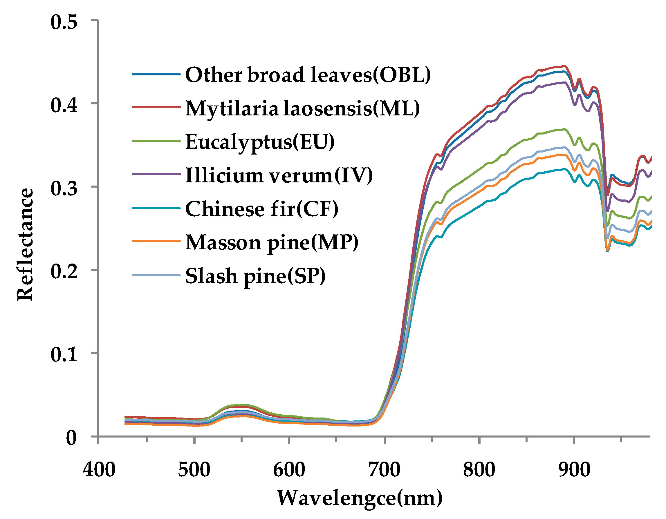
In the spectral indices, NDVI, PRI, GNDVI, SL2, and PSRI are in the selected feature subsets, indicating that the newly constructed SL2 spectral index plays a role in improving classification accuracy. At the same time, the preferred spectral indices are closely related to vegetation chlorophyll and carotenoids, and four indices are related to near-infrared band. These factors can effectively distinguish different tree species.
(3)
With the addition of texture features, the classification accuracy of both classifiers is significantly improved. The overall classification accuracy of slash pine, masson pine, and Illicium verum was higher than other species of broad leaves. Therefore, the selected texture window size is more suitable for small crown tree species, which implies that using a single texture window size has certain limitations. Considering the type of forest, using multiscale texture window size should be a new research topic in improving tree species classification.
(4)
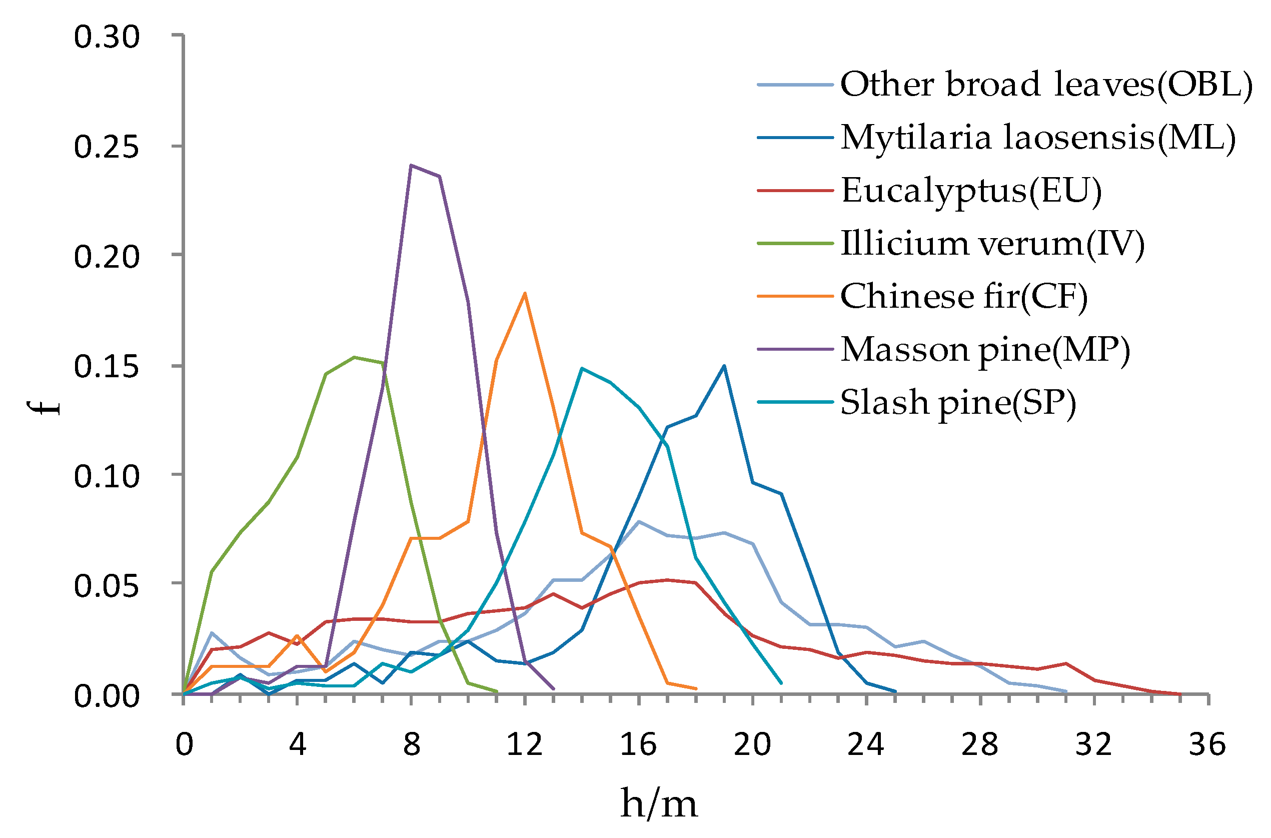
CHM height information has a significant effect on improving the classification accuracy of tree species especially other broad-leaved species. It can effectively distinguish tree species with similar spectral features, but different tree heights. The accuracy of the CHM is affected by the terrain. In hilly areas, the CHM may reflect incorrect tree heights. In addition, the CHM has a certain relationship with the LiDAR point cloud density, and therefore the influence of point cloud density and terrain factors on CHM and tree species classification need further analysis.
(5)
Object-based classification can avoid the phenomenon of “salt and pepper” and classification accuracy is affected by the segmentation accuracy. However, segmentation scale parameters are difficult to determine adaptively, so rapid optimization and improvement of segmentation parameters are quite important to improve classification accuracy.

Author Contributions

Conceptualization, X.Z.; data curation, Y.W.; investigation, Y.W.; methodology, X.Z. and Y.W.; resources, X.Z. and Y.W.; formal analysis, Y.W.; supervision, X.Z.; validation, Y.W.; writing–original draft, Y.W.; writing–review and editing, X.Z.; project administration, X.Z. All authors have read and agreed to the published version of the manuscript.

Funding

This research is financially supported by the National Key R&D Program of China project “Research of Key Technologies for Monitoring Forest Plantation Resources” (2017YFD0600900).

Acknowledgments

The authors would like to thank Lin Zhao, Jian Zeng, Zhenfeng Sun, Yufeng Zheng, Zhengqi Guo, Wenting Guo, Kaili Cao, Niwen Li, Xuemei Zhou, Langning Huo, Xiaomin Tian, Linghan Gao, and Bin Zhang for their help in the fieldwork.

Conflicts of Interest

The authors declare no conflict of interest.

References

  1. Li, D.; Fan, S.; He, A.; Yin, F. Forest resources and environment in China. J. For. Res. 2004, 9, 307–312. [Google Scholar] [CrossRef]
  2. Cheng, S.; Xu, Z.; Su, Y.; Zhen, L. Spatial and temporal flows of China’s forest resources: Development of a framework for evaluating resource efficiency. Ecol. Econ. 2010, 69, 1405–1415. [Google Scholar] [CrossRef]
  3. Brockerhoff, E.G.; Jactel, H.; Parrotta, J.A.; Quine, C.P.; Sayer, J. Plantation forests and biodiversity: Oxymoron or opportunity? Biodivers. Conserv. 2008, 17, 925–951. [Google Scholar] [CrossRef]
  4. Yang, J.; Wang, F. Developing a quantitative index system for assessing sustainable forestry management in Heilongjiang Province, China: A case study. J. For. Res. 2016, 27, 611–619. [Google Scholar] [CrossRef]
  5. Liu, S.; Xia, C.; Feng, W.; Zhang, K.; Ma, L.; Liu, J. Estimation of vegetation carbon storage and density of forests at tree layer in Tibet, China. Chin. J. Appl. Ecol. 2017, 28, 3127–3134. [Google Scholar] [CrossRef]
  6. Adams, A.B.; Pontius, J.; Galford, G.L.; Merrill, S.C.; Gudex-Cross, D. Modeling carbon storage across a heterogeneous mixed temperate forest: The influence of forest type specificity on regional-scale carbon storage estimates. Landsc. Ecol. 2018, 33, 641–658. [Google Scholar] [CrossRef]
  7. Fassnacht, F.E.; Latifi, H.; Sterenczak, K.; Modzelewska, A.; Lefsky, M.; Waser, L.T.; Straub, C.; Ghosh, A. Review of studies on tree species classification from remotely sensed data. Remote Sens. Environ. 2016, 186, 64–87. [Google Scholar] [CrossRef]
  8. Ni, X.; Zhou, Y.; Cao, C.; Wang, X.; Shi, Y.; Park, T.; Choi, S.; Myneni, R.B. Mapping Forest Canopy Height over Continental China Using Multi-Source Remote Sensing Data. Remote Sens. 2015, 7, 8436–8452. [Google Scholar] [CrossRef] [Green Version]
  9. Kempeneers, P.; Sedano, F.; Seebach, L.; Strobl, P.; San-Miguel-Ayanz, J. Data Fusion of Different Spatial Resolution Remote Sensing Images Applied to Forest-Type Mapping. IEEE Trans. Geosci. Remote Sens. 2011, 49, 4977–4986. [Google Scholar] [CrossRef]
  10. Zhu, X.; Liu, D. Accurate mapping of forest types using dense seasonal Landsat time-series. ISPRS J. Photogramm. Remote Sens. 2014, 96, 1–11. [Google Scholar] [CrossRef]
  11. Gong, P.; Pu, R.; Yu, B. Conifer species recognition with seasonal hyperspectral data. J. Remote Sens. 1998, 2, 211–217. [Google Scholar] [CrossRef]
  12. Shen, X.; Cao, L. Tree-Species Classification in Subtropical Forests Using Airborne Hyperspectral and LiDAR Data. Remote Sens. 2017, 9, 1180. [Google Scholar] [CrossRef] [Green Version]
  13. Zhang, Z.; Kazakova, A.; Moskal, L.M.; Styers, D.M. Object-Based Tree Species Classification in Urban Ecosystems Using LiDAR and Hyperspectral Data. Forests 2016, 7, 122. [Google Scholar] [CrossRef] [Green Version]
  14. Zhang, J.; Rivard, B.; Sanchez-Azofeifa, A.; Castro-Esau, K. Intra and inter-class spectral variability of tropical tree species at La Selva, Costa Rica: Implications for species identification using HYDICE imagery. Remote Sens. Environ. 2006, 105, 129–141. [Google Scholar] [CrossRef]
  15. Dian, Y.; Li, Z.; Pang, Y. Spectral and Texture Features Combined for Forest Tree species Classification with Airborne Hyperspectral Imagery. J. Indian Soc. Remote Sens. 2015, 43, 101–107. [Google Scholar] [CrossRef]
  16. Fagan, M.E.; DeFries, R.S.; Sesnie, S.E.; Arroyo-Mora, J.P.; Soto, C.; Singh, A.; Townsend, P.A.; Chazdon, R.L. Mapping Species Composition of Forests and Tree Plantations in Northeastern Costa Rica with an Integration of Hyperspectral and Multitemporal Landsat Imagery. Remote Sens. 2015, 7, 5660–5696. [Google Scholar] [CrossRef] [Green Version]
  17. Johansen, K.; Phinn, S. Mapping structural parameters and species composition of riparian vegetation using IKONOS and landsat ETM plus data in Australian tropical savannahs. Photogramm. Eng. Remote Sens. 2006, 72, 71–80. [Google Scholar] [CrossRef]
  18. Du, P.; Xia, J.; Zhang, W.; Tan, K.; Liu, Y.; Liu, S. Multiple Classifier System for Remote Sensing Image Classification: A Review. Sensors 2012, 12, 4764–4792. [Google Scholar] [CrossRef]
  19. Wu, Q.; Zhong, R.; Zhao, W.; Fu, H.; Song, K. A comparison of pixel-based decision tree and object-based Support Vector Machine methods for land-cover classification based on aerial images and airborne lidar data. Int. J. Remote Sens. 2017, 38, 7176–7195. [Google Scholar] [CrossRef]
  20. Kaszta, Z.; Van de Kerchove, R.; Ramoelo, A.; Cho, M.A.; Madonsela, S.; Mathieu, R.; Wolff, E. Seasonal Separation of African Savanna Components Using Worldview-2 Imagery: A Comparison of Pixel- and Object-Based Approaches and Selected Classification Algorithms. Remote Sens. 2016, 8, 763. [Google Scholar] [CrossRef] [Green Version]
  21. Pu, R.; Landry, S. A comparative analysis of high spatial resolution IKONOS and WorldView-2 imagery for mapping urban tree species. Remote Sens. Environ. 2012, 124, 516–533. [Google Scholar] [CrossRef]
  22. Kavzoglu, T.; Erdemir, M.Y.; Tonbul, H. Classification of semiurban landscapes from very high-resolution satellite images using a regionalized multiscale segmentation approach. J. Appl. Remote Sens. 2017, 11. [Google Scholar] [CrossRef]
  23. Byun, Y.G.; Han, Y.K.; Chae, T.B. A multispectral image segmentation approach for object-based image classification of high resolution satellite imagery. Ksce. J. Civ. Eng. 2013, 17, 486–497. [Google Scholar] [CrossRef]
  24. Immitzer, M.; Atzberger, C.; Koukal, T. Tree Species Classification with Random Forest Using Very High Spatial Resolution 8-Band WorldView-2 Satellite Data. Remote Sens. 2012, 4, 2661–2693. [Google Scholar] [CrossRef] [Green Version]
  25. Wang, Z.; Shi, J.; Yue, G.; Zhao, L.; Nan, Z.; Wu, X.; Qiao, Y.; Wu, T.; Zou, D. Object-Oriented Vegetation Classification Based on Fusion Decision Tree Method in Yushu Area. Acta Prataculturae Sin. 2013, 22, 62–71. [Google Scholar]
  26. Fauvel, M.; Tarabalka, Y.; Benediktsson, J.A.; Chanussot, J.; Tilton, J.C. Advances in Spectral-Spatial Classification of Hyperspectral Images. Proc. IEEE 2013, 101, 652–675. [Google Scholar] [CrossRef] [Green Version]
  27. Ghosh, A.; Fassnacht, F.E.; Joshi, P.K.; Koch, B. A framework for mapping tree species combining hyperspectral and LiDAR data: Role of selected classifiers and sensor across three spatial scales. Int. J. Appl. Earth Obs. Geoinf. 2014, 26, 49–63. [Google Scholar] [CrossRef]
  28. Liu, L.; Coops, N.C.; Aven, N.W.; Pang, Y. Mapping urban tree species using integrated airborne hyperspectral and LiDAR remote sensing data. Remote Sens. Environ. 2017, 200, 170–182. [Google Scholar] [CrossRef]
  29. Hollaus, M.; Wagner, W.; Eberhoefer, C.; Karel, W. Accuracy of large-scale canopy heights derived from LiDAR data under operational constraints in a complex alpine environment. ISPRS J. Photogramm. Remote Sens. 2006, 60, 323–338. [Google Scholar] [CrossRef]
  30. Heinzel, J.; Koch, B. Exploring full-waveform LiDAR parameters for tree species classification. Int. J. Appl. Earth Obs. Geoinf. 2011, 13, 152–160. [Google Scholar] [CrossRef]
  31. Alonzo, M.; Bookhagen, B.; Roberts, D.A. Urban tree species mapping using hyperspectral and lidar data fusion. Remote Sens. Environ. 2014, 148, 70–83. [Google Scholar] [CrossRef]
  32. Colgan, M.S.; Baldeck, C.A.; Feret, J.B.; Asner, G.P. Mapping Savanna Tree Species at Ecosystem Scales Using Support Vector Machine Classification and BRDF Correction on Airborne Hyperspectral and LiDAR Data. Remote Sens. 2012, 4, 3462–3480. [Google Scholar] [CrossRef] [Green Version]
  33. Shi, Y.; Skidmore, A.K.; Wang, T.; Holzwarth, S.; Heiden, U.; Pinnel, N.; Zhu, X.; Heurich, M. Tree species classification using plant functional traits from LiDAR and hyperspectral data. Int. J. Appl. Earth Obs. Geoinf. 2018, 73, 207–219. [Google Scholar] [CrossRef]
  34. Voss, M.; Sugumaran, R. Seasonal effect on tree species classification in an urban environment using hyperspectral data, LiDAR, and an object-oriented approach. Sensors 2008, 8, 3020–3036. [Google Scholar] [CrossRef] [PubMed] [Green Version]
  35. Liu, L.; Pang, Y.; Fan, W.; Li, Z.; Zhang, D.; Li, M. Fused airborne LiDAR and hyperspectral data for tree species identification in a natural temperate forest. J. Remote Sens. 2013, 17, 679–695. [Google Scholar]
  36. Cao, J.; Leng, W.; Liu, K.; Liu, L.; He, Z.; Zhu, Y. Object-Based Mangrove Species Classification Using Unmanned Aerial Vehicle Hyperspectral Images and Digital Surface Models. Remote Sens. 2018, 10, 89. [Google Scholar] [CrossRef] [Green Version]
  37. Pan, Z.; Luo, L. Peak of State-owned Forest Farms in Guangxi the Characteristics of Different Tree Species Forests Soil Research. J. Green Sci. Technol. 2017, 3, 116–118. [Google Scholar] [CrossRef]
  38. Mo, W.; Chen, J.; Tang, X. Thoughts and Suggestions on the Development of Under-forest Economy in Gaofeng Forest Farm. For. Econ. 2018, 40, 106–110. [Google Scholar] [CrossRef]
  39. Introduction of Gaofeng Forest Farm. Available online: http://www.gaofenglinye.com.cn/lcjj/index_13.aspx (accessed on 30 January 2019).
  40. Pang, Y.; Li, Z.; Ju, H.; Lu, H.; Jia, W.; Si, L.; Guo, Y.; Liu, Q.; Li, S.; Liu, L.; et al. LiCHy: The CAF’s LiDAR, CCD and Hyperspectral Integrated Airborne Observation System. Remote Sens. 2016, 8, 398. [Google Scholar] [CrossRef] [Green Version]
  41. AISA Eagle II. Available online: http://www.specim.fi/hyperspectral-remote-sensing/ (accessed on 30 January 2019).
  42. RIEGL LMS-Q680i. Available online: http://www.riegl.com/nc/products/airborne-scanning/ (accessed on 30 January 2019).
  43. DigiCAM-Digital Aerial Camera. Available online: https://www.igi-systems.com/digicam.html (accessed on 30 January 2019).
  44. Hao, J.; Yang, W.; Li, Y.; Hao, J. Atmospheric Correction of Multi-spectral Imagery ASTER. Remote Sens. Inf. 2008, 1, 78–81. [Google Scholar] [CrossRef]
  45. Axelsson, P. Processing of laser scanner data—Algorithms and applications. ISPRS J. Photogramm. Remote Sens. 1999, 54, 138–147. [Google Scholar] [CrossRef]
  46. Liu, Y.; Pang, Y.; Liao, S.; Jia, W.; Chen, B.; Liu, L. Merged Airborne LiDAR and Hyperspectral Data for Tree Species Classification in Puer’s Mountainous Area. For. Res. 2016, 29, 407–412. [Google Scholar] [CrossRef]
  47. Li, N.; Lu, D.; Wu, M.; Zhang, Y.; Lu, L. Coastal wetland classification with multiseasonal high-spatial resolution satellite imagery. Int. J. Remote Sens. 2018, 39, 8963–8983. [Google Scholar] [CrossRef]
  48. Labib, S.M.; Harris, A. The potentials of Sentinel-2 and LandSat-8 data in green infrastructure extraction, using object based image analysis (OBIA) method. Eur. J. Remote Sens. 2018, 51, 231–240. [Google Scholar] [CrossRef]
  49. Jiang, Z.; Huete, A.R.; Li, J.; Chen, Y. An analysis of angle-based with ratio-based vegetation indices. IEEE. Trans. Geosci. Remote Sens. 2006, 44, 2506–2513. [Google Scholar] [CrossRef]
  50. Koller, M.; Upadhyaya, S.K. Relationship between modified normalized difference vegetation index and leaf area index for processing tomatoes. Appl. Eng. Agric. 2005, 21, 927–933. [Google Scholar] [CrossRef]
  51. Omam, M.A.; Torkamani-Azar, F. Band selection of hyperspectral-image based weighted indipendent component analysis. Opt. Rev. 2010, 17, 367–370. [Google Scholar] [CrossRef]
  52. Lichtenthaler, H.; Lang, M.; Sowinska, M.; Heisel, F.; Miehe, J. Detection of vegetation stress via a new high resolution fluorescence imaging system. J. Plant. Physiol. 1996, 148, 599–612. [Google Scholar] [CrossRef]
  53. Bannari, A.; Morin, D.; Bonn, F.; Huete, A.R. A review of vegetation indices. Remote Sens. Rev. 1995, 13, 95–120. [Google Scholar] [CrossRef]
  54. Merzlyak, M.N.; Gitelson, A.A.; Chivkunova, O.B.; Rakitin, V.Y. Non-destructive optical detection of pigment changes during leaf senescence and fruit ripening. Physiol. Plant. 1999, 106, 135–141. [Google Scholar] [CrossRef] [Green Version]
  55. Sims, D.A.; Gamon, J.A. Relationships between leaf pigment content and spectral reflectance across a wide range of species, leaf structures and developmental stages. Remote Sens. Environ. 2002, 81, 337–354. [Google Scholar] [CrossRef]
  56. Hernandez-Clemente, R.; Navarro-Cerrillo, R.M.; Suarez, L.; Morales, F.; Zarco-Tejada, P.J. Assessing structural effects on PRI for stress detection in conifer forests. Remote Sens. Environ. 2011, 115, 2360–2375. [Google Scholar] [CrossRef]
  57. Haboudane, D.; Miller, J.R.; Tremblay, N.; Zarco-Tejada, P.J.; Dextraze, L. Integrated narrow-band vegetation indices for prediction of crop chlorophyll content for application to precision agriculture. Remote Sens. Environ. 2002, 81, 416–426. [Google Scholar] [CrossRef]
  58. Xue, J.; Su, B. Significant Remote Sensing Vegetation Indices: A Review of Developments and Applications. J. Sens. 2017, 2017. [Google Scholar] [CrossRef] [Green Version]
  59. Gitelson, A.A.; Merzlyak, M.N.; Chivkunova, O.B. Optical properties and nondestructive estimation of anthocyanin content in plant leaves. Photochem. Photobiol. 2001, 74, 38–45. [Google Scholar] [CrossRef]
  60. Huang, X.; Lu, Q.; Zhang, L. A multi-index learning approach for classification of high-resolution remotely sensed images over urban areas. ISPRS J. Photogramm. Remote Sens. 2014, 90, 36–48. [Google Scholar] [CrossRef]
  61. Lu, D.; Li, G.; Moran, E.; Dutra, L.; Batistella, M. The roles of textural images in improving land-cover classification in the Brazilian Amazon. Int. J. Remote Sens. 2014, 35, 8188–8207. [Google Scholar] [CrossRef] [Green Version]
  62. Wang, H.; Zhao, Y.; Pu, R.; Zhang, Z. Mapping Robinia Pseudoacacia Forest Health Conditions by Using Combined Spectral, Spatial, and Textural Information Extracted from IKONOS Imagery and Random Forest Classifier. Remote Sens. 2015, 7, 9020–9044. [Google Scholar] [CrossRef] [Green Version]
  63. Pu, R.; Gong, P. Hyperspectral remote sensing of vegetation bioparameters. Adv. Environ. Remote Sens. 2011, 7, 101–142. [Google Scholar]
  64. Dalponte, M.; Bruzzone, L.; Gianelle, D. Fusion of hyperspectral and LIDAR remote sensing data for classification of complex forest areas. IEEE Trans. Geosci. Remote Sens. 2008, 46, 1416–1427. [Google Scholar] [CrossRef] [Green Version]
  65. Goetze, C.; Gerstmann, H.; Glaesser, C.; Jung, A. An approach for the classification of pioneer vegetation based on species-specific phenological patterns using laboratory spectrometric measurements. Phys. Geogr. 2017, 38, 524–540. [Google Scholar] [CrossRef]
  66. Batista, M.H.; Haertel, V. On the classification of remote sensing high spatial resolution image data. Int. J. Remote Sens. 2010, 31, 5533–5548. [Google Scholar] [CrossRef]
  67. Liu, H.; An, H.; Wang, B.; Zhang, Q. WorldView-2 Tree Classification Based on Recursive Texture Feature Elimination. J. Beijing For. Univ. 2015, 37, 53–59. [Google Scholar]
  68. Liao, W.; Pizurica, A.; Scheunders, P.; Philips, W.; Pi, Y. Semisupervised local discriminant analysis for feature extraction in hyperspectral images. IEEE Trans. Geosci. Remote Sens. 2013, 51, 184–198. [Google Scholar] [CrossRef]
  69. Hu, S.; Liu, H.; Zhao, W.; Shi, T.; Hu, Z.; Li, Q.; Wu, G. Comparison of Machine Learning Techniques in Inferring Phytoplankton Size Classes. Remote Sens. 2018, 10, 191. [Google Scholar] [CrossRef] [Green Version]
  70. Dye, M.; Mutanga, O.; Ismail, R. Examining the utility of random forest and AISA Eagle hyperspectral image data to predict Pinus patula age in KwaZulu-Natal, South Africa. Geocarto Int. 2011, 26, 275–289. [Google Scholar] [CrossRef]
  71. Huang, X.; Zhang, L.; Wang, B.; Li, F.; Zhang, Z. Feature clustering based support vector machine recursive feature elimination for gene selection. Appl. Intell. 2018, 48, 594–607. [Google Scholar] [CrossRef]
  72. Schultz, B.; Immitzer, M.; Formaggio, A.R.; Sanches, I.D.A.; Barreto Luiz, A.J.; Atzberger, C. Self-Guided Segmentation and Classification of Multi-Temporal Landsat 8 Images for Crop Type Mapping in Southeastern Brazil. Remote Sens. 2015, 7, 14482–14508. [Google Scholar] [CrossRef] [Green Version]
  73. Guyon, I.; Weston, J.; Barnhill, S.; Vapnik, V. Gene selection for cancer classification using support vector machines. Mach. Learn. 2002, 46, 389–422. [Google Scholar] [CrossRef]
  74. Immitzer, M.; Böck, S.; Einzmann, K.; Vuolo, F.; Pinnel, N.; Wallner, A.; Atzberger, C. Fractional cover mapping of spruce and pine at 1 ha resolution combining very high and medium spatial resolution satellite imagery. Remote Sens. Environ. 2018, 204, 690–703. [Google Scholar] [CrossRef] [Green Version]
  75. Cai, S.; Liu, D. A comparison of object-based and contextual pixel-based classifications using high and medium spatial resolution images. Remote Sens. Lett. 2013, 4, 998–1007. [Google Scholar] [CrossRef]
  76. Cover, T.; Hart, P. Nearest neighbor pattern classification. IEEE Trans. Inf. Theory 1967, 13, 21–27. [Google Scholar] [CrossRef]
  77. Yang, J.M.; Yu, P.T.; Kuo, B.C. A Nonparametric Feature Extraction and Its Application to Nearest Neighbor Classification for Hyperspectral Image Data. IEEE Trans. Geosci. Remote Sens. 2010, 48, 1279–1293. [Google Scholar] [CrossRef]
  78. Xun, L.; Wang, L. An object-based SVM method incorporating optimal segmentation scale estimation using Bhattacharyya Distance for mapping salt cedar (Tamarisk spp.) with QuickBird imagery. GIsci. Remote Sens. 2015, 52, 257–273. [Google Scholar] [CrossRef]
  79. Congalton, R.G.; Green, K. Assessing the Accuracy of Remotely Sensed Data: Principles and Practices, 2nd ed.; CRC Press: Boca Raton, FL, USA, 2008. [Google Scholar]
  80. Ma, L.; Cheng, L.; Li, M.; Liu, Y.; Ma, X. Training set size, scale, and features in Geographic Object-Based Image Analysis of very high resolution unmanned aerial vehicle imagery. ISPRS J. Photogramm. Remote Sens. 2015, 102, 14–27. [Google Scholar] [CrossRef]
  81. Maschler, J.; Atzberger, C.; Immitzer, M. Individual Tree Crown Segmentation and Classification of 13 Tree Species Using Airborne Hyperspectral Data. Remote Sens. 2018, 10, 1218. [Google Scholar] [CrossRef] [Green Version]
  82. Feng, Q.; Liu, J.; Gong, J. UAV Remote Sensing for Urban Vegetation Mapping Using Random Forest and Texture Analysis. Remote Sens. 2015, 7, 1074–1094. [Google Scholar] [CrossRef] [Green Version]
  83. Su, W.; Zhang, C.; Yang, J.; Wu, H.; Deng, L.; Ou, W.; Yue, A.; Chen, M. Analysis of wavelet packet and statistical textures for object-oriented classification of forest-agriculture ecotones using SPOT 5 imagery. Int. J. Remote Sens. 2012, 33, 3557–3579. [Google Scholar] [CrossRef]
  84. Dian, Y.; Pang, Y.; Dong, Y.; Li, Z. Urban Tree Species Mapping Using Airborne LiDAR and Hyperspectral Data. J. Indian Soc. Remote Sens. 2016, 44, 595–603. [Google Scholar] [CrossRef]
Figure 1. Location of the Jiepai Forest Farm, the CCD orthoimage of the Jiepai Forest Farm (blue polygon) and the location of the study area (yellow polygon), the hyperspectral image (upper right) and the LiDAR CHM image (lower right) of the study area.
Forests 11 00032 g001
Figure 2. Mean spectral reflectance curves of the seven tree species in the study site.
Forests 11 00032 g002
Figure 3. Workflow for object-based tree species classification based on airborne hyperspectral image and LiDAR data.
Forests 11 00032 g003
Figure 4. Schematic diagram of spectral curves slope and area between different tree species.
Forests 11 00032 g004
Figure 5. The first derivative curves between different tree species.
Forests 11 00032 g005
Figure 6. Influence of texture window size on classification overall accuracy.
Forests 11 00032 g006
Figure 7. Distribution frequency chart of height for tree species.
Forests 11 00032 g007
Figure 8. The image segmentation results. (a) The segmentation effect of the boundary of the two tree species and (b) the segmentation effect of the pure forest land.
Forests 11 00032 g008
Figure 9. The result of stratified classification. (a) Water area and road and buildings distinguished from the forest land and (b) the distinction result between cutting land and the forest land.
Forests 11 00032 g009
Figure 10. Classification results of different schemes using the KNN and SVM classifiers. (a) Scheme A by KNN classifier, (b) scheme A by SVM classifier, (c) scheme B by KNN classifier, (d) scheme B by SVM classifier, (e) scheme C by KNN classifier, (f) scheme C by SVM classifier, (g) scheme D by KNN classifier, (h) scheme D by SVM classifier, (i) scheme E by KNN classifier, (j) scheme E by SVM classifier, (k) scheme F by KNN classifier, and (l) scheme F by SVM classifier.
Forests 11 00032 g010
Table 1. Classification system of the study area.
TypeCommon NameAcronymScientific Name
Non-forest landWater areaWA-
Roads and buildingsRB-
Forest landOther forest landOFL-
Chinese firCFCunninghamia lanceolata (Lamb.) Hook.
EucalyptusEUEucalyptus robusta Smith
Illicium verumIVIllicium verum Hook.f.
Mytilaria laosensisMLMytilaria laosensis Lec.
Slash pinePEPinus elliottii Engelm.
Masson pineMPPinus massoniana Lamb.
Other broad leavesOBL-
Table 2. The parameters of the three earth observation sensors in the LiCHy system. Adapted from [40], with permission from MDPI journals, 2016.
Hyperspectral: AISA Eagle II
Spectral range400~1000 nmSpatial resolution1 m
Spectral resolution3.3 nmSpectral bands125
FOV37.7°Spatial pixels1024
IFOV0.646 mradSpectral sampling interval4.6 nm
Focal length18.5 mmBit depth12 bits
LiDAR: Riegl LMS-Q680i
Wavelength1550 nmLaser beam divergence0.5 mrad
Laser pulse length3 nsCross-track FOV±30°
Maximum laser pulse repetition rate400 KHzVertical resolution0.15 m
Waveform sampling interval1 nsPoint density3.6 pts/m2
CCD: DigiCAM-60
Frame size8956 × 6708Pixel size6 µm
Imaging sensor size40.30 mm × 53.78 mmBit depth16 bits
FOV56.2°Focal length50 mm
Spatial resolution0.2 m
Table 3. Number of samples for training and validation for each tree species.
Tree SpeciesTraining SamplesVerification Samples
Image ObjectsNumber of PixelsImage ObjectsNumber of Pixels
Illicium verum (IV)65326749646
Masson pine (MP)62311643555
Slash pine (SP)45226231393
Chinese fir (CF)64321745580
Mytilaria laosensis (ML)58291549624
Eucalyptus (EU)1537691971247
Other broad leaves (OBL)75377058748
Total52226,2383724793
Table 4. The spectral indices equation calculated by hyperspectral images.
Spectral IndicesEquation
Normalized difference vegetation index NDVI = ( ρ 800 ρ 678 ) / ( ρ 800 + ρ 678 )
Plant senescence reflectance index PSRI = ( ρ 680 ρ 501 ) / ρ 750
Modified red edge simple ratio index MRESRI = ( ρ 750 ρ 445 ) / ( ρ 705 + ρ 445 )
Modified red edge normalized difference vegetation index MRENDVI = ( ρ 750 ρ 705 ) ( ρ 750 + ρ 705 2 ρ 445 )
Normalized green difference vegetation index GNDVI = ( ρ 800 ρ 546 ) / ( ρ 800 + ρ 546 )
Photochemical reflectance index PRI = ( ρ 531 ρ 570 ) / ( ρ 531 + ρ 570 )
Structure insensitive pigment index SIPI = ( ρ 800 ρ 445 ) / ( ρ 800 + ρ 680 )
Anthocyanin reflectance index ARI 1 = 1 ρ 550 1 ρ 700
Vogelmann red edge index VOG 1 = ρ 740 / ρ 720
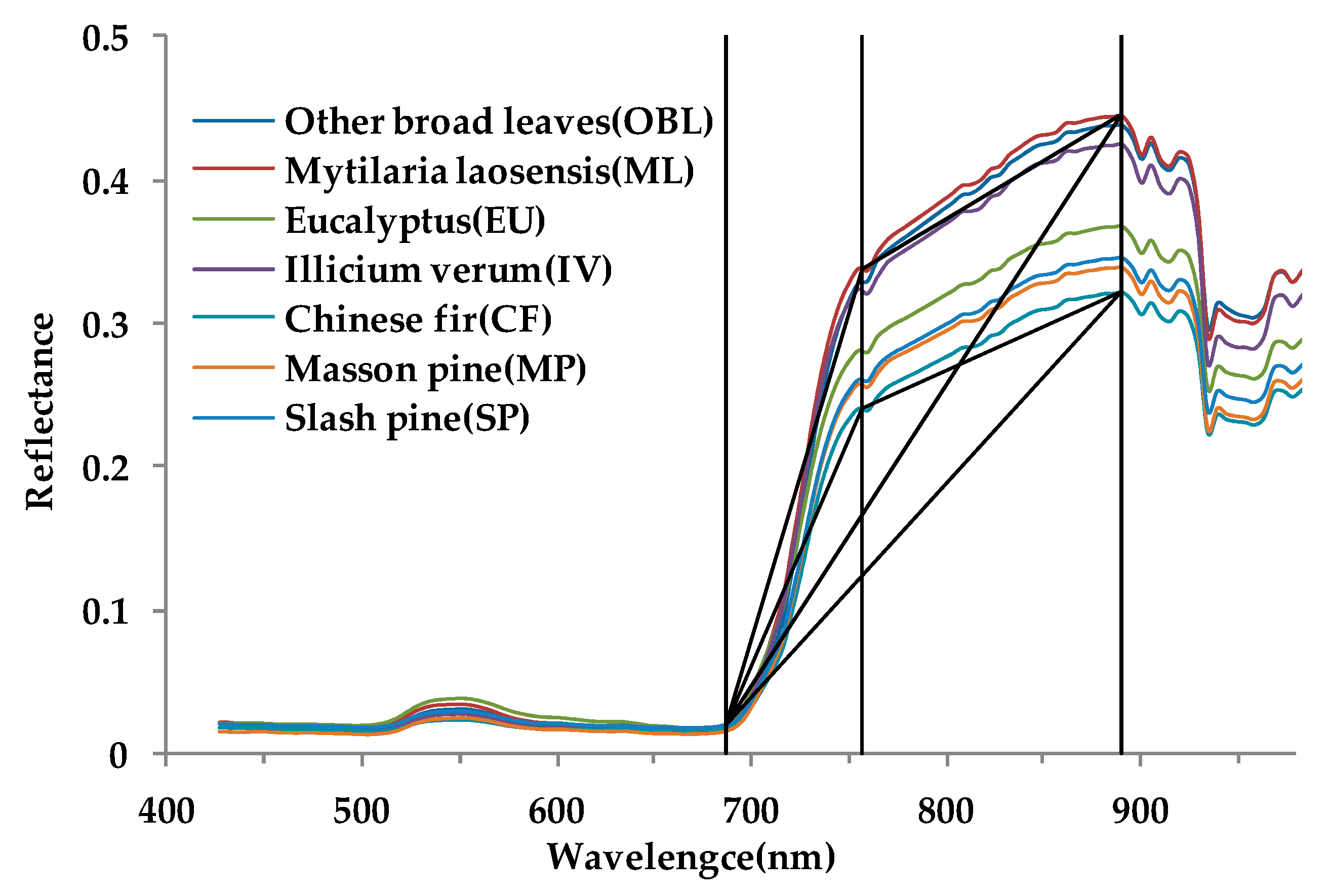
Slope between wavelengths 687 nm and 760 nm SL 1 Calculated as Equation (1)
Slope between wavelengths 687 nm and 890 nm   SL 2 Calculated as Equation (2)
Triangle area enclosed by wavelengths 687 nm, 760 nm and 890 nm TA Calculated as Equation (3)
Note: The hyperspectral image spectral band is   ρ and the wavelength is 400 nm to 1000 nm.
Table 5. Extracted four sets of feature variables for classification.
FeaturesDescription
Independent components analysisThe first five ICA transformation images.
Spectral indexNine vegetation indices, including NDVI, PSRI, MRESRI, MRENDVI, GNDVI, PRI, SIPI, ARI1, VOG1, and three new constructed spectral indices, including SL1, SL2 and TA.
Textural featuresSelected 17 × 17 texture window size extracted 24 textural features, including MEAN, VAR, HOM, CON, DIS, ENT, SM, COR calculated using GLCM with three bands (band 482 nm, band 550 nm and band 650 nm).
Canopy height modelCanopy height model obtained by LiDAR data, reflected the height information of each tree species.
Table 6. The schemes carried out in this study using the k-nearest neighbor (KNN) and support vector machine (SVM) classifiers.
SchemesFeature Variables
Scheme AThe first five ICA transformation images, ICA1-ICA5.
Scheme BThe first five ICA transformation images stacking 13 spectral indices.
Scheme CThe feature variables in Scheme B stacking 24 textural features.
Scheme DAll feature variables stacking together, including the first five ICA transformation images, spectral indices, textural features, and CHM.
Scheme EFeatures selected by RF, including four independent components, i.e., ICA2, ICA3, ICA4, ICA5, seven spectral index features, i.e., NDVI, PRI, GNDVI, PSRI, SL2, SIPI and ARI1, six texture features, i.e., HOM_G550, ENT_G550, CON_G550, COR_G550, DIS_R650, SM_R650, and CHM.
Scheme FFeatures selected by SVM-RFE, including four independent components, i.e., ICA2, ICA3, ICA4, ICA5, five spectral index features, i.e., NDVI, PRI, GNDVI, SL2, and PSRI, eight texture features, i.e., HOM_G550, Mean_G550, DIS_G550, VAR_G550, CON_G550, ENT_G550, ENT_R650, VAR_R650, and CHM.
Table 7. The overall accuracy of different classification schemes using the KNN and SVM classifiers.
SchemesKNNSVM
Overall Accuracy (OA)Kappa CoefficientOverall Accuracy (OA)Kappa Coefficient
Scheme A80.51%0.76783.08%0.798
Scheme B84.25%0.81286.25%0.836
Scheme C87.11%0.84690.86%0.891
Scheme D90.28%0.88493.26%0.920
Scheme E89.42%0.87494.14%0.930
Scheme F89.86%0.87994.68%0.937
Note: The numbers with gray background in this table indicate the highest classification accuracy corresponding to different classifiers.
Table 8. Species classification accuracy with the KNN classifier for different classification schemes.
Tree SpeciesScheme AScheme BScheme CScheme DScheme EScheme F
PAUAPAUAPAUAPAUAPAUAPAUA
IV80.5074.5085.9179.5187.3183.9385.4589.1884.8388.3984.3787.62
EU93.9189.8096.2391.3993.9193.9896.2395.0995.7595.9097.2795.74
ML81.2586.2283.3381.1290.5486.1392.7992.3491.3592.5394.8792.21
CF83.6279.2587.4185.9390.1790.3388.2896.0692.2492.5688.1096.05
MP81.2677.0986.1382.2787.2184.4793.3385.4893.3383.6894.4183.31
SP62.0972.6281.1780.5690.0881.0190.3384.5284.9985.2085.2487.24
OBL64.3071.7961.3679.9768.7281.5981.6884.1678.4881.1978.4881.87
Note: The numbers with gray background in this table indicate the highest producer accuracy of each tree species. Tree species are abbreviated as follows: IV, Illicium verum; EU, eucalyptus; ML, mytilaria laosensis; CF, Chinese fir; MP, masson pine; SP, slash pine; OBL, other broad leaves. Other abbreviations in the table: PA, producer accuracy (%) and UA, user accuracy (%).
Table 9. Species classification accuracy with the SVM classifier for different classification schemes.
Tree SpeciesScheme AScheme BScheme CScheme DScheme EScheme F
PAUAPAUAPAUAPAUAPAUAPAUA
IV86.3874.8086.8482.6291.0287.2497.0395.8097.4396.0596.0797.88
EU95.2791.9593.5093.0696.2395.7794.3992.0390.7189.8489.1792.64
ML82.3790.6588.4682.2790.5492.1786.6999.4790.6991.9696.9587.79
CF88.6282.3787.2491.0190.5292.4310083.8097.3799.3791.1990.89
MP83.0675.7087.2183.5910087.8290.8691.6596.4492.8995.67100
SP71.2583.5890.0880.8293.1382.6293.8791.8992.7990.1910095.20
OBL62.4375.3268.3282.8274.3391.1589.5793.5891.1895.5294.8393.54
Note: The numbers with gray background in this table indicate the highest producer accuracy of each tree species. Tree species are abbreviated as follows: IV, Illicium verum; EU, eucalyptus; ML, mytilaria laosensis; CF, Chinese fi; MP, masson pine; SP, slash pine; OBL, other broad leaves. Other abbreviations in the table: PA, producer accuracy (%) and UA, user accuracy (%).

