Estimation of Pinus massoniana Leaf Area Using Terrestrial Laser Scanning

Abstract

The accurate estimation of leaf area is of great importance for the acquisition of information on the forest canopy structure. Currently, direct harvesting is used to obtain leaf area; however, it is difficult to quickly and effectively extract the leaf area of a forest. Although remote sensing technology can obtain leaf area by using a wide range of leaf area estimates, such technology cannot accurately estimate leaf area at small spatial scales. The purpose of this study is to examine the use of terrestrial laser scanning data to achieve a fast, accurate, and non-destructive estimation of individual tree leaf area. We use terrestrial laser scanning data to obtain 3D point cloud data for individual tree canopies of Pinus massoniana. Using voxel conversion, we develop a model for the number of voxels and canopy leaf area and then apply it to the 3D data. The results show significant positive correlations between reference leaf area and mass (R² = 0.8603; p < 0.01). Our findings demonstrate that using terrestrial laser point cloud data with a layer thickness of 0.1 m and voxel size of 0.05 m can effectively improve leaf area estimations. We verify the suitability of the voxel-based method for estimating the leaf area of P. massoniana and confirmed the effectiveness of this non-destructive method.

1. Introduction

As an important organ of trees, leaves play a substantial role in plant photosynthesis, transpiration, and many other physiological activities [1,2,3]. The leaf area (LA) is an important parameter for expressing the amount of leaves in a tree canopy, and is an important measurement for understanding the growth, development, productivity, and physiology of plants [4,5]. Evaluations of leaf traits at the leaf are receiving more attention in forest ecology and remote sensing studies [6,7], LA directly affects the accumulation of plant dry matter and also directly determines the interception capacity and utilization rate of light energy, as well as changes in transpiration rates. Another indicator related to LA is the specific leaf area (SLA), which refers to the fresh leaf surface area per unit mass of dry matter; its value is directly affected by leaf thickness, shape, and quality. Many ecosystem process models utilize plant SLA as an important input parameter [8]. Therefore, rapid and non-destructive acquisition of parameters is very important for the estimation of the stand structure and the quantification of stand quality.

Currently, commonly used leaf area measurement methods include direct methods and indirect methods [9,10,11]. Many direct methods require the excision of leaves from plants; this method is labor-intensive and limited in the scope of its application. Indirect measurement methods primarily use a variety of instruments and software to obtain leaf area measurements, such as portable scanning planimeters, hand scanners, laser optic apparatuses, and image analysis software. LA can be obtained by a variety of instruments and software [12]. Most terrestrial laser scanners (TLSs) cannot separate branches and leaves directly. Methods using TLSs are also time consuming, expensive, complex, and only suitable for a few specific species of plants [13]. Especially when studying species with non-flattened blades (e.g., coniferous species, such as P. thunbergii and Pinus massoniana), such methods result in poor comparability, owing to differences in the understanding of principles of leaf interception [14]. Therefore, new instruments and methods to separate individual trees from the other trees must be explored [6,15].

Recently, many studies have estimated LA by terrestrial light detection and ranging (voxeli). LiDAR is an active remote sensing technology that records the details of three-dimensional information by acquiring the three-dimensional coordinate data and digital images of the research target [16], thereby providing an opportunity to extract the 3D geometry of an individual tree. The estimation of tree characteristics such as height and diameter at breast height (DBH), has been widely used to fully compensate for the limitations of traditional optical remote sensing monitoring in the vertical structure of forest canopy [17,18]. TLSs are also used in measuring vegetation structure information. TLSs are lightweight and portable, have high laser resolution and are safe. Most TLSs use a level 1 laser, which does not harm the human eye. The tree canopy structure is quickly and accurately measured by a pulsed laser in a non-contact manner, thereby obtaining a large-area, complex, irregular forest point cloud data [19,20]. Another advantage of TLSs is their capability to separate a target tree from other trees using its unique distance information. There are three methods for estimating the leaf area of individual trees: regression analysis, gap-based probability, and voxel method.

Regression analysis is mainly based on TLSs to obtain structural parameters of a single tree—such as crown width, breast diameter, tree height—to establish a regression equation of the leaf area [21]. This method is more labor-saving than field measurement and is conducive to data preservation and extraction. There is an error in the extraction process of the forest structure parameters, and this error tends to have an uncertain effect on the subsequent regression equations.

Based on the gap probability and the law of angular distribution, the LAI of the individual tree is derived, and the influence of the relevant parameters on the LAI estimation is analyzed [22], but the trunk effect in the interference probability model is not eliminated.

The voxel-based 3D modeling method has been used for years in the fields of scientific computation and medical imaging. This method is convenient for creating architectural models and for 3D imaging. It is, in fact, a method based on regression models. In forestry research, voxel-based 3D modeling is used to estimate LAI and leaf area density (LAD) by directly counting the contact frequency of each layer of the studied tree [23,24]. However, this method is primarily applied to broad-leaved tree species, and further study is required to adapt this method to conifer species and obtain the leaf areas of conifer needles.

Masson’s pine (Pinus massoniana Lamb.) is one of the most important tree species in southern China. Because of its high adaptability to drought and barren soils and its capacity to retain water and nutrients, P. massoniana has been widely planted in China [25,26]. LA usually represents the quality of a tree [27,28,29]. However, because of the non-flattened blades of P. massoniana, such methods result in poor comparability, owing to differences in the understanding of principles of leaf interception [14].

This study combines different horizontal layers and different voxel sizes to estimate the LA of P. massoniana based on the 3D voxel method. Here, ‘horizontal layer’ indicates the bottom layer of the canopy. The purpose of this study was to: (1) construct a conifer tree LA estimation method based on ground-based remote sensing data; (2) study the optimal voxel size and model in the LA estimation process; and (3) study the LA estimation under the optimal stratification height.

2. Materials and Methods

Figure 1 illustrates the developed LA estimation workflow, including the extraction of the reference LA and the estimation of the LA. The specific steps are as follows:

2.1. Site Characteristics

This study site was located in Hetian Town (25°33′–25°48′ N, 116°18′–116°31′ E), in Fujian Province, China. The site is dominated by P. massoniana plantations. The site is characterized by low hills and the average elevation is ~310 m above sea level [30]. The mean annual air temperature is 19 °C, and the annual precipitation is 1621 mm (occurs mainly from April to June) [31].

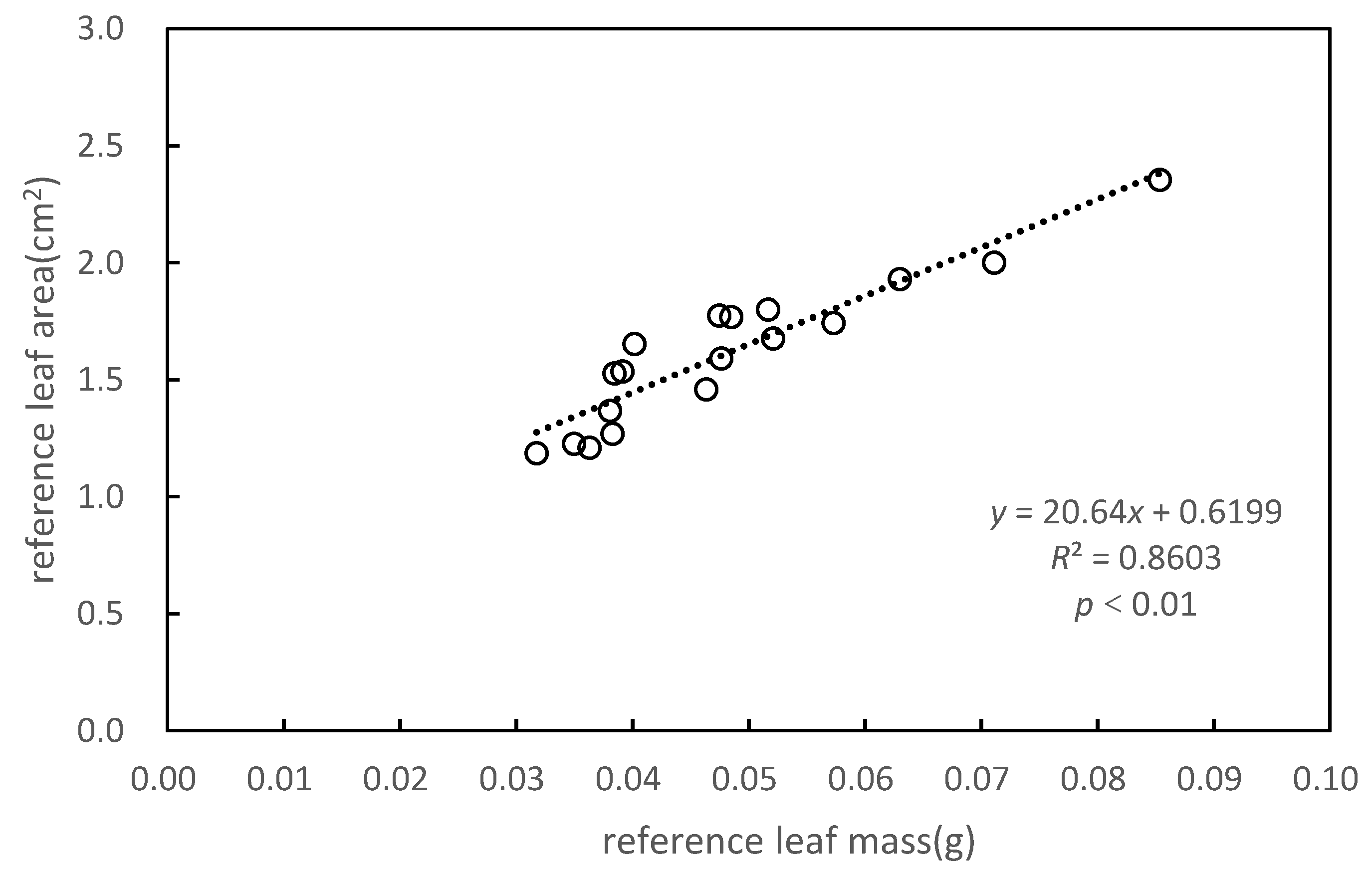
2.2. Specific Leaf Area Acquisition

A total of 26 canopy samples of P. massoniana were selected for sampling. Samples of 10 needles, with no signs of disease and of the same color, were collected from the upper, middle, and lower layers of the canopy. We first used the YMJ-C Digital Leaf Area Meter (HINOTEK, Hangzhou City, China) system to scan the coniferous area, and then loaded the needles into numbered envelopes and brought them back to the laboratory to dry to a constant weight. Then, each sample was weighed and a single mean dry weight was calculated [32]. The specific leaf area of P. massoniana was obtained by the least-squares method [4].

$$\mathrm{SLA}=\frac{{{\displaystyle \sum }}_{i=1}^n{LA}_i{\ast X}_i}{{{\displaystyle \sum }}_{i=1}^n{X}_i{}^2}$$

(1)

where n is the number of leaves tested, LA_i is the leaf area of the ith leaf, and X_i is the dry mass of the ith leaf.

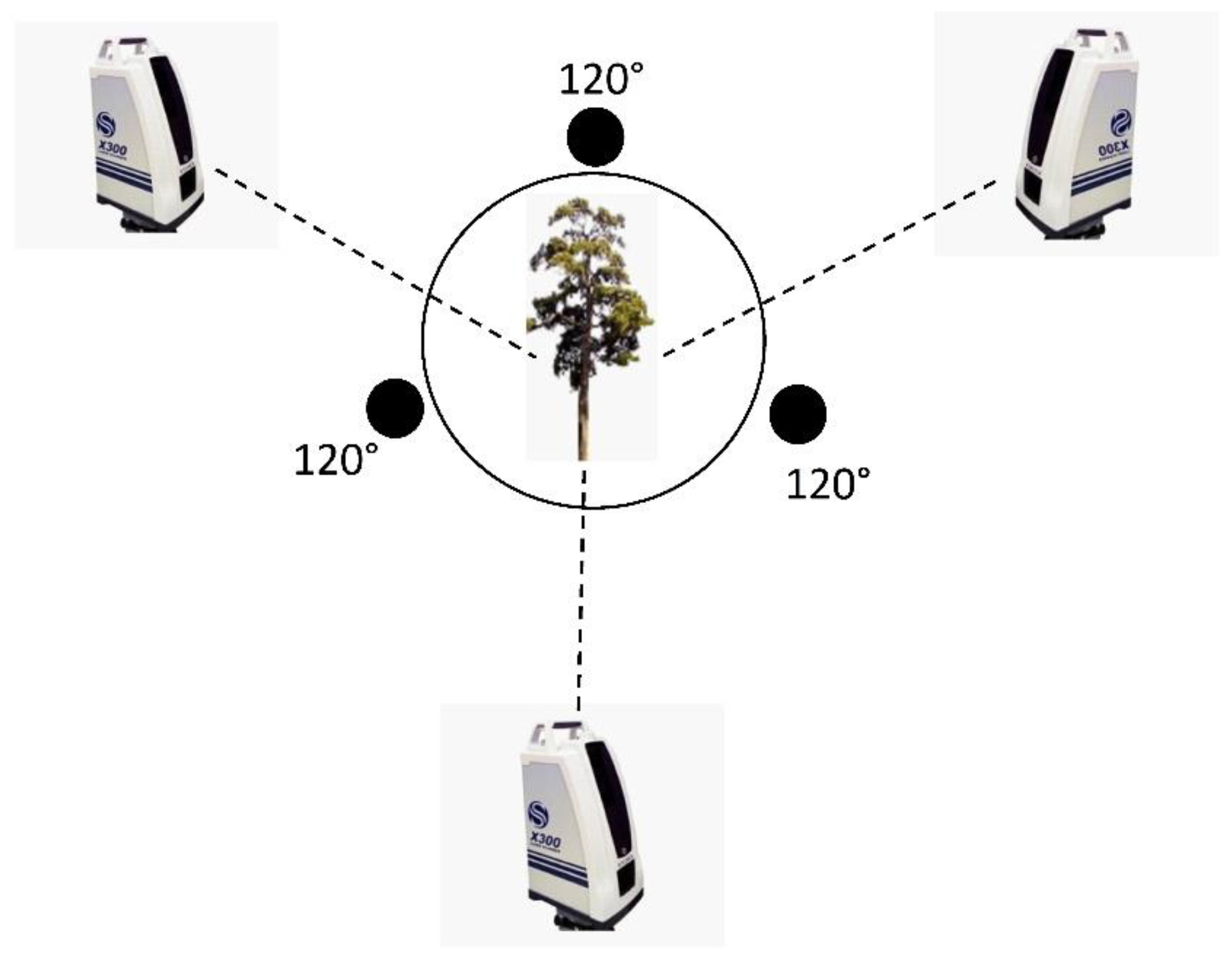
2.3. Point Cloud Data Acquisition

We obtained point cloud data for 26 P. massoniana samples using a Stonex X300 laser scanner (Italy), which is a pulsed-static 3D laser scanner. The configuration of the Stonex X300 is shown in

Table 1. Configuration of the STONEX X300 laser scanner

Model	STONEX X300
Measuring range	2–300 m (100% Reflectivity)
Visual range	Level 360° (Panoramic view) vertical 90° (−25° to +65°)
Accuracy	<6 mm (50 m) <40 mm (300 m)
Scanning speed	>40,000 points/s
Scan resolution	0.37 mrad
Data storage	32 GB

. In order to avoid the influence of light intensity and weather on measurement error, we selected three different angles (Figure 2) [23], corresponding to (1) an instrument shooting angle of 220°, (2) a scanning mode set to fast, and (3) a horizontal field of view of the scanning area with partial station overlap, such that any two stations could be found between multiple points of the same name with a vertical field of view of −25° to 65°. The scan resolution accuracy was <6 mm. Three plastic balls, with a diameter of 20 cm each, were placed next to each sample tree and on the top of a tripod to serve as a fixed target, ensuring that each station could scan at least two targets and match the three stations through the target using the original point cloud data.

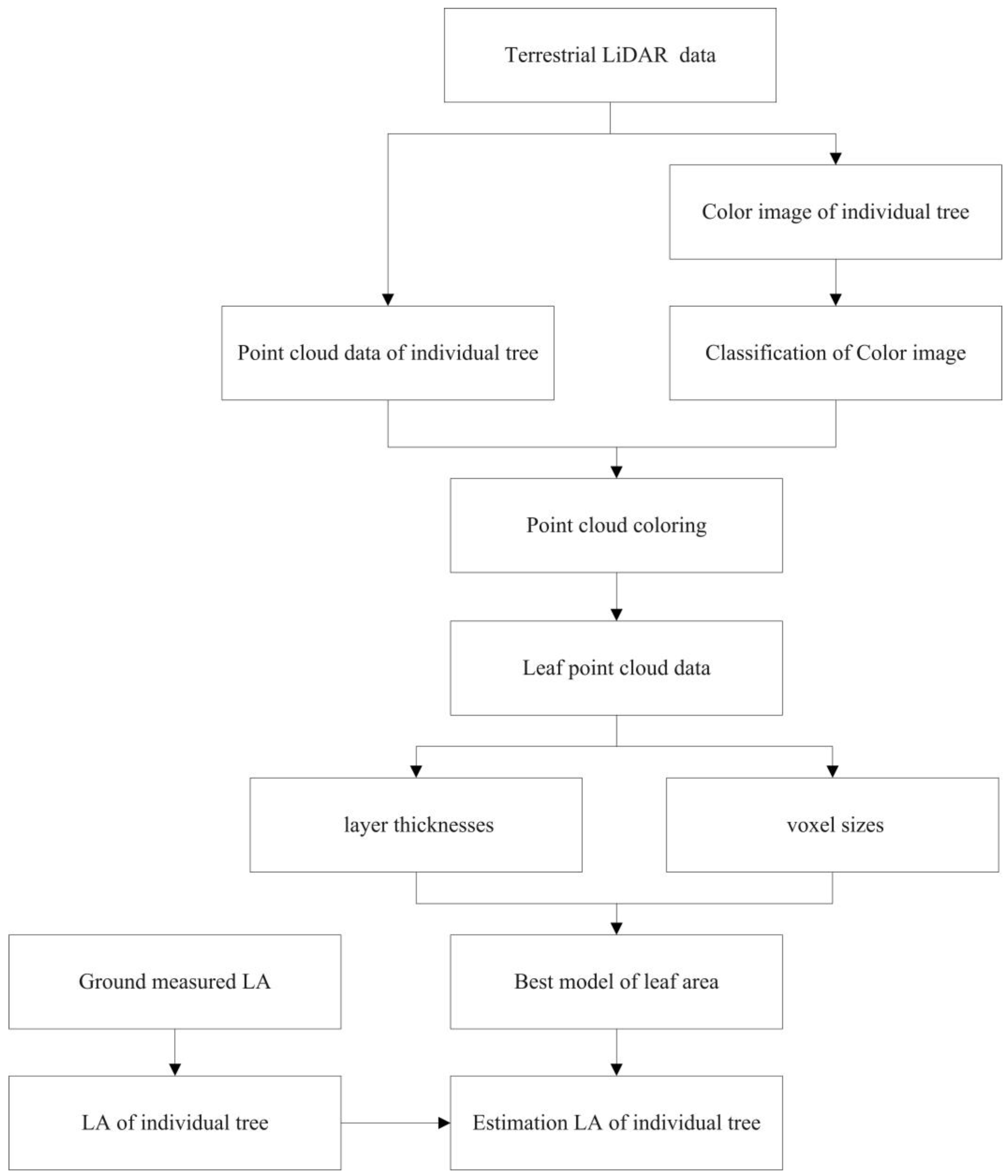
2.4. Point Cloud Data Processing

In this study, the area of each layer was calculated according to the edge length, L. Choosing a suitable voxel size solved the difference in the number of point clouds in voxels:

$$\{\begin{array}{c}a=x_{min}+\left(\frac{int\left(x-x_{min}\right)}{L}\right)\times L\\ b=y_{min}+\left(\frac{int\left(y-y_{min}\right)}{L}\right)\times L\\ c=z_{min}+\left(\frac{int\left(z-z_{min}\right)}{L}\right)\times L\end{array}$$

(2)

where a, b, and c are the coordinates in the voxel array, int is a function for rounding off the coordinates to one decimal place to the nearest integer; x, y, and z represent the point coordinates of the registered LiDAR data; x_min, y_min, and z_min are the minimum values of x, y, and z, and L represents the voxel element size [33,34]. In this article, the voxel type selected is the filled voxels that contain a group of points [35,36].

First, we layered the point cloud data according to different layer thicknesses and subsequently calculated the number of voxels under different layer thicknesses. Through layering treatment, the overlap between the blades was effectively reduced, so that the number of transformed voxels was more representative of the blade area. The rounding algorithm is shown in Figure 3.

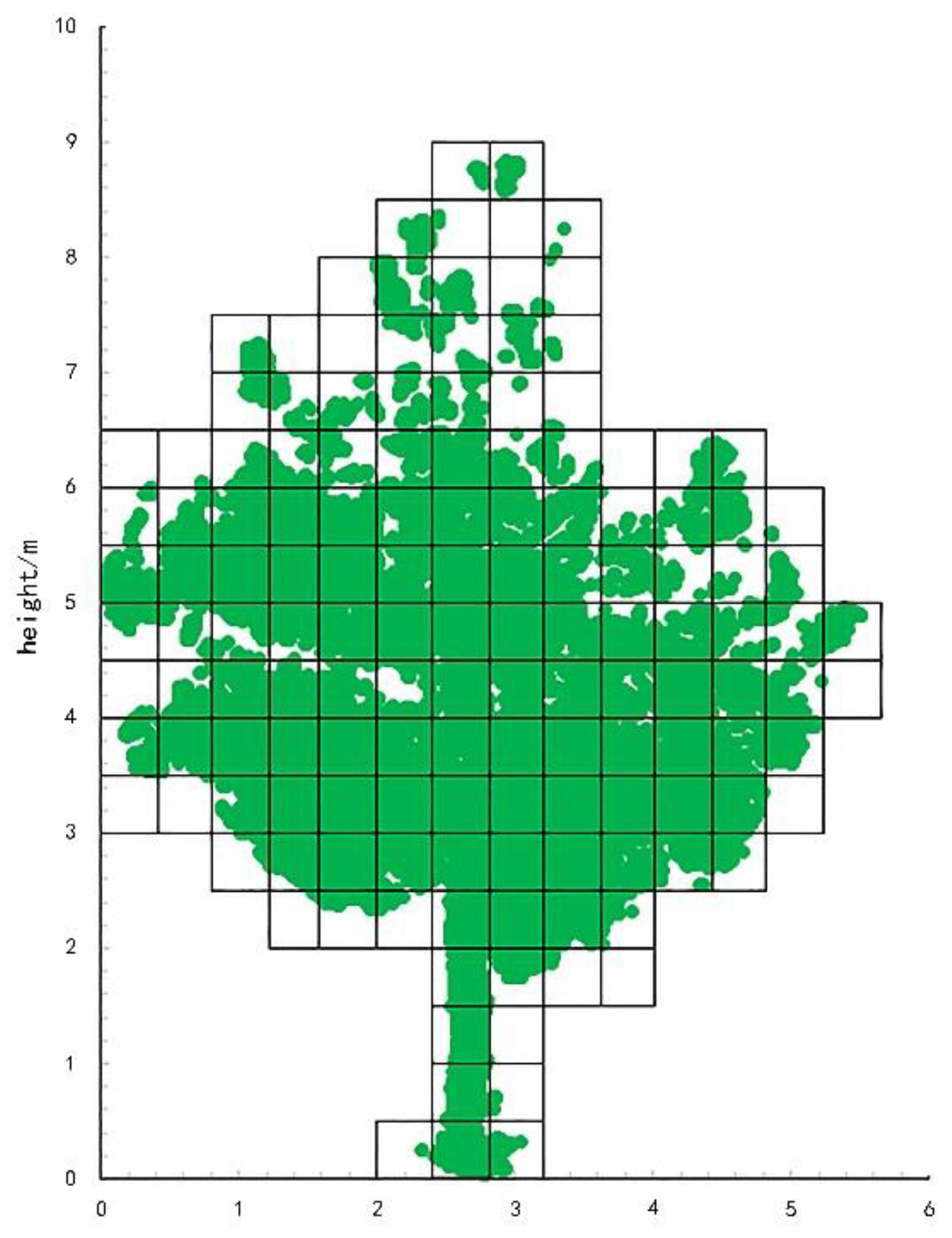
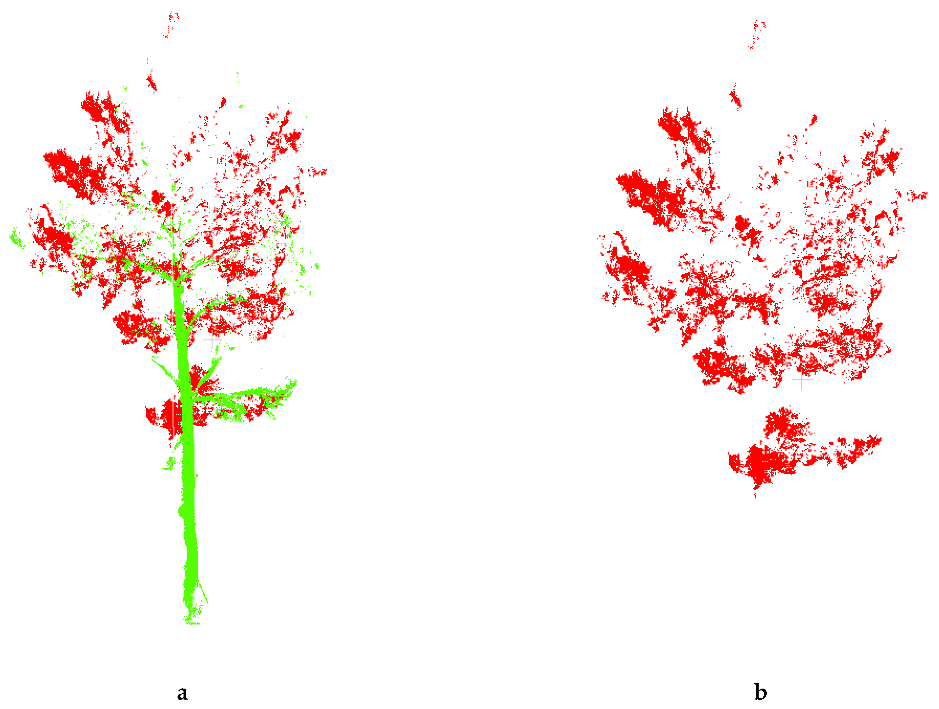
2.5. Point Cloud Data Extraction

Firstly, the original point cloud data obtained by TLS Stonex X300 is used to convert the original point cloud data, and the true color photos are extracted. The leaves, branches and other selections in the original color image are used as training samples to unify other training samples, and then use the maximum likelihood method to classify the image. In order to make the color clear after classification, this article sets the canopy leaves to red, the branches and trunks to green, and the other training samples to white (Figure 4).

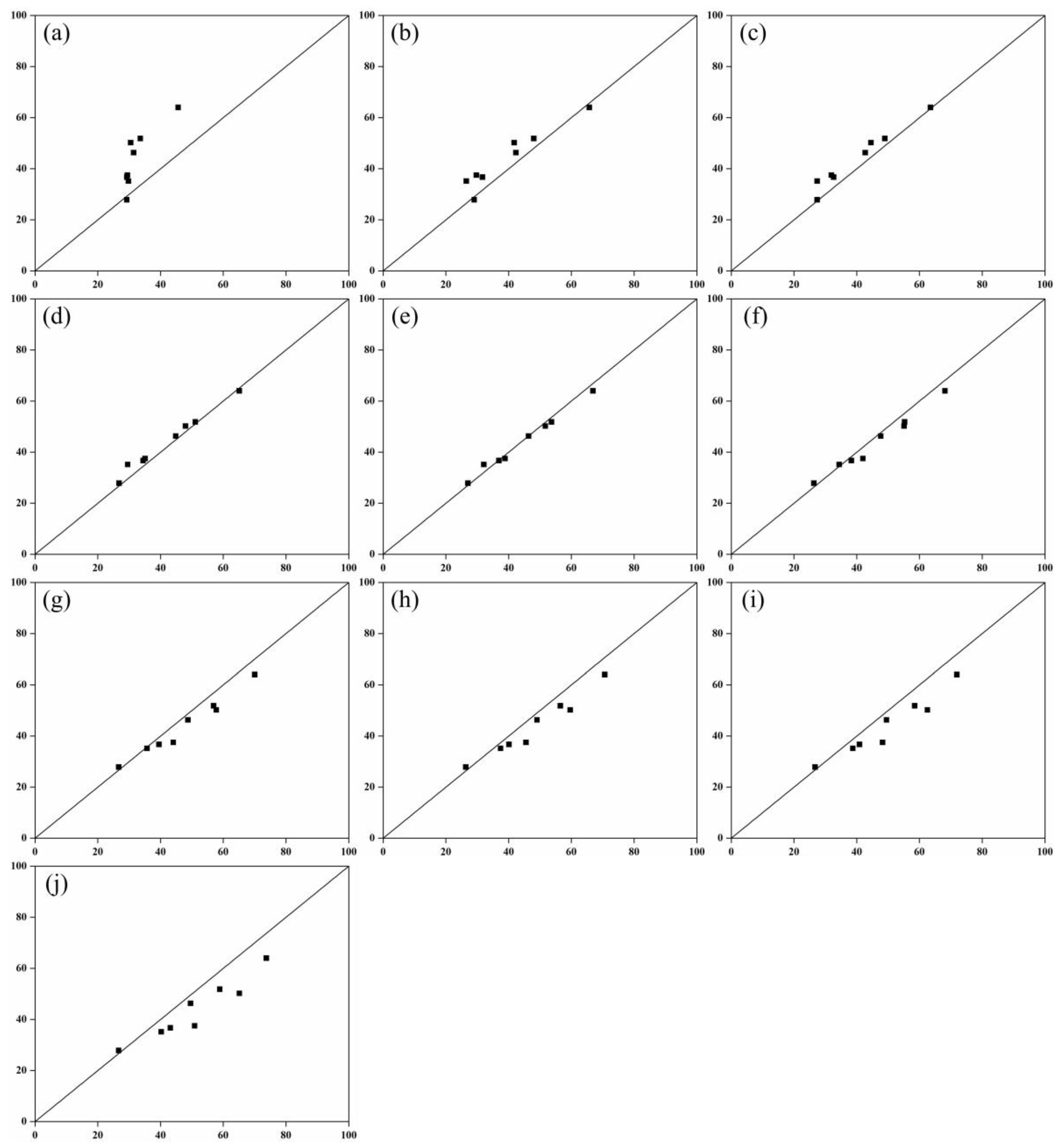
2.6. Model Validation

In order to develop models, the data from 26 individual trees were first classified into two independent subsets for model establishment and model validation. A subset of 18 individual trees was used for model establishment, and the data of five individual trees were used for model validation. With the subset of 18 individual trees used for modelling, the correlations between leaf area and leaf mass were first analyzed, and then single-variable models were established. Single-variable models contained linear, quadratic, and exponential forms, using each of the 10 layer and 10 voxel sizes. The models were validated according to the root mean square error (RMSE) and mean relative error (MRE) using Equations (3) and (4), respectively:

$$\mathit{RMSE}={\left(\frac{1}{n}{{\displaystyle \sum }}_{i=1}^n{\left(E_i-M_i\right)}^2\right)}^{\frac{1}{2}}$$

(3)

$$\mathit{MRE}=\frac{1}{n}{{\displaystyle \sum }}_{i=1}^n\frac{{}_{\mathrm{abs}}\left(E_i-M_i\right)}{M_i}\times 100\%$$

(4)

Statistical analyses were performed using SPSS version 12.0 (Amos Development Corporation, Chicago, IL, USA).

3. Results

3.1. Specific Leaf Area of Pinus massoniana

The dataset was divided into training data and test data by the random selection of 30% of the total data set as testing data and 70% as training data. The reference leaf mass, reference LA, and SLA of the training data are shown in

Table 2. Leaf parameters

Sample Number
	1-1	1-2	1-3	1-4	1-5	1-6	1-7	1-8	1-9
Reference leaf mass (g)	0.038	0.057	0.032	0.071	0.038	0.046	0.048	0.038	0.052
Reference leaf area (cm2)	1.528	1.743	1.187	2.002	1.269	1.459	1.592	1.367	1.800
SLA (cm2/g)	39.705	30.397	37.390	28.142	33.130	31.463	33.394	35.891	34.810
	2-1	2-2	2-3	2-4	2-5	2-6	2-7	2-8	2-9
Reference leaf mass (g)	0.049	0.035	0.039	0.085	0.063	0.040	0.052	0.036	0.047
Reference leaf area (cm2)	1.769	1.226	1.535	2.354	1.930	1.653	1.677	1.209	1.774
SLA (cm2/g)	36.464	35.035	39.196	27.570	30.623	41.159	32.169	33.268	37.365

Abbreviations: Specific leaf area, SLA.

. The reference values for leaf mass and LA were obtained as the average of 10 values. The correlations between the reference leaf mass and the reference LA are shown in Figure 5.

To obtain a more accurate LAI, we calculated the LA of individual trees based on the SLAs of the upper, middle, and lower parts of P. massoniana (Figure 5). Significant correlations were found between reference LA and reference leaf mass, with a coefficient of determination (R²) of 0.8603. LA was positively correlated to leaf mass (p < 0.01). The SLA of P. massoniana was obtained by the least-squares method (Table 1).

SLA may be affected by light, temperature, nutritional status, leaf age, and other factors. It can be seen that the average dry weight of P. massoniana did not differ much, but the difference in the dry weight of leaves with different leaf ages was larger, indicating that there is a certain difference in dry matter accumulation between new leaves and old leaves. Among these, the maximum LA was 2.354 (sample 2-4), the minimum LA was 1.187 (sample 1-3), the maximum leaf mass was 0.085 (sample 2-4), and the minimum LA was 0.032 (sample 1-3). The maximum SLA was 41.159 (sample 2-6) and the minimum SLA was 27.57 (sample 2-4).

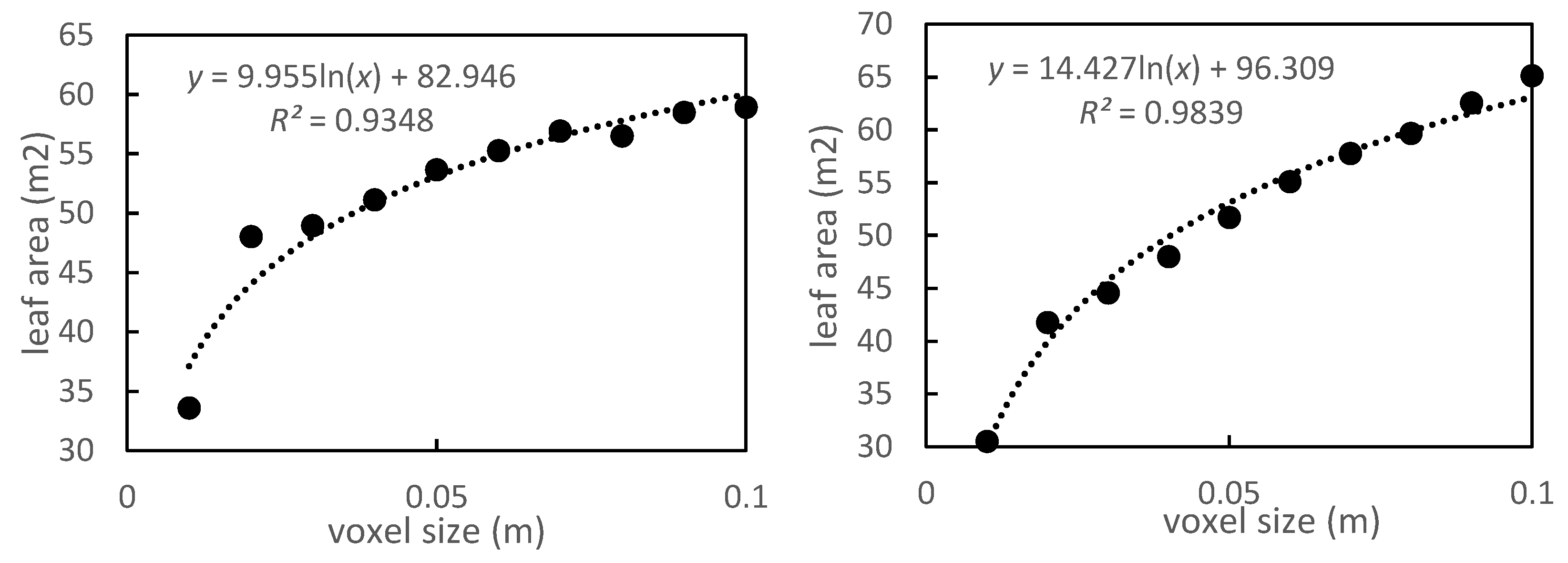
3.2. Leaf Area Estimation at Different Scales

In order to reduce the influence of terrain and scanning distance on the data volume of point clouds in the process of using 3D laser scanners in the field, and to establish a more accurate relationship between point cloud data and LA, a voxel conversion method was adopted in this study based on different voxel size to establish a LA estimation model. Based on the subset of 18 data points, a total of 300 single-variable models were established for each of the 10 needle types, and the R² values of these models are shown in

Table 3. Coefficient of determination (R²) for LA estimates.

R2 of Different Scales of LA Estimation
Layers (m)	0.1	0.2	0.3	0.4	0.5	0.6	0.7	0.8	0.9	1
0.01 (m)
L	0.532	0.575	0.59	0.594	0.603	0.603	0.606	0.609	0.61	0.63
E	0.4	0.428	0.44	0.444	0.454	0.452	0.457	0.459	0.459	0.481
Q	0.649	0.654	0.659	0.659	0.661	0.662	0.661	0.663	0.662	0.673
0.02 (m)
L	0.652	0.686	0.707	0.71	0.717	0.72	0.723	0.727	0.729	0.753
E	0.497	0.528	0.548	0.551	0.561	0.561	0.569	0.57	0.571	0.599
Q	0.69	0.71	0.725	0.728	0.732	0.735	0.736	0.74	0.74	0.761
0.03 (m)
L	0.708	0.746	0.765	0.768	0.773	0.777	0.781	0.782	0.786	0.809
E	0.548	0.586	0.606	0.61	0.62	0.622	0.631	0.629	0.631	0.662
Q	0.729	0.757	0.773	0.776	0.781	0.785	0.787	0.788	0.791	0.812
0.04 (m)
L	0.749	0.785	0.804	0.806	0.611	0.817	0.821	0.817	0.823	0.844
E	0.587	0.625	0.646	0.652	0.662	0.665	0.676	0.67	0.673	0.703
Q	0.76	0.79	0.807	0.809	0.815	0.82	0.824	0.82	0.825	0.845
0.05 (m)
L	0.755	0.793	0.81	0.812	0.832	0.838	0.841	0.836	0.844	0.847
E	0.583	0.624	0.645	0.647	0.691	0.693	0.704	0.698	0.701	0.715
Q	0.767	0.798	0.813	0.814	0.835	0.84	0.843	0.839	0.845	0.849
0.06 (m)
L	0.8	0.831	0.844	0.844	0.847	0.854	0.847	0.845	0.859	0.871
E	0.641	0.68	0.7	0.702	0.712	0.716	0.705	0.706	0.723	0.749
Q	0.804	0.833	0.846	0.846	0.849	0.856	0.848	0.847	0.86	0.87
0.07 (m)
L	0.815	0.845	0.857	0.856	0.857	0.862	0.865	0.858	0.865	0.877
E	0.659	0.698	0.715	0.718	0.728	0.732	0.742	0.733	0.735	0.763
Q	0.819	0.847	0.858	0.857	0.858	0.864	0.866	0.86	0.866	0.878
0.08 (m)
L	0.834	0.851	0.869	0.865	0.868	0.873	0.876	0.869	0.877	0.886
E	0.681	0.706	0.732	0.732	0.747	0.749	0.762	0.75	0.75	0.779
Q	0.837	0.852	0.87	0.866	0.869	0.875	0.877	0.871	0.878	0.886
0.09 (m)
L	0.82	0.862	0.871	0.868	0.868	0.873	0.873	0.868	0.876	0.878
E	0.689	0.722	0.741	0.74	0.75	0.755	0.764	0.755	0.757	0.778
Q	0.829	0.863	0.872	0.869	0.869	0.875	0.874	0.869	0.877	0.878
0.1 (m)
L	0.859	0.87	0.875	0.873	0.873	0.881	0.878	0.829	0.879	0.881
E	0.71	0.738	0.761	0.755	0.764	0.768	0.775	0.739	0.764	0.788
Q	0.861	0.871	0.877	0.874	0.873	0.882	0.879	0.835	0.88	0.882

Model types: linear, L; exponential, E; quadratic, Q.

. The largest R² was for the quadratic model between 0.1 m and 0.08 m (R² = 0.886), the lowest was for the exponential model between 0.1 m and 0.01 m (R² = 0.4), and the average of all single-variable models was R² = 0.757. The average R² values of each of the 75 single-variable models were ranked as: quadratic (0.811) > linear (0.799) > exponential (0.661). As for the layered levels, the average R² increased with increasing layer thickness, as 1 m (0.788) > 0.9 m (0.771) > 0.8 m (0.763) > 0.7 m (0.77) > 0.6 m (0.767) > 0.5 m (0.756) > 0.4 m (0.755) > 0.3 m (0.754) > 0.2 m (0.738) > 0.1 m (0.709). It is notable that the average R² of the models based on 0.01 m was the lowest. This indicates that the voxel value was too small to reduce the influence of the 3D laser scanning distance on the point cloud density. A ‘best’ single-variable model was selected for each of the layer types and voxel sizes according to the R² values and model stabilities (Table 3). The independent variables of these selected models contained 10 voxel sizes for different layers, and most were quadratic.

3.3. Model Validation

Using the 10 selected models (Equations (5–14) in

Table 4. Selected single-variable models for estimating LA.

Voxel	Model	R2
0.01	$\mathrm{y}=1\times {10}^{-8}{x}^2-0.0005x+35.498$	0.673
0.02	$\mathrm{y}=3\times {10}^{-8}{x}^2- 0.0009x+15.204$	0.761
0.03	$\mathrm{y}=4\times {10}^{-8}{x}^2-0.0024x+9.6254$	0.812
0.04	$\mathrm{y}=5\times {10}^{-8}{x}^2-0.0042x+6.4524$	0.845
0.05	$\mathrm{y}=1\times {10}^{-7}{x}^2-0.0055x+7.1991$	0.849
0.06	y = 0.0088x + 2.8488	0.871
0.07	$\mathrm{y}=2\times {10}^{-7}{x}^2-0.0093x+5.5129$	0.878
0.08	$\mathrm{y}=2\times {10}^{-7}{x}^2-0.0115x+4.8836$	0.886
0.09	$\mathrm{y}=3\times {10}^{-7}{x}^2-0.0133x+5.536$	0.878
0.1	$\mathrm{y}=4\times {10}^{-7}{x}^2-0.0156x+5.2663$	0.882

Note: y = leaf area; x = number of voxels.

), LA were calculated for different voxel sizes with the eight sets of independent validation data. For the 10 voxel sizes, the maximum, minimum, and mean RMSE of the multivariate models were 13.36, 1.94, and 5.75 (Figure 6), respectively. At first, as the scale factor increased, and the scatterplot of the model was more closely distributed along the 1:1 line (Figure 7). When the scale factor was greater than 0.5, the scatterplot of the model was more sparsely distributed along the 1:1 line. Among the 100 models established, the voxel size of 0.05 models for the 10 types performed best (i.e., the models based on a layer thickness of 1 m performed better than those based on a layer thickness from one radiometric correction image). This indicates that the ability to utilize 3D laser point cloud data is well-grounded at a layer thickness of 0.1 m and a voxel size of 0.05 to improve LA estimation [23].

4. Discussion

4.1. Measurement of Specific Leaf Area

Using leaf length and leaf width to establish LA is not feasible, and there are better measurements using leaf weight [37,38]. Furthermore, it is found that the blade quality has a better correlation with the blade area [19,39]. In order to improve the efficiency and obtain a more accurate canopy LA, a method of partially replacing the whole had been used in this study, and the canopy is divided into upper, middle, and lower parts to collect leaves. To ensure the consistency of the canopy structure and reduce the scanning error of the terrestrial LiDAR to the height of different canopy layers of P. massoniana, the P. massoniana canopy was divided into upper, middle, and lower parts, and the LA of each layer was calculated and subsequently used as the overall LA. However, the obtained leaf mass and LA still contain errors (Figure 5). This is due to the peculiarity of the leaf of the needle of the P. massoniana, and it is impossible to accurately measure the LA [12]. Significant correlations were found between the reference LA and reference leaf mass (Figure 1) [39,40,41]. We found that this rule also applies to P. massoniana (R² = 0.8603). The SLA of P. massoniana was obtained by the least-squares method. Based on the prediction of a linear model, estimates of LA and leaf quality [42] have been obtained, and the correlation is very high, suggesting that the model is still applicable to the LA of P. massoniana. Compared with the new leaves, the organic matter of the old leaves is more developed, and old leaves exhibit a higher dry matter content, with smaller LA [39,40].

4.2. Effects of Different Voxel Sizes

There is a clear linear relationship between LA and leaf mass. Many researchers have developed multiple regression models based on leaf width and leaf length [37,43]. However, the LA acquisition of P. massoniana remains very difficult. Therefore, in this study, TLSs were selected to estimate the leaf area of P. massoniana. In order to improve the spatial coverage and lessen the effects of occlusion, complete point cloud data were obtained by multiple scans. However, moving TLS parts (including supporting bases and reference targets) for multiple scans is labor-intensive and time consuming. Different scanning distances produce different numbers of point cloud data. The closer the scanning distance is, the larger the number of generated point cloud data becomes. Due to the influence of terrain and trees, it is often impossible to ensure the TLS scanning distance in the field. Therefore, we selected the voxel method to convert point cloud into voxel to improve the accuracy of leaf area estimation [44].

Different voxel sizes may affect the estimation of LA. The estimated LA was positively related to the voxel size, which was also related to the algorithm operating efficiency [34]. The smaller the voxel is, the larger the number of data is, and the slower the calculation becomes. If the voxel size is too large, there will be many blanks in the process of converting the point cloud into voxels. These blanks can then be calculated as the leaf area, increasing the estimated LA. The LA of P. massoniana increased with increase in voxel size. When the voxel value increases to 0.1 m, the estimated R² of the model reaches 0.886 (Table 4). The highest R² of the tree was 0.939. Therefore, choosing the appropriate voxel size was beneficial for reducing the leaf area estimation error. Our findings demonstrate that using terrestrial laser point cloud data with a layer thickness of 0.1 m and voxel size of 0.05 m effectively improved leaf area estimations [34,45].

Here, we show that a voxel value of 0.5 is ideal because it can reduce the impact of scanning distance on the establishment of a point cloud-LA model and can also avoid excessive calculations while providing optimal LA estimation results [25]. The purpose of voxelization is to reduce the influence of distance on the density of cloud points in the field during 3D scanning. If the voxel value is too small, it cannot reduce the impact of distance, and if it is too large, the point cloud density is too sparse, reducing the impact of point cloud density too much [46].

5. Conclusions

In this study, we investigated 26 P. massoniana trees. We determined the relationship between the number of voxels and LA, we used voxel size and layer thickness as the influencing factors for constructing the leaf area estimation model. The LA of P. massoniana was estimated and modeled, and the reference LA was used for model validation.

The results showed that it is feasible to extract P. massoniana LA based on terrestrial 3D laser techniques. Larger voxel values result in a greater delamination density and higher estimation accuracy. These findings highlight the feasibility of non-destructive acquisition of single LAs of P. massoniana based on TLS data. When the voxel value is 0.05, the optimal layer size is 1 m, and the best estimate model is the quadratic model. Using three stations for scanning, a complete canopy LA can be obtained and fully realized. Methods for estimation of LA are needed, and these findings will help develop and contribute to development of efficient TLS applications for forest inventories. In addition, the voxel-based 3D modeling method involves only a regression model. This study only applied the voxel-based modeling method to the estimation of the leaf area of P. massoniana. This method was not applied to other species It may only be effective for this species, and it can be used in future research of other species.

References

1. Chen, J.M.; Leblanc, S.G. A Four-scale bidirectional reflectance model based on canopy architecture. IEEE Trans. Geosci. Remote Sens. 1997, 35, 1316–1337. [Google Scholar] [CrossRef]
2. Sepaskhah, A.R.; Amini-Nejad, M.; Kamgar-Haghighi, A.A. Developing a dynamic yield and growth model for saffron under different irrigation regimes. Int. J. Plant Prod. 2013, 7, 473–504. [Google Scholar]
3. Shabani, A.; Sepaskhah, A.R.; Kamkar-Haghighi, A.A. A model to predict the dry matter and yield of rapeseed under salinity and deficit irrigation. Arch. Agron. Soil Sci. 2014, 61, 525–542. [Google Scholar] [CrossRef]
4. Diao, J.; Guo, H.; Lu, J.; Lei, X.D.; Tang, S.Z. Leaf area estimation model and specific leaf area of Chinese pine. For. Res. 2013, 26, 174–180. (In Chinese) [Google Scholar]
5. Baker, S.C.; Halpern, C.B.; Wardlaw, T.J.; Crawford, R.L.; Bigley, R.E.; Edgar, G.J.; Evans, S.A.; Franklin, J.F.; Jordan, G.J.; Karpievitch, Y.; et al. Short- and long-term benefits for forest biodiversity of retaining unlogged patches in harvested areas. For. Ecol. Manag. 2015, 353, 187–195. [Google Scholar] [CrossRef]
6. Weraduwage, S.M.; Chen, J.; Anozie, F.C.; Morales, A.; Weise, S.E.; Sharkey, T.D. The relationship between leaf area growth and biomass accumulation in Arabidopsis thaliana. Front. Plant Sci. 2015, 6, 167. [Google Scholar] [CrossRef] [PubMed]
7. Alton, P.B. The sensitivity of models of gross primary productivity to meteorological and leaf area forcing: A comparison between a Penman–Monteith ecophysiological approach and the MODIS Light-Use Efficiency algorithm. Agric. For. Meteorol. 2016, 218, 11–24. [Google Scholar] [CrossRef]
8. Landsberg, J.; Gower, S. Canopy Architecture and Microclimate. Appl. Physiol. Ecol. For. Manag. 1997, 51–88. [Google Scholar]
9. Sepaskhah, A.R. Estimation of individual and total leaf area of safflowers. Agron. J. 1977, 69, 783–785. [Google Scholar] [CrossRef]
10. Shabani, A.; Sepaskhah, A.R.; Kamkar-Haghighi, A.A. Growth and physiologic response of rapeseed (Brassica Napus L.) to deficit irrigation, water salinity and planting method. Int. J. Plant Prod. 2013, 7, 569–596. [Google Scholar]
11. Montero, F.; De Juan, J.; Cuesta, A.; Brasa, A. Nondestructive Methods to Estimate Leaf Area in (Vitis vinifera) L. HortScience 2000, 35, 696–698. [Google Scholar] [CrossRef]
12. Peksen, E. Non-destructive leaf area estimation model for faba bean (Vicia Faba L.). Sci. Hortic. 2007, 113, 322–328. [Google Scholar] [CrossRef]
13. Kandiannan, K.; Parthasarathy, U.; Krishnamurthy, K.S.; Thankamani, C.K.; Srinivasan, V. Modeling individual leaf area of ginger (Zingiber Officinale Roscoe) using leaf length and width. Sci. Hortic. 2009, 120, 532–537. [Google Scholar] [CrossRef]
14. Chen, J.M.; Black, T.A. Defining leaf area index for non-flat leaves. Plant Cell Environ. 1992, 15, 421–429. [Google Scholar] [CrossRef]
15. Salazar, J.C.S.; Melgarejo, L.M.; Bautista, E.H.D.; Di Rienzo, J.A.; Casanoves, F. Non-destructive estimation of the leaf weight and leaf area in cacao (Theobroma Cacao L.). Sci. Hortic. 2018, 229, 19–24. [Google Scholar] [CrossRef]
16. Wehr, A.; Lohr, U. Airborne laser scanning—An introduction and overview. ISPRS J. Photogramm. Remote Sens. 1999, 54, 68–82. [Google Scholar] [CrossRef]
17. Hese, S.; Lucht, W.; Schmullius, C.; Barnsley, M.J.; Dubayah, R.C.; Knorr, D.; Neumann, K.; Riedel, T.; Schroeter, K. Global biomass mapping for an improved understanding of the CO2 balance-the earth observation mission carbon-3D. Remote Sens. Env. 2005, 94, 94–104. [Google Scholar] [CrossRef]
18. Bouvier, M.; Durrieu, S.; Fournier, R.A.; Renaud, J.P. Generalizing predictive models of forest inventory attributes using an area-based approach with airborne LiDAR data. Remote Sens. Environ. 2015, 156, 322–334. [Google Scholar] [CrossRef]
19. Li, X.R.; Liu, Q.C.; Cai, Z. Specific leaf area and leaf area index of conifer plantations in Qianyanzhou station of subtropical china. J. Plant Ecol. 2007, 31, 93–101. (In Chinese) [Google Scholar]
20. Zhili, L.; Yu, Z.; Fengri, L.; Guangze, J. Non-destructively predicting leaf area, leaf mass and specific leaf area based on a linear mixed-effect model for broadleaf species. Ecol. Indic. 2017, 78, 340–350. [Google Scholar] [CrossRef]
21. Roberts, S.D.; Dean, T.J.; Evans, D.L.; McCombs, J.W.; Harrington, R.L.; Glass, P.A. Estimating individual tree leaf area in loblolly pine plantations using LiDAR-derived measurements of height and crown dimensions. For. Ecol. Manag. 2005, 213, 54–70. [Google Scholar] [CrossRef]
22. Bao, Y.; Ni, W.; Wang, D.; Yue, C.; He, H.; Verbeeck, H. Effects of Tree Trunks on Estimation of Clumping Index and LAI from HemiView and Terrestrial LiDAR. Forests 2018, 9, 144. [Google Scholar] [CrossRef]
23. Hosoi, F.; Omasa, K. Voxel-based 3-D modeling of individual trees for estimating leaf area density using high-resolution portable scanning LiDAR. IEEE Trans. Geosci. Remote Sens. 2006, 44, 3610–3618. [Google Scholar] [CrossRef]
24. Béland, M.; Baldocchi, D.D.; Widlowski, J.L.; Fournier, R.A.; Verstraete, M.M. On seeing the wood from the leaves and the role of voxel size in determining leaf area distribution of forests with terrestrial LiDAR. Agric. For. Meteorol. 2014, 184, 82–97. [Google Scholar] [CrossRef]
25. Yao, X.; Yu, K.; Deng, Y.; Zeng, Q.; Lai, Z.; Liu, J. Spatial distribution of soil organic carbon stocks in Masson pine (Pinus Massoniana) forests in subtropical China. Catena 2019, 178, 189–198. [Google Scholar] [CrossRef]
26. Ma, Z.; Hartmann, H.; Wang, H.; Li, Q.; Wang, Y.; Li, S. Carbon dynamics and stability between native Masson pine and exotic slash pine plantations in subtropical China. Eur. J. For. Res. 2014, 133, 307–321. [Google Scholar] [CrossRef]
27. Schaffer, B.; Schaffer, B.; Whiley, A.W.; Wolstenholme, B.N. The Avocado Botany, Production and Uses, 2nd ed.; Schaffer, B.A., Wolstenholme, B.N., Whiley, A.W., Eds.; CABI: Wallingford, UK, 2013. [Google Scholar]
28. Ghoreishi, M.; Hossini, Y.; Maftoon, M. Simple models for predicting leaf area of mango (Mangifera indica L.). J. Biol. Earth Sci. 2012, 2, 9. [Google Scholar]
29. McFadyen, L.M.; Morris, S.G.; Oldham, M.A.; Huett, D.O.; Meyers, N.M.; Wood, J.; McConchie, C.A.; Morris, S. The relationship between orchard crowding, light interception, and productivity in macadamia. Aust. J. Agric. Res. 2004, 55, 1029. [Google Scholar] [CrossRef]
30. Yu, K.; Yao, X.; Deng, Y.; Lai, Z.; Lin, L.; Liu, J. Effects of stand age on soil respiration in Pinus massoniana plantations in the hilly red soil region of Southern China. Catena 2019, 178, 313–321. [Google Scholar] [CrossRef]
31. Liu, J.; Gu, Z.; Shao, H.; Zhou, F.; Peng, S. N–P stoichiometry in soil and leaves of Pinus massoniana, forest at different stand ages in the subtropical soil erosion area of China. Environ. Earth Sci. 2016, 75, 1091. [Google Scholar] [CrossRef]
32. Fascella, G.; Darwich, S.; Rouphael, Y. Validation of a leaf area prediction model proposed for rose. Chil. J. Agric. Res. 2013, 73, 73–76. [Google Scholar] [CrossRef] [Green Version]
33. Li, S.; Dai, L.; Wang, H.; Wang, Y.; He, Z.; Lin, S. Estimating Leaf Area Density of Individual Trees Using the Point Cloud Segmentation of Terrestrial LiDAR Data and a Voxel-Based Model. Remote Sens. 2017, 9, 1202. [Google Scholar] [CrossRef]
34. Guarato, A.Z.; Quinsat, Y.; Mehdi-Souzani, C.; Lartigue, C.; Sura, E. Conversion of 3D scanned point cloud into a voxel-based representation for crankshaft mass balancing. Int. J. Adv. Manuf. Technol. 2018, 95, 1315–1324. [Google Scholar] [CrossRef]
35. Nourian, P.; Gonçalves, R.; Zlatanova, S.; Ohori, K.A.; Vu Vo, A. Voxelization algorithms for geospatial applications: Computational methods for voxelating spatial datasets of 3D city models containing 3D surface, curve and point data models. Methods 2016, 3, 69–86. [Google Scholar] [CrossRef]
36. Dionne, O.; De Lasa, M. Voxelization Techniques. U.S. Patent Application No. 14/252,399, 1 October 2015. [Google Scholar]
37. Keramatlou, I.; Sharifani, M.; Sabouri, H.; Alizadeh, M.; Kamkar, B. A simple linear model for leaf area estimation in Persian walnut (Juglans Regia L.). Sci. Hortic. 2015, 184, 36–39. [Google Scholar] [CrossRef]
38. Tondjo, K.; Brancheriau, L.; Sabatier, S.A.; Kokutsè, A.D.; Akossou, A.Y.J.; Kokou, K.; Fourcaud, T. Non-destructive measurement of leaf area and dry biomass in Tectona grandis. Trees 2015, 29, 1625–1631. [Google Scholar] [CrossRef]
39. Wang, Y.J.; Jin, G.Z.; Liu, Z.L. Construction of empirical models for leaf area and leaf dry mass of two broadleaf species in Xiaoxing’an Mountains, China. Chin. J. Appl. Ecol. 2018, 29, 1745–1752, (In English abstract). [Google Scholar]
40. Poux, F.; Billen, R. Voxel-based 3D point cloud semantic segmentation: unsupervised geometric and relationship featuring vs deep learning methods. ISPRS Int. J. Geo-Inf. 2019, 8, 213. [Google Scholar] [CrossRef]
41. Cai, H.Y.; Di, X.Y.; Jin, G.Z. Allometric models for leaf area and leaf mass predictionsacross different growing periods of elm tree (Ulmus japonica). J. For. Res. 2017, 28, 975–982. [Google Scholar] [CrossRef]
42. Shipley, B.; Almeida-Cortez, J. Interspecific consistency and intraspecific variability of specific leaf area with respect to irradiance and nutrient availability. Écoscience 2003, 10, 74–79. [Google Scholar] [CrossRef]
43. Pompelli, M.; Antunes, W.; Ferreira, D.; Cavalcante, P.; Wanderley-Filho, H.; Endres, L. Allometric models for non-destructive leaf area estimation of Jatropha curcas. Biomass Bioenergy 2012, 36, 77–85. [Google Scholar] [CrossRef]
44. Graham, L. Mobile mapping systems overview. Photogramm. Eng. Remote Sens. 2010, 76, 222–228. [Google Scholar]
45. Su, W.; Guo, H.; Zhao, D.L.; Zhang, M.Z.; Zhang, L.; Wu, D.Y. Estimation of actual leaf area of maize based on terrestrial laser scanning. Chin. Soc. Agric. Mach. 2016, 7, 345–353. [Google Scholar]
46. Cifuentes, R.; Van Der Zande, D.; Farifteh, J.; Salas, C.; Coppin, P. Effects of voxel size and sampling setup on the estimation of forest canopy gap fraction from terrestrial laser scanning data. Agric. For. Meteorol. 2014, 194, 230–240. [Google Scholar] [CrossRef]
Figure 1. Flowchart of leaf area (LA) estimation.
Forests 10 00660 g001
Figure 2. Instrument station locations for individual trees.
Forests 10 00660 g002
Figure 3. Point cloud data voxelization.
Forests 10 00660 g003
Figure 4. (a) Point cloud data of tree; (b) Point cloud data of leaf.
Forests 10 00660 g004
Figure 5. Relationship between reference leaf area (LA) and reference leaf mass.
Forests 10 00660 g005
Figure 6. LA of P. massoniana trees for different voxel sizes.
Forests 10 00660 g006
Figure 7. Comparison between field measured leaf area and model estimated leaf area. The voxel sizes are: (a) 0.01; (b) 0.02; (c) 0.03; (d) 0.04; (e) 0.05; (f) 0.06; (g) 0.07; (h) 0.08; (i) 0.09; (j) 0.1.
Forests 10 00660 g007