Abstract
The method of forest biomass estimation based on a relationship between the volume and biomass has been applied conventionally for estimating stand above- and below-ground biomass (SABB, t ha−1) from mean growing stock volume (m3 ha−1). However, few studies have reported on the diagnosis of the volume-SABB equations fitted using field data. This paper addresses how to (i) check parameters of the volume-SABB equations, and (ii) reduce the bias while building these equations. In our analysis, all equations were applied based on the measurements of plots (biomass or volume per hectare) rather than individual trees. The volume-SABB equation is re-expressed by two Parametric Equations (PEs) for separating regressions. Stem biomass is an intermediate variable (parametric variable) in the PEs, of which one is established by regressing the relationship between stem biomass and volume, and the other is created by regressing the allometric relationship of stem biomass and SABB. A graphical analysis of the PEs proposes a concept of “restricted zone,” which helps to diagnose parameters of the volume-SABB equations in regression analyses of field data. The sampling simulations were performed using pseudo data (artificially generated in order to test a model) for the model test. Both analyses of the regression and simulation demonstrate that the wood density impacts the parameters more than the allometric relationship does. This paper presents an applicable method for testing the field data using reasonable wood densities, restricting the error in field data processing based on limited field plots, and achieving a better understanding of the uncertainty in building those equations.
1. Introduction
1.1. Forest Biomass Estimation
Various techniques have been developed for observing the biomass and productivity of forest ecosystems scattered throughout the world [1,2]. Yet the measurements of large-scale forest biomass cannot be conducted directly [3,4] due to restrictions like heavy load of fieldwork [5,6], non-destructive measurement requirements [7], and difficulty of belowground biomass (BGB) measurement [8,9,10]. Indirect methods have been applied in estimating forest biomass through the amount of growing volume [11]. These indirect methods can be classified [12,13,14,15] as three conceptually different types: (i) the empirical statistical approach, (ii) the biogeochemical-mechanistic simulation approach, and (iii) the remote sensing approach. The first type is conventional. It usually estimates the biomass using a biomass expansion factor (BEF) or biomass conversion and expansion factor (BCEF) [11], and biomass allometric equations [14,16]. The factors are helpful for converting the biomass conveniently, and can be improved by addressing the variation of BEFs over time [17,18]. For more accurate estimation, the volume-based biomass equations were also frequently employed based on detailed data of plots on each stratum. These allometric models are constructed based on measurements from field samples. Depending on the sample size, a number of tree-level and stand-level models have been developed for applications corresponding to different data sources. Recently, Di Cosmo et al. [16] have deeply discussed the characters, features, and uses of different models. These models have different development strategies, structure characteristics, and scope of application [16]. For instance, the tree-level models with independent variables in diameter at breast height (DBH) and tree height [18,19,20,21] are suitable for predicting the biomass using tree-scale data. If only statistics of the volume information are available, the stand-level models can be employed to estimate the biomass per unit area [22,23,24,25]. As for the types of indirect methods (ii) and (iii), they are helpful for addressing the mechanism or dynamics of forest carbon sequestration on large temporal-spatial scales [3]. These models are increasingly applied for monitoring forest biomass at the national and global-scale [26]. Nevertheless, both biogeochemical-mechanistic simulation and remote sensing approach also require allometric equations for model calibration, biomass conversion, and result comparison or validation [27,28,29]. These are indicative of the key role of the allometric equation in forest biomass estimation.
Among the various allometric models developed, the biomass equations with predictor DBH and tree height are widely applied to predict above-ground biomass (AGB) in the regions with plentiful information on tree measurements, especially in continental Western Europe and North America [14]. Differing from this approach, which is primarily used in developed countries, the volume predictor (m3 ha−1) is also applied in the estimation of forest biomass for stand above- and below-ground biomass (SABB) in many countries. This kind of model usually utilizes hectare-based volume to predict areal biomass, rather than tree-level conversion. Using these stand-level models may be the appropriate way, especially in cases where plot data are not available at large scales, to convert forest biomass from growing stock volume per unit area [16]. The reasons for using hectare-based volume as a predictor is due to the data sources, which are often lacking in data for DBH and height for global-scale biomass estimation [25]. In many countries, the data of DBH and height are not released [30]. Instead, the volume and area statistics are extensively published. The statistical data are available in national forest inventory (NFI) reports [31]. These national statistics are accessible for general researchers [32]. Accordingly, in order to know forest biomass in an area during a certain period from the above statistics, the volume-derived equation at stand-level needs to be applied as an alternative solution.
1.2. Uncertainty in the Estimation
Unlike equations with the predictor DBH and tree height, some key issues of the volume-SABB relationship at stand-level have not yet been deeply and adequately explored. Although many studies have reported successful applications in the last two decades [17,33,34,35,36,37,38], there are still frequently-raised questions on the accuracy and precision of the estimations for SABB [8,30,39,40,41], particularly in reducing the uncertainty of model parameters and testing the suitability of collected measurement data [8,42]. In consideration of the regression, field sampling and measurement primarily affect the quality of biomass equations [43,44]. The challenge is to analyze whether the sampled plots (or stands) represent the population especially in a large-scale estimation. If the population is not represented well, the uncertainty could be implicit and untraceable in the equations.
In practice, no matter what predictor is applied to estimate the biomass of such diverse forest ecosystems, many factors contribute to errors and biases in the estimations [8,26,45]. These factors may hamper our efforts to increase the accuracy of biomass estimations because those factors influence each other and may propagate errors [40,42]. That could be the reason why we cannot easily distinguish a concrete error source when facing the uncertainty of an estimate. To sort through and clarify thoughts, we divided possible uncertainty into two parts corresponding to two stages in forest biomass estimation: (1) volume prediction, in which the sampling error occurs due to the sampling design that affects the sample representative in NFI, and the non-sampling error may exist as the model error in the volume calculation using tree and stand-level data. (2) Biomass conversion, in which the non-sampling error primarily includes the measurement and biomass model errors. The former could affect model parameterization, and the latter may be caused by the structure of the model itself. Our analysis focuses on reducing the model error at stand-level in the second stage. This is because the errors in the first stage may not be addressed in some regions or countries, in which only forest statistics on total volume and area are released in NFI reports.
1.3. Study Objectives
The purpose of this study is to explore an innovative expression of the volume-SABB equation based on the use of two separate regression equations to reduce the uncertainty of model predictions. This study presents a volume-SABB model, which is expressed by two Parametric Equations (PEs) with stem biomass per hectare as an intermediate variable. This model was parameterized using field measurements collected at plot-level for different species and forest types. Depending on the dispersion of the measurements, a restricted zone is suggested for improving the parameters. The fitted model can be applied to convert SABB (m3 ha−1) from volume data provided by NFI reports. The analysis framework presented a new understanding of the information from limited measurements, and suggests a new approach for assessing the regressions of forest biomass by means of forest volume.
2. Materials and Methods
2.1. Strategy
For the purpose of converting forest volume to SABB, a volume-SABB equation can be used with an independent volume variable (Bt = αVβ, Bt is SABB including foliage, branch, stem, and root biomass, t ha−1; V is stem volume, m3 ha−1; α and β are parameters). This relationship between volume and biomass has been proposed in various forms by previous studies [16,18,20]. Although the studies addressed AGB, their approaches are also valuable for estimating SABB. An inspirational approach is the use of BCEF and multiplying both sides by growing stock volume [16]. The biomass equation, in form, expresses two parts of biomass, which might be considered to represent stem and non-stem organs respectively. This can predict the biomass that maintains biological soundness [16]. Statistically, using the above equations, a number of field measurements are required for model calibration. If the measured data are relatively few, it may be difficult to parameterize. For example, due to the cost of measuring BGB, there are only several samples for SABB. The parameters α and β may not be easily determined for the equation Bt = αVβ. In the graphical analysis of the model, the physiological relationship between V and Bt can neither be obviously observed nor simply tested. Thus, whether or not to create a direct causal relationship of V and Bt becomes an issue of interest. Generally, this issue can be abstracted as a black-box problem, which should be solved gradually in stages to reduce uncertainty of model predictions (Figure 1). The uncertainty can be identified according to the general technical flow of nonlinear system identification, namely, data preparation, model postulation, parameter identification, and model validation [46]. Such a procedure makes it clear that the conventional volume-SABB equation needs to be converted to a set of PEs. These postulated equations and related algorithms are explained in the following sections in detail.
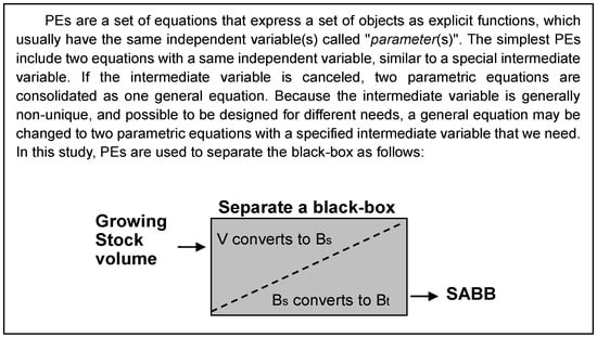
Figure 1.
A diagram of volume-SABB relationship analysis borrowing a simple concept from black-box system identification. The gray rectangle is assumed as a black-box. It includes two sub-modules (Bt and Bs) expressed by Parametric Equations (PEs).
2.2. Parametric Equations
In applications of functions and equations, a set of PEs is mainly utilized to solve problems in multidimensional space for convenience of mathematical treatment. Beyond this, the PEs may also express some physical or physiological quantity to clearly and more effectively describe the relationship between the parameter and its function. Here, the parameter (parameter variable) is mathematically specified as the independent variable in a set of PEs (see Figure 1). This special relationship is the key that we want to pay more attention to in our analysis. Hence, we introduce a parameter variable Bs (stem biomass, t ha−1) and make a pair of equations to separate the error source: Bt = aBsb and V = Bs/ρ. For general expression, we give the following PEs,
where Bt denotes SABB (t ha−1), a and b are parameters of the allometric function, and V is growing stock volume (m3 ha−1). ρ expresses average wood density for a regression parameter, as no assumption is made that wood density does not change with age, growing conditions, and species.
Bt = Bsb,
Bs = ρV,
Both Equations (1) and (2) are regression equations, in which all parameters (a, b, ρ) are determined by regression analysis. Equation (1) reflects tree physiological characteristics, which is expressed as the allometric relationship between stem biomass and SABB; Equation (2) indicates physical characteristics, which shows a linear relationship of stem biomass and volume with a slope coefficient ρ. The undetermined parameters a and b are solvable since field measurements of both stem biomass and SABB are available. While parameterizing the two equations, we can examine whether the parameters are reasonable and reliable, depending on our tree physiological and wood physical knowledge. Figure 2 illustrates an example of the parameterization. If all parameters (a, b, and ρ) are reasonable, there must be a “restricted zone” existing between the curves of the two equations (Figure 2B), assuming (1) a stem is lighter than the whole tree, and (2) ρ is equal to wood density and generally less than 1.0 (t m−3). This restricted zone can be defined as a zone where observed data should not lie unless there are errors or anomalies in the data. Any observed data lying in the restricted zone strongly suggests that there may be problems in field measurement or counting. After fixing these problems by setting up restrictions on regression parameters, the reliability of these two PEs will be improved and Equations (1) and (2) can then be rewritten as a conventional single equation by canceling Bs:
where Bt denotes SABB (t ha−1), V is volume density (m3 ha−1), and α and β are parameters. Thus, two models have been built, the PE model (Equations (1) and (2)) and the conventional model (Equation (3)). The parameters of the two models can be substituted by one another as α = aρb, β = b.
Bt = αVβ,
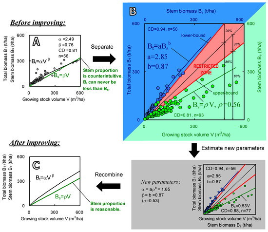
Figure 2.
An example (Eucalyptus and other fast-growing trees in China) of the regression for Equations (1) and (2). (A) is the plots and regression with general equation Bt = αVβ. The green line graphs equation Bs = ρV. (B) exhibits two regressions outside the restricted zone separately. The correlation scatters of SABB vs. stem biomass (blue and top left part) and stem biomass vs. stem volume (green and bottom right part). The top left parts illustrate the regression for Equation (1), and bottom right parts do this for Equation (2). A restricted zone is designed ranging from the lower-bound of Bt (shows a proportion as 80% stem and 20% other parts of the tree) to upper-bound of Bs (shows maximum wood density of 0.7). The samples of Bs vs. Bt are less than the ones of Bs vs. V, because some plots were not measured for roots. (C) shows the recombined equation using the slope ρ after data cleaning.
2.3. Parameter Improvement
To follow the above strategy and formulation, two points should be noted: (i) improving parameters by utilizing PEs is a “separate-to-recombine” process (see Figure 2). After the improvement, the power β in Equation (3) is same as the power b in Equation (1). This is because the curvature of Equation (3) is only affected by the allometric relationship of Bs and Bt, but not by volume (V). If directly regressing field data for the variables Bt and V in Equation (3), the power β will usually be impacted more or less by possible outliers of the volume (V). Outliers make wood density estimates (ρ) largely inconsistent, which changes the curvature (β) of Equation (3). In short, the α and β will change after carrying out separate-to-recombine processing that forces ρ to be unique for a specified species. (ii) Through the separate-to-recombine procedure, the impacts of uncertainty or mistake in volume measurement can be excluded from parameter β. This allows us to concentrate on improving the parameter α by examining ρ. The necessity of the improvement is also illustrated in Figure 2A, in which the direct regression curve goes so far as to cross the line of Bs = ρV at the end. It clearly proves a counterintuitive relationship that may appear by performing regression analysis directly: stem biomass is greater than SABB. Summarily, we first separate the equation into two PEs (Figure 2A). Secondly, carry out regressions respectively for the two equations (Figure 2B). Then combine the two equations back into one standard volume-SABB equation as was the original form (Figure 2C). During this procedure, it should be emphasized that the restricted zone may be variable depending on different species.
2.4. Data Description
We used two data sources: field measurements and forest inventory. The measurements were utilized for fitting and parameterizing volume-SABB equations. The inventory is a part of China’s NFI, which contains total volume and area of Eucalyptus forests across the country. This statistical volume information was employed to convert forest biomass from volume using the volume-SABB model. The field measurements used in this study are abundant and diversified on species. They consist of three large datasets based on over 10,840 records, which were collected from a large data compilation from European, USA, Chinese, and Japanese scientific literatures (by Usoltsev [47], 8033 records; Luo et al. [48], 1607 records, see supporting information (Table S2); Cannell [49], over 1200 records). Most of records include data items of growing stock volume (V), stem biomass (Bs), AGB (foliage, branch, and stem), and BGB (coarse and fine roots) per hectare. The destructive measurements were carried out for AGB. Roots were completely dug out or partly dug out for BGB estimations. The biomasses in the datasets were expressed in oven-dry weight and measured based on felled trees at each plot. Since data from Luo et al. [48] are the latest collection for China’s forests, we excluded all records of measurements in China from the Usoltsev’s dataset. Of the total 10,840 sample records assembled in the three datasets, applicable data (3649 records) processed correspond to 3335 records for stem biomass and SABB, and 3399 records for growing stock volume and stem biomass. For Luo et al. [48] and Usoltsev [47] the trees were basically grouped by species, while for Cannell [49] all trees were grouped by forest types (conifer, broadleaved, mixed, and tropical forest). All field data were compiled and up-scaled from tree and plot data to hectare-based values by data providers.
2.5. Coverage Area of Observations
The spatial locations of all field plots in the datasets are widely distributed geographically in 48 countries around the world (Figure 3). The measurements were carried out for over 317 tree species. The dataset includes different forest types at different latitudes and climatic conditions. These plots are dispersed over boreal temperate, subtropical, and tropical zones with forest ages from young stands of about 5 years to over mature forest of more than 400 years. Main types of woody plant stands are represented including those from natural and plantation forest origins, ranging from oak woodlands and coniferous plantations to tropical rainforests and mangrove swamps. The distribution of plots is uneven across continents and they are highly concentrated in some countries (Figure 3).
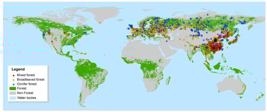
Figure 3.
Spatial distribution of all plots measured across the world [50,51].
2.6. Sampling Simulation
To test the numerical stability of model parameters, we made a pseudo population to simulate the true values of a large-scale forest. This population consists of 10,000 forest stands at the regional scale based on the output of a pseudorandom number generator. The true values of SABB amount (5.18 Mt) are counted by enumerating all pseudo stands in the population for model comparisons. Our experiment carried out random samplings, which simulate the establishing of a few sample plots (or the collecting of field data). We firstly generated the values of three variables (Area, V, and ρ) for each stand. ρ was generated in two conditions as constant and random value. Bs can be calculated. Then Bt can be generated. Based on this population of pseudo stands (10,000 stands), we selected four types of stand samples from the population. The sampling design consists of four types, such as 20 stands with ρ = 0.59, 100 stands with ρ = 0.59, 20 stands with random ρ, 100 stands with random ρ. Each sampling rule was performed 500 times. The model outputs were compared between before and after the improvement of parameters (α and β). The details of data structure, data plotting, and simulation conditions are described in the Supporting Information (Table S1 and Figure S1).
3. Results
3.1. Comparison of Two Relationships
We respectively analyzed three independent data sources published at different times (refer to Table 1). Our results report that the relationship between Bs and Bt has a better fitting performance than V and Bs (Figure 4). Most coefficients of determination for Bs vs. Bt are greater than 0.9. In the bottom right part of each scatter plot, Bs and V have a significant linear relationship with all coefficients of determination greater than 0.6, although a few samples are located in the restricted zones for some species and forest types (No. 8, 10, 15, 18, 25, 27, 29, 30). All regression curves (Bs-to-Bt) and lines (V-to-Bs) avoid falling in the “restricted zones.”

Table 1.
Parameters in Equations (1)–(3) for 30 tree species and forest types across the world.
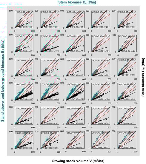
Figure 4.
The correlation scatters of 30 tree species and forest types across the world. The least squares regression was performed for fitting V-to-Bs equation. The nonlinear regressions were conducted for fitting relationships of Bt and Bs. The scatters show stem biomass vs. SABB (curves with cyan crosses in top left sections) and growing stock volume vs. biomass (straight-lines with black crosses in bottom right sections). The top left parts illustrate the regression for Equation (1), and bottom right parts do this for Equation (2). CD means coefficient of determination; n is the numbers of plots. Every scatter has two red lines that warn the lower limit for Equation (1) and the upper limit for Equation (2). Note that these red lines are set up tentatively for approximate estimates of the restricted zone that may change for different species and types. The number of each scatter corresponds to the number listed in Table 1. Three variables (volume, stem, and SABB) were measured for most plots. The samples of Bs vs. Bt are less than the ones of V vs. Bs, because some plots were not measured for roots or volumes. For the data details refer to the footnotes of Table 1.
The modeling parameters (a, b, and ρ) are listed in Table 1 for 30 species and forest types. The values of b are distributed in the vicinity of 0.9 and the values of α have a wide range from 1.88 (No. 25) to 4.5 (No. 6). As for the estimated ρ, which is the slope of the regressed straight-lines in Figure 4, all values are less than 0.7 (t m−3). Tropical trees have a relatively high wood density with values greater than 0.6 (t m−3). The “data cleaning” was carried out based on the range of wood basic densities (WBD), which were from the data in the Global Wood Density (GWD) database [52]. The WBDs of all species and forest types range from 0.3 to 0.8 (t m−3). All data points that fell into the restricted zone mean that the data make the ratio of stem biomass to SABB higher than 0.8 (t m−3). After taking off those irregular observations, the ρ and α were re-estimated and listed in Table 1 (in the 7th and 10th columns).
3.2. Model Test
After determining a, b and ρ, the parameter α in volume-SABB equation (Equation (3)) can be calculated as α = aρb before data cleaning. The standard deviations of ρ are lower than 5.5% for all non-tropical species, and less than 7.4% for tropical species (Table 1). The equation was tested under two cases (Table 2), (1) all stands have the same ρ and same ratio of stem to SABB, and also have no measurement errors either; (2) the ρ and ratio become dispersible with measurement errors. Corresponding to these cases, 500 sampling simulations demonstrated that the mathematical expectations (see μ values in the e column in Table 2) of model errors (absolute value of residuals) become lower than before after improving the parameters, whether by 20-plot-sampling or 100-plot-sampling. Table 2 demonstrates that improved parameters decreased residual errors by up to 50% than the original parameters did.
Table 2.
The comparison between the results before and after improving parameters (α and β) of volume-SABB equations. These equations are regressed based on the simulation data (refer to Supporting Information Table S1). Parameter (α and β) and residual distributions resulted from 500 simulations of setting field plot.
In addition, Figure 5 illustrates a comparison between distributions of the parameter (α and β) and residual (e), which denotes the difference between two estimations before and after improving the parameters based simulated data. The distributions of α, β, and e resulted from 500 simulations of setting stands. It is visible that improved α, β, and e generally have low standard deviations for both sampling designs (20-plot- and 100-plot-sampling). The convergence rates are faster on 100-plot-sampling than 20-plot-sampling for all tests of α, β, and e (Figure 5). This implies that the estimates are closer to the true value (5.18 Mt) by employing the 100-plot-sampling design than the 20-plot-sampling design.
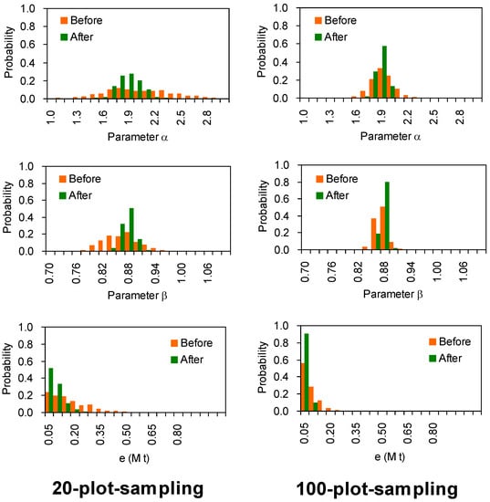
Figure 5.
Comparison between two estimations before and after improving the parameters based simulated pseudo data. Averaged parameters (α and β) and residual (e) distributions resulted from 500 simulations of setting field plot. The model estimates are calculated using Equation (3) with parameters before and after improvement. For the data details refer to the footnotes of Table 2.
3.3. Comparison Between Biomass Estimates
To understand the differences of SABB amounts affected by variant wood densities, we estimated the biomass of China’s Eucalyptus forests, which are scattered in 10 provinces over a large area (total 4455.2 K ha) [53]. The allometric equation and parameters are shown in Figure 2 (before improving: Bt = 2.49V0.76; after improving: Bt = 1.72V0.87). These two equations result in large gaps. If using the three wood densities, the SABB amount increases to 173 (+3%) Mt from 1.68 Mt after improving parameters (α and β). This implies that different estimates of wood density could produce considerable gaps.
4. Discussion
4.1. Model Test
There are two common ways to test a model and evaluate if it is better than others. A widely used method is the comparison between prediction and independent observation [54]. Yet we do not have other field data independent of the measurements used in this study. Another way is statistical hypothesis testing, which rejects or fails to reject (does not equal accept) the null hypothesis [55]. However, the significance level or p-value provided by a parameter test cannot prove that a model result is closer to the true value than other models. A previous study [21] indicated that model tests are always difficult for the immeasurable forest population on large-scales. Given this consideration, we made a pseudo population to realize the “true values” of a large-scale forest. In our experiment, we focus on the sample population. This approach is a low-cost way to acquire the “true value” of a population and use the “true value” to test if the model has generality for application.
The pseudo population provided two true values (5.19 and 5.18 Mt) of total SABB by specifying two kinds of wood densities (a constant, and random value fitting the normal distribution). Our results suggest that the recombined equation is better than the original equation in model performance as total SABB is closer to the true value after improving parameters. The results of parameter diagnosis revealed two major points: (1) if all stands have the same features (ρ and the ratio of stem biomass to SABB) and have no measurement errors either, it makes no difference (Table 2) whether the equation is improved or not via the separate-to-recombine processing. (2) As long as the plot features become dispersible in realistic forests, and the errors occur in practical measurements [56], the equation improvement results in different parameters. It implies that PEs with a parameter ρ is advantageous for improving the accuracy of biomass prediction. This supports previous analyses of using wood density as a parameter in biomass equations [25,40,57,58].
Furthermore, two trial sampling designs were carried out for obtaining different samples (20 and 100 stands) in the pseudo population. Through comparing parameters and the estimates of SABB amount, our results imply that more measurements will have better representativeness for the population. This evidence on the significant effects of sample size on biomass estimates is consistent with previous studies [13,59]. The results based on the sampling designs are also in accordance with reported analyses [8,14,21,22,39,42,43,55]. In addition to the pseudodata test, a practical estimation was carried out for China’s Eucalyptus on the large scale. Comparing the equation before improvement, the gap is approximately 3% between SABB amount before and after parameter improvement. Overall our experiment demonstrated a positive effect on model accuracy based on the processing of separating regressions.
4.2. Wood Density Estimation
Testing the equations of V-to-Bs, the standard deviations of ρ are relatively low. All regression lines are below the restricted zone, because the slopes (ρ) express wood density as the value of mathematical expectation in a normal distribution. This means that some outliers do not have a great impact on the regression. The reason for produced outliers is complicated [60]. A number of studies have reported that wood density may vary over broad geographic areas [29,56,61,62] and also between individual trees and different organs [63,64]. Flores and Coomes [59] investigated wood densities for 8412 species from the Global Wood Density (GWD) database [52] and indicated that the mean relative error ranges from ±10% to ±31% for different countries. These analyses at tree-level are consistent with our results at plot-level.
According to the field measurements, graphic analysis illustrated different ratios of stem biomass to volume for the same species in (Figure 2B and Figure 4), especially for young stands with low volume. To address this difference, our study utilized linear regression. Notwithstanding the variance, the mathematical expectation describes the weighted mean of all plot samples (combined) under various geographical and environmental conditions. We suggest that the abnormal values of a few ratios may not be a significant issue in this study. Nonetheless, we re-estimated the parameters of ρ and α by excluding all data points located in the restricted zone. The difference between α before and after data cleaning ranges from −3.7% to 3.9% for most of the species and types. This implies that abnormal values of most ratios do not significantly affect the models. However, type #9 has a difference of −11.7% after data cleaning, because several data points (whose ratio of stem biomass to SABB is less than 0.3 t m−3) were excluded. It implies that the data and ratio need to be carefully confirmed for “other conifer trees” in the application.
4.3. Uncertainties
The results indicate that conventional volume-SABB equations may introduce more errors than PEs in a biomass estimation of forest ecosystems. This probably is a problem caused by the equation structure, for which some studies [14,22,65] have discussed regarding the effect on the estimates. After separating the estimation of stem (Equation (2)) and SABB (Equation (1)), the effect of equation structure is reduced for the latter. However, the former is highly dependent on wood density [13]. We noticed that some sample points (black cross marks, Figure 4) are over the 45° line. These ratios of stem biomass to volume (i.e., wood density) become higher than 1.0 t m−3, which becomes a concern. We tend to think that the measurement issue may be found in the measurements of volume, rather than stem biomass. Most plot points above the 45° lines represent lower volume than other points below the lines (Figure 4). It should not be like this for most species. For example, the species #11 (Populus and Betula) has a few sample points (close to lower left, Figure 4) located in the restricted zone, but fast-growing species generally have low densities in their juvenile wood, especially for the first one or two decades [66,67]. Denslow [68] also reported that wood density is low for pioneer trees in succession. These seem to be contradictory. It implies that the volume measurement issue may be, in some cases, a problem of parameterization for conventional volume-SABB equations. We suggest checking the ratio of stem biomass to volume when scaling the measurements from tree-level to plot-level.
Technically, in terms of destructive measurement, it could be easier to destructively measure each organ biomass (e.g., foliage, branch, stem, and coarse and fine root) of a few trees accurately than to measure and evaluate the growing stock volume (m−3 ha−1) for the unit area. There are many error sources in real volume estimation. The errors may be introduced from measuring the volume of single trees [69,70]. Additionally, the volume at plot-level calculation may cause statistical errors due to the heterogeneity of each stem form and diameter class [71]. Moreover, the definition of stem could also influence the parameterization [14,22]. Hence, volume measurements might principally affect the ratio of stem biomass to volume. Our analysis revealed that the measurements of stem and other organ biomass cause uncertainty (Equation (1)) less than volume does (Equation (2)). For instance, graphical analyses did not show the indication of heterogeneity in the relationship between stem biomass and SABB for any species or forest types (see Figure 4). Figure 4 illustrates that the coefficients of determination (CD) range from 0.81 to 0.99 for Equation (1) (the top half of each subplot), which is better than the range of 0.62–0.96 for Equation (2) (the bottom half of each subplot). The observed stem biomass suggests a relatively large and stable portion of SABB regardless of a single tree or plots based on the dataset [47]. We found that the percentage of stem in SABB is averaged as 67.96% (SD = 7.83%, n = 1502). This percentage is consistent with the global patterns in forest biomass reported by Reich et al. [72]. In contrast, ratios of stem biomass to volume were spread over a wide range. The data marks (Figure 2B and Figure 4) invaded the “restricted zone” more frequently in the bottom left rather than the top right of the figure. All these imply that measurements are more reliable for stem than volume.
In addition to the volume issue, the small sample size has been considered to limit the estimate accuracy [23]. In our datasets, four species or forest types have less than 20 plot samples for the relationship between stem biomass and SABB; six species or forest types have less than 20 plot samples for the ratio of stem biomass to volume. The sample size of individual tree has the same issue. Jenkins et al. [73] reported that nearly half of the studies had sample sizes of 20 trees or less for 2642 equations in the United States. This implies a superior difficulty in obtaining field measurements of tree volume and organ biomasses over a wide geographic area. The limited size of the dataset affects models in terms of their application over large spatial domains [8]. For such species that have few and rare samples, we strongly suggest using PEs as an alternative option to compare the relationship of volume-to-SABB. The regressions of PE allow WBD or the wood specific gravity to act as an inspector to check the rationality of the data.
5. Conclusions
The hectare-based volume-SABB equation is a valuable tool for depicting the relationship between stem volume and SABB (stand above- and below-ground biomass) at stand-level. It is a realistic way to estimate forest biomass using hectare-based volume-SABB equations for many countries, whose NFI reports currently do not contain detailed information of DBH and tree height. The PE method is a convenient tool for reducing uncertainty in the relationship of forest volume and SABB based on limited field plots. The graphical representation of PEs proposes a concept of “restricted zone,” which helps to diagnose the volume-SABB relationship in regression analyses of field data at stand-level. By obeying the limits of a “restricted zone,” the knowledge of wood densities can act as an inspector for checking field data. The presented analyses of formulating volume-SABB equations suggest an applicable method for restricting the error in field data processing, and achieving a better understanding of the uncertainty in building those equations at stand-level. Diagnosed volume-SABB equations will hopefully be able to play a significant part in estimations of forest carbon sequestration and carbon balance at any large scale.
Supplementary Materials
The following are available online at https://www.mdpi.com/1999-4907/10/8/658/s1, Figure S1. Simulated stands as a forest population for the model testing experiment. The stand number corresponds to the number in Table S1; Table S1. The simulated data set, based on two assumptions with even (0.59, t m−3) and randomly distributed for constructing a pseudo stand population in a large region (10,000 stands, assuming Eucalyptus); Table S2. Measurements of volume and biomass in China. The data include both measured volume and biomasses of each tree organs for 261 species at 1607 field plots over the country.
Author Contributions
X.Z. and C.L. conceived this study, performed mathematical analysis, and wrote the manuscript; C.L., X.Z., X.L., H.H., C.P., and X.W. discussed algorithm improvement, paper structure, and conclusions; C.L. and C.Z. conducted the data collection, data analysis, and manuscript preparation. All authors read and approved the final manuscript.
Funding
This work was supported by The National Key Research and Development Program of China (2017YFA0604401, 2016YFC0501101), Open Fund of State Key Laboratory of Remote Sensing Science (OFSLRSS201704) and Meteorology Scientific Research Fund in the Public Welfare of China (GYHY201506010).
Acknowledgments
We thank Vladimir A. Usoltsev for providing all data and documents in the publication Biomass and Primary Production of Eurasian Forests. We are also grateful to the two anonymous reviewers for their insightful comments and valuable suggestions. We appreciate the corresponding editors for their very helpful suggestions.
Conflicts of Interest
The authors declare no conflict of interest.
References
- Mitchard, E.T.A. The tropical forest carbon cycle and climate change. Nature 2018, 559, 527–534. [Google Scholar] [CrossRef] [PubMed]
- Rodriguez-Veiga, P.; Quegan, S.; Carreiras, J.; Persson, H.J.; Fransson, J.E.S.; Hoscilo, A.; Ziolkowski, D.; Sterenczak, K.; Lohberger, S.; Stangel, M.; et al. Forest biomass retrieval approaches from earth observation in different biomes. Int. J. Appl. Earth Obs. Geoinf. 2019, 77, 53–68. [Google Scholar] [CrossRef]
- Lu, D. The potential and challenge of remote sensing-based biomass estimation. Int. J. Remote Sens. 2006, 27, 1297–1328. [Google Scholar] [CrossRef]
- Seidel, D.; Fleck, S.; Leuschner, C.; Hammett, T. Review of ground-based methods to measure the distribution of biomass in forest canopies. Ann. For. Sci. 2011, 68, 225–244. [Google Scholar] [CrossRef]
- Dobbertin, M.; Neumann, M.; Schroeck, H.-W. Chapter 10—Tree Growth Measurements in Long-Term Forest Monitoring in Europe. In Developments in Environmental Science; Elsevier: Amsterdam, The Netherlands, 2013; pp. 183–204. [Google Scholar]
- Liang, X.; Kukko, A.; Hyyppa, J.; Lehtomaki, M.; Pyorala, J.; Yu, X.; Kaartinen, H.; Jaakkola, A.; Wang, Y. In-situ measurements from mobile platforms: An emerging approach to address the old challenges associated with forest inventories. ISPRS J. Photogramm. Remote Sens. 2018, 143, 97–107. [Google Scholar] [CrossRef]
- Mayaka, T.B.; Eba, R.; Momo, S.T. Construction of multi species allometric equations: Is there a statistical palliative for destructive tree sampling? J. Trop. For. Sci. 2017, 29, 282–296. [Google Scholar]
- Weiskittel, A.R.; MacFarlane, D.W.; Radtke, P.J.; Affleck, D.L.R.; Temesgen, H.; Woodall, C.W.; Westfall, J.A.; Coulston, J.W. A Call to Improve Methods for Estimating Tree Biomass for Regional and National Assessments. J. For. 2015, 113, 414–424. [Google Scholar] [CrossRef]
- Addo-Danso, S.D.; Prescott, C.E.; Smith, A.R. Methods for estimating root biomass and production in forest and woodland ecosystem carbon studies: A review. For. Ecol. Manag. 2016, 359, 332–351. [Google Scholar] [CrossRef]
- Paul, K.I.; Larmour, J.; Specht, A.; Zerihun, A.; Ritson, P.; Roxburgh, S.H.; Sochacki, S.; Lewis, T.; Barton, C.V.M.; England, J.R.; et al. Testing the generality of below-ground biomass allometry across plant functional types. For. Ecol. Manag. 2019, 432, 102–114. [Google Scholar] [CrossRef]
- Somogyi, Z.; Cienciala, E.; Mäkipää, R.; Muukkonen, P.; Lehtonen, A.; Weiss, P. Indirect methods of large-scale forest biomass estimation. Eur. J. For. Res. 2007, 126, 197–207. [Google Scholar] [CrossRef]
- Brown, S.L.; Lugo, A. Biomass of Tropical Forests: A New Estimate Based on Forest Volumes Author (s): Sandra Brown and Ariel E. Lugo Published by: American Association for the Advancement of Science Stable. Science 1984, 223, 1290–1293. [Google Scholar] [CrossRef] [PubMed]
- Ver Planck, N.R.; MacFarlane, D.W. A vertically integrated whole-tree biomass model. Trees Struct. Funct. 2015, 29, 449–460. [Google Scholar] [CrossRef]
- Neumann, M.; Moreno, A.; Mues, V.; Härkönen, S.; Mura, M.; Bouriaud, O.; Lang, M.; Achten, W.M.J.; Thivolle-Cazat, A.; Bronisz, K.; et al. Comparison of carbon estimation methods for European forests. For. Ecol. Manag. 2016, 361, 397–420. [Google Scholar] [CrossRef]
- Jucker, T.; Caspersen, J.; Chave, J.; Antin, C.; Barbier, N.; Bongers, F.; Dalponte, M.; van Ewijk, K.Y.; Forrester, D.I.; Haeni, M.; et al. Allometric equations for integrating remote sensing imagery into forest monitoring programmes. Glob. Chang. Biol. 2017, 23, 177–190. [Google Scholar] [CrossRef] [PubMed]
- Di Cosmo, L.; Gasparrini, P.; Tabacchi, G. A national-scale, stand-level model to predict total above-ground tree biomass from growing stock volume. For. Ecol. Manag. 2016, 361, 269–276. [Google Scholar] [CrossRef]
- Guo, Z.; Fang, J.; Pan, Y.; Birdsey, R. Inventory-based estimates of forest biomass carbon stocks in China: A comparison of three methods. For. Ecol. Manag. 2010, 259, 1225–1231. [Google Scholar] [CrossRef]
- Jenkins, J.C.; Chojnacky, D.C.; Heath, L.S.; Birdsey, R.A. National-Scale Biomass Estimators for United States Tree Species. For. Sci. 2003, 49, 12–35. [Google Scholar]
- Zianis, D.; Seura, S. Biomass and stem volume equations for tree species in Europe. Silva Fenn. Monogr. 2005, 4, 1–63. [Google Scholar]
- Muukkonen, P.; Heiskanen, J. Biomass estimation over a large area based on standwise forest inventory data and ASTER and MODIS satellite data: A possibility to verify carbon inventories. Remote Sens. Environ. 2007, 107, 617–624. [Google Scholar] [CrossRef]
- Henry, M.; Picard, N.; Trotta, C.; Manlay, R.J.; Valentini, R.; Bernoux, M.; Saint-André, L. Estimating tree biomass of sub-Saharan African forests: A review of available allometric equations. Silva Fenn. 2011, 45, 477–569. [Google Scholar] [CrossRef]
- Boudewyn, P.; Song, X.; Magnussen, S.; Gillis, M.D. Model-Based, Volume-to-Biomass Conversion for Forested and Vegetated Land in Canada; Natural Resources Canada Canadian Forest Service Pacific Forestry Centre Natural: Victoria, BC, Canada, 2007; p. 124.
- Segura, M.; Kanninen, M. Allometric models for tree volume and total aboveground biomass in a tropical humid forest in Costa Rica. Biotropica 2005, 37, 2–8. [Google Scholar] [CrossRef]
- Smith, J.E.; Heath, L.S.; Jenkins, J.C. Forest Volume-to-Biomass Models and Estimates of Mass for Live and Standing Dead Trees of US Forests; Department of Agriculture, Forest Service: Newtown Square, PA, USA, 2003; p. 57.
- Zhou, X.; Lei, X.; Peng, C.; Wang, W.; Zhou, C.; Liu, C.; Liu, Z. Correcting the overestimate of forest biomass carbon on the national scale. Methods Ecol. Evol. 2016, 7, 447–455. [Google Scholar] [CrossRef]
- Nelson, R.; Margolis, H.; Montesano, P.; Sun, G.; Cook, B.; Corp, L.; Andersen, H.E.; deJong, B.; Pellat, F.P.; Fickel, T.; et al. Lidar-based estimates of aboveground biomass in the continental US and Mexico using ground, airborne, and satellite observations. Remote Sens. Environ. 2017, 188, 127–140. [Google Scholar] [CrossRef]
- Chen, Q.; Vaglio Laurin, G.; Valentini, R. Uncertainty of remotely sensed aboveground biomass over an African tropical forest: Propagating errors from trees to plots to pixels. Remote Sens. Environ. 2015, 160, 134–143. [Google Scholar] [CrossRef]
- Lu, D.; Chen, Q.; Wang, G.; Liu, L.; Li, G.; Moran, E. A survey of remote sensing-based aboveground biomass estimation methods in forest ecosystems. Int. J. Digit. Earth 2016, 9, 63–105. [Google Scholar] [CrossRef]
- Henry, M.; Besnard, A.; Asante, W.A.; Eshun, J.; Adu-Bredu, S.; Valentini, R.; Bernoux, M.; Saint-André, L. Wood density, phytomass variations within and among trees, and allometric equations in a tropical rainforest of Africa. For. Ecol. Manag. 2010, 260, 1375–1388. [Google Scholar] [CrossRef]
- Mather, A.S. Assessing the world’s forests. Glob. Environ. Chang. 2005, 15, 267–280. [Google Scholar] [CrossRef]
- Lei, X.; Tang, M.; Lu, Y.; Hong, L.; Tian, D. Forest inventory in China: Status and challenges. Int. For. Rev. 2009, 11, 52–63. [Google Scholar] [CrossRef]
- FAO. Global Forest Resources Assessment 2010; Food and Agriculture Organization of the United Nations: Rome, Italy, 2010. [Google Scholar]
- Fang, J.; Chen, A.; Peng, C.; Zhao, S.; Chi, L. Changes in forest biomass carbon storage in China between 1949 and 1998. Science 2001, 292, 2320–2322. [Google Scholar] [CrossRef]
- Pan, Y.; Luo, T.; Birdseyi, R.; Hom, J.; Melill, J. New estimates of carbon storage and sequestration in china’s forests: Effects of age-class and method on inventory-based carbon estimation. Clim. Chang. 2004, 67, 211–236. [Google Scholar] [CrossRef]
- Xu, X.; Li, K. Biomass carbon sequestration by planted forests in China. Chin. Geogr. Sci. 2010, 20, 289–297. [Google Scholar] [CrossRef]
- Zhang, C.; Ju, W.; Chen, J.M.; Zan, M.; Li, D.; Zhou, Y.; Wang, X. China’s forest biomass carbon sink based on seven inventories from 1973 to 2008. Clim. Chang. 2013, 118, 933–948. [Google Scholar] [CrossRef]
- Du, L.; Zhou, T.; Zou, Z.; Zhao, X.; Huang, K.; Wu, H. Mapping forest biomass using remote sensing and national forest inventory in China. Forests 2014, 5, 1267–1283. [Google Scholar] [CrossRef]
- Hu, H.; Wang, S.; Guo, Z.; Xu, B.; Fang, J. The stage-classified matrix models project a significant increase in biomass carbon stocks in China’s forests between 2005 and 2050. Sci. Rep. 2015, 5, 11203. [Google Scholar] [CrossRef]
- Parresol, B.R. Assessing tree and stand biomass: A review with examples and critical comparisons. For. Sci. 1999, 45, 573–593. [Google Scholar]
- Chave, J.; Muller-Landau, H.C.; Baker, T.R.; Easdale, T.A.; Steege, H.T.; Webb, C.O. Regional and phylogenetic variation of wood density across 2456 Neotropical Tree Species. Ecol. Appl. 2006, 16, 2356–2367. [Google Scholar] [CrossRef]
- Ni, J. Carbon storage in Chinese terrestrial ecosystems: Approaching a more accurate estimate. Clim. Chang. 2013, 119, 905–917. [Google Scholar] [CrossRef]
- Sileshi, G.W. A critical review of forest biomass estimation models, common mistakes and corrective measures. For. Ecol. Manag. 2014, 329, 237–254. [Google Scholar] [CrossRef]
- Temesgen, H.; Affleck, D.; Poudel, K.; Gray, A.; Sessions, J. A review of the challenges and opportunities in estimating above ground forest biomass using tree-level models. Scand. J. For. Res. 2015, 30, 326–335. [Google Scholar] [CrossRef]
- Lindner, M.; Fitzgerald, J.B.; Zimmermann, N.E.; Reyer, C.; Delzon, S.; Van Der Maaten, E.; Schelhaas, M.J.; Lasch, P.; Eggers, J.; Van Der Maaten-Theunissen, M.; et al. Climate change and European forests: What do we know, what are the uncertainties, and what are the implications for forest management? J. Environ. Manag. 2014, 146, 69–83. [Google Scholar] [CrossRef]
- Wang, J.R.; Zhong, A.L.; Kimmins, J.P. Biomass estimation errors associated with the use of published regression equations of paper birch and trembling aspen. North. J. Appl. For. 2002, 19, 128–136. [Google Scholar]
- Soderstrom, T.; Stoica, P. System Identification; Prentice Hall: New York, NY, USA, 1989. [Google Scholar]
- Usoltsev, V.A. Forest Biomass and Primary Production Database for Eurasia, 2nd ed.; CD-ve.; Ural State Forest Engineering University: Yekaterinburg, Russia, 2013. [Google Scholar]
- Luo, Y.; Wang, X.; Zhang, X.; Lu, F. Biomass and Its Allocation of Forest Ecosystems in China; Chinese Forestry Publishing House Press: Beijing, China, 2013. [Google Scholar]
- Cannell, M.G.R. World Forest Biomass and Primary Production Data; Academic Press: London, UK, 1982. [Google Scholar]
- Gong, P.; Wang, J.; Yu, L.; Zhao, Y.; Zhao, Y.; Liang, L.; Niu, Z.; Huang, X.; Fu, H.; Liu, S.; et al. Finer resolution observation and monitoring of global land cover: First mapping results with Landsat TM and ETM+ data. Int. J. Remote Sens. 2013, 34, 2607–2654. [Google Scholar] [CrossRef]
- Yu, L.; Wang, J.; Li, X.; Li, C.; Zhao, Y.; Gong, P. A multi-resolution global land cover dataset through multisource data aggregation. Sci. China Earth Sci. 2014, 57, 2317–2329. [Google Scholar] [CrossRef]
- Zanne, A.; Lopez-Gonzalez, G.; Coomes, D.; Ilic, J.; Jansen, S.; Lewis, S.; Miller, R.; Swenson, N.; Wiemann, M.; Chave, J. Global Wood Density Database. 2009. Available online: http://datadryad.org/handle/10255/dryad.235 (accessed on 25 September 2016).
- CMF (Chinese Ministry of Forestry). Forest Resource Report of China for Periods 2008–2012; Department of Forest Resource and Management, Chinese Ministry of Forestry: Beijing, China, 2013.
- Picard, N.; Boyemba Bosela, F.; Rossi, V. Reducing the error in biomass estimates strongly depends on model selection. Ann. For. Sci. 2015, 72, 811–823. [Google Scholar] [CrossRef]
- Harrell, F.E., Jr. Regression Modeling Strategies: With Applications to Linear Models, Logistic and Ordinal Regression, and Survival Analysis, 2nd ed.; Springer: Heidelberg, Germany, 2015; Volume 64, ISBN 9783319194240. [Google Scholar]
- Chave, J.; Condit, R.; Lao, S.; Caspersen, J.P.; Foster, R.B.; Hubbell, S.P. Spatial and temporal variation of biomass in a tropical forest: Results from a large census plot in Panama. J. Ecol. 2003, 91, 240–252. [Google Scholar] [CrossRef]
- Domke, G.M.; Woodall, C.W.; Smith, J.E.; Westfall, J.A.; McRoberts, R.E. Consequences of alternative tree-level biomass estimation procedures on US forest carbon stock estimates. For. Ecol. Manag. 2012, 270, 108–116. [Google Scholar] [CrossRef]
- Chave, J.; Réjou-Méchain, M.; Búrquez, A.; Chidumayo, E.; Colgan, M.S.; Delitti, W.B.C.; Duque, A.; Eid, T.; Fearnside, P.M.; Goodman, R.C.; et al. Improved allometric models to estimate the aboveground biomass of tropical trees. Glob. Chang. Biol. 2014, 20, 3177–3190. [Google Scholar] [CrossRef]
- Flores, O.; Coomes, D.A. Estimating the wood density of species for carbon stock assessments. Methods Ecol. Evol. 2011, 2, 214–220. [Google Scholar] [CrossRef]
- Crowther, T.W.; Glick, H.B.; Covey, K.R.; Bettigole, C.; Maynard, D.S.; Thomas, S.M.; Smith, J.R.; Hintler, G.; Duguid, M.C.; Amatulli, G.; et al. Mapping tree density at a global scale. Nature 2015, 525, 201–205. [Google Scholar] [CrossRef]
- Chave, J.; Coomes, D.; Jansen, S.; Lewis, S.L.; Swenson, N.G.; Zanne, A.E. Towards a worldwide wood economics spectrum. Ecol. Lett. 2009, 12, 351–366. [Google Scholar] [CrossRef]
- Chave, J.; Condit, R.; Aguilar, S.; Hernandez, A.; Lao, S.; Perez, R. Error propagation and sealing for tropical forest biomass estimates. Philos. Trans. R. Soc. B Biol. Sci. 2004, 359, 409–420. [Google Scholar] [CrossRef]
- Baker, T.R.; Phillips, O.L.; Malhi, Y.; Almeida, S.; Arroyo, L.; Di Fiore, A.; Erwin, T.; Higuchi, N.; Killeen, T.J.; Laurance, S.G.; et al. Increasing biomass in Amazonian forest plots. Philos. Trans. R. Soc. B Biol. Sci. 2004, 359, 353–365. [Google Scholar] [CrossRef]
- Visser, M.D.; Bruijning, M.; Wright, S.J.; Muller-Landau, H.C.; Jongejans, E.; Comita, L.S.; de Kroon, H. Functional traits as predictors of vital rates across the life cycle of tropical trees. Funct. Ecol. 2016, 30, 168–180. [Google Scholar] [CrossRef]
- Woodall, C.W.; Heath, L.S.; Domke, G.M.; Nichols, M.C. Methods and Equations for Estimating Aboveground Volume, Biomass, and Carbon for Trees in the US Forest Inventory, 2010; Department of Agriculture, Forest Service: Newtown Square, PA, USA, 2011; p. 34.
- Kojima, M.; Yamamoto, H.; Yoshida, M.; Ojio, Y.; Okumura, K. Maturation property of fast-growing hardwood plantation species: A view of fiber length. For. Ecol. Manag. 2009, 257, 15–22. [Google Scholar] [CrossRef]
- Pretzsch, H.; Biber, P.; Schütze, G.; Kemmerer, J.; Uhl, E. Wood density reduced while wood volume growth accelerated in Central European forests since 1870. For. Ecol. Manag. 2018, 429, 589–616. [Google Scholar] [CrossRef]
- Denslow, J.S. Gap partitioning among tropical rainforest trees. Biotropica 1980, 12, 47–55. [Google Scholar] [CrossRef]
- Westfall, J.A.; Patterson, P.L. Measurement variability error for estimates of volume change. Can. J. For. Res. 2008, 37, 2201–2210. [Google Scholar] [CrossRef]
- Berger, A.; Gschwantner, T.; McRoberts, R.E.; Schadauer, K. Effects of measurement errors on individual tree stem volume estimates for the Austrian national forest inventory. For. Sci. 2014, 60, 14–24. [Google Scholar] [CrossRef]
- McRoberts, R.E.; Westfall, J.A. The effects of uncertainty in individual tree volume model predictions on the uncertainty of large area volume estimates the method. For. Sci. 2014, 60, 34–42. [Google Scholar]
- Reich, P.B.; Luo, Y.; Bradford, J.B.; Poorter, H.; Perry, C.H.; Oleksyn, J. Temperature drives global patterns in forest biomass distribution in leaves, stems, and roots. Proc. Natl. Acad. Sci. USA 2014, 111, 13721–13726. [Google Scholar] [CrossRef]
- Jenkins, J.C.; Chojnacky, D.C.; Heath, L.S.; Birdsey, R.A. Comprehensive Database of Diameter-Based Biomass Regressions for North American Tree Species; Department of Agriculture, Forest Service: Newtown Square, PA, USA, 2004; p. 45.


© 2019 by the authors. Licensee MDPI, Basel, Switzerland. This article is an open access article distributed under the terms and conditions of the Creative Commons Attribution (CC BY) license (http://creativecommons.org/licenses/by/4.0/).