Article

Modeling Dynamics of Structural Components of Forest Stands Based on Trivariate Stochastic Differential Equation

Agriculture Academy, Vytautas Magnus University, Kaunas 44248, Lithuania
Forests 2019, 10(6), 506; https://doi.org/10.3390/f10060506
Submission received: 26 April 2019 / Revised: 11 June 2019 / Accepted: 12 June 2019 / Published: 14 June 2019
(This article belongs to the Special Issue Modeling of Forest Structure and Dynamics)

Abstract

:
Research Highlights: Today’s approaches to modeling of forest stands are in most cases based on that the regression models and they are constructed as static sub-models describing individual stands variables. The disadvantages of this method; it is laborious because too many different equations need to be assessed and empirical choices of candidate equations make the results subjective; it does not relate to the stand variables dynamics against the age dimension (time); and does not consider the underlying covariance structure driving changes in the stand variables. In this study, the dynamical model defined by a fixed-and mixed effect parameters trivariate stochastic differential equation (SDE) is introduced and described how such a model can be used to model quadratic mean diameter, mean height, number of trees per hectare, self-thinning line, stand basal area, stand volume per hectare and much more. Background and Objectives: New developed marginal and conditional trivariate probability density functions, combining information generated from an age-dependent variance-covariance matrix of quadratic mean diameter, mean height and number of trees per hectare, improve stand growth prediction, and forecast (in forecast the future is completely unavailable and must only be estimated from historical patterns) accuracies. Materials and Methods: Fixed-and mixed effect parameters SDE models were harmonized to predict and forecast the dynamics of quadratic mean diameter, mean height, number of trees per hectare, basal area, stand volume per hectare, and their current and mean increments. The results and experience from applying the SDE concepts and techniques in an extensive whole stand growth and yield analysis are described using a Scots pine (Pinus sylvestris L.) experimental dataset in Lithuania. Results: The mixed effects scenario SDE model showed high accuracy, the percentage root mean square error values for quadratic mean diameter, mean height, number of trees per hectare, stand basal area and stand volume per hectare predictions (forecasts) were 3.37% (10.44%), 1.82% (2.07%), 1.76% (2.93%), 6.65% (10.41%) and 6.50% (8.93%), respectively. In the same way, the quadratic mean diameter, mean height, number of trees per hectare, stand basal area and stand volume per hectare prediction (forecast) relationships had high values of the coefficient of determination, R2, 0.998 (0.987), 0.997 (0.992), 0.997 (0.988), 0.968 (0.984) and 0.966 (0.980), respectively. Conclusions: The approach presented in this paper can be used for developing a new generation stand growth and yield models.

1. Introduction

In the forestry literature, two philosophically different streams of research have been used; statistical inference and mechanistic modeling mechanisms describe the relationships between whole-stand (thereafter-stand) variables [1,2,3]. First attempts to model stand growth and yield were done in Germany by Schwappach [4], and in Austria by Guttenberg [5]. At that time, graphical smoothing of empirical data was used to create relationships between stand-level dependent and response variables. Mathematical modeling of the stand yield and growth start in the middle of the 20th century by Assmann and Franz [6]. Stand density (number of trees per hectare), mean or max stand height, and quadratic diameter at breast height are fundamental stand variables when developing mathematical models for predicting and forecasting forest stand growth and yield. Quadratic mean diameter is the measure of the average tree diameter and stems from the exact relationship B = k × N × (Dq)2 (B is the basal area and k is a constant that depends on the measurement units used) [7]. The quadratic mean diameter assumes greater value than the arithmetic mean depending on the variance, W2, of the diameter, D (by the relationship (Dq)2 = D2 + W2). The quadratic mean diameter is essential for estimating product yields. Stand density denotes a quantitative measurement of the stand and evaluates the degree of stem crowding within a particular forest area. The interaction between stand density, mean height, quadratic mean diameter and volume for even-aged stands are graphically represented by stand density diagrams [8,9,10]. Stand density diagrams are average whole stand models those facilitate the stand density silvicultural management. The construction of the stand density diagrams was traditionally performed using regression techniques to fit the non-linear allometric or algebraic difference equations for the quadratic mean diameter, volume and number of trees per hectare [10,11]. The algebraic difference approach represents a four-variable prediction system that is suitable for modeling pooled cross-sectional and longitudinal data, remeasured at least once [12]. The state-space models ignore correlations between tree size components and stand density [11]. The relationship between mean tree size and stand density have received considerable attention by forest researchers and have many applications in stand growth and yield modeling [1].
The philosophy of the mean stand volume estimation is based on stand density, mean stand height, and quadratic mean stand diameter. Classical mathematical modeling of relationships between mean tree size and stand density have been framed in a linear form as ln(N) + β ln(S) = constant that varies with species and site (Reineke’s rule [13]) and nonlinear form as Dq = (β1Hβ2N + β3Hβ4), where N is the number of trees per hectare and S is some measure of stem size (mean stand height, H, quadratic mean diameter, Dq, or volume, V) (see [3]; and references therein). Traditionally, the linear regression relationship has been used to relate the number of trees per hectare and quadratic mean diameter [13]. The Reineke’s rule was initially used to establish the −3/2 power (Reineke’s β≈ −1.605 and varies little with species, age or site quality) law of self-thinning [14,15,16,17] and the universality of this exponent was documented by several researchers [18,19]. Reineke’s Rule curve is referred to as the ‘reference curve’ [13,15], which graphically represents the potential profile of the density and diameter relationships of a particular species across sites.
The natural mortality process is not a continuous one, and it can be mimicked by using the Markov type diffusion processes. The main assumptions are that the current state of a stand and random forces completely determines its future evolution; independently of the history of past silvicultural treatments. The linear regression relationships presented in previous studies [3,13] have provided information on the number of trees per hectare that can be predicted at a given quadratic mean diameter, however, they do not relate to the stand density dynamic against the age dimension (time), and do not consider the underlying covariance structure driving changes in the number of trees per hectare, mean height, and quadratic mean diameter.
Historically, pure and even aged stand growth models that estimate structure changes over time were related to diameter distribution functions [20]. In this study, we attempted to link different types of whole stand models over a large geographic area by developing a trivariate mixed effect parameters stochastic differential equation (SDE) framework for an integrated system in which models of different resolutions are related in a unified mathematical structure. The newly developed probability density function can therefore be used for different models of stand attributes such as quadratic mean diameter, mean height, number of trees per hectare, stand basal area, stand volume per hectare and much more.
In the few last decades, the modeling of stochastic phenomenon in all areas of applied sciences has incorporated fluctuations in the model parameters, state variables, and measurement errors that are omitted in deterministic models [21,22]. The first SDEs models were introduced to forestry by Suzuki (1971) [23] and Sloboda (1977) [24]. Diameter and height dynamics via an average stand age as a bivariate stochastic process were modeled using fixed effects reducible SDEs [25]. More recently, mixed effects univariate SDE models have provided the means to quantify and distinguish additional sources of variability in an observed dataset [26]. In addition to the inter-individual variability, multivariate SDE models also consider the covariance structure between size components [27,28,29].
The main goal of this study was to introduce the mathematics of fixed- and mixed effect parameters trivariate SDEs and to describe how such models can be used to aid our understanding of stand density, mean height, quadratic mean diameter, basal area, stand volume, their current and mean annual increments, and other stand attributes evolution via stand age in a forest stand. The theoretical results are illustrated using a Scots pine (Pinus sylvestris L.) dataset in Lithuania.

2. Materials and Methods

2.1. Stochastic Differential Equation Model

This paper supposed that at stand age t, the underlying state variables vector is a trivariate random process denoted by X(t). In the sequel, the number of trees per hectare, mean quadratic diameter, and mean height as response variables, X(t) = (X1(t), X2(t), X3(t))T = (N(t), D(t), H(t))T, are modeled by a system of 3-variate SDE against the stand age. The Vasicek type SDE [30] was proposed due to its solutions with the normal shape probability density function. In this study, the Vasicek type 3-variate SDE in the Itô (1942) [31] sense evolving in M different experimental stands randomly chosen from a theoretical population takes the following form:
d X l ( t ) = A ( X l ( t ) ) d t + B 1 2 · d W l ( t ) ,   l = 1 , 2 , , M
here: the drift term A ( x ) is defined as:
A ( x ) = ( β 1 ( α 1 + ϕ 1 l x 1 ) ,   β 2 ( α 2 + ϕ 2 l x 2 ) ,   β 3 ( α 3 + ϕ 3 l x 3 ) ) T
the diffusion term B is defined as:
B = ( σ 11 σ 12 σ 13 σ 12 σ 22 σ 23 σ 13 σ 23 σ 33 )
t [ t 0 ; T ] , t 0 = 5 (we postulate that trees in a stand on the average achieve the mean height 1.3 m and quadratic mean diameter 0.01 cm at 5 years, and tree diameters are measured outside the bark at 1.3 m above the ground), X l ( t 0 ) = x 0 = ( x 10 , x 20 , x 30 ) T = ( δ + ϕ 4 l , 0.01 , 1 , 3 ) T , W l ( t ) = ( W 1 l ( t ) , W 2 l ( t ) , W 3 l ( t ) ) T is a 3-variate Brownian motion, δ is an unknown parameter that outlines initial stand density, ϕ i l , 1 i 4 , are independent and normally distributed random variables with zero mean and unknown constant variances σ i 2 , σ i j , 1 i , j 3 are fixed effect parameters to be estimated, α i , 1 i 3 are the asymptotic maximum stand size component parameters (maximum number of trees per hectare, mean quadratic diameter, and mean height), β i , 1 i 3 are the speed of mean reversion at which the process tends to go around the value of α i , 1 i 3 , and σ i i , 1 i 3 are volatility parameters. The components W i l ( t ) and ϕ j l are mutually independent for all 1 i 3 , 1 j 4 , l = 1, 2, …, M.
Taking into account the transformation Y l ( t ) = ( e β i ( t ) · X i l ( t ) , i = 1 , 2 , 3 ) T [28], we can deduce that the conditional random vector ( X l ( t ) | X l ( t 0 ) = x 0 ) = ( X i l ( t ) | X i l ( t 0 ) = x i 0 , i = 1 , 2 , 3 ) T has a 3-variate normal distribution N 3 ( μ l ( t ) , Σ ( t ) ) with the mean vector μ l ( t ) defined by:
μ l ( t ) = ( μ 1 l ( t ) μ 2 l ( t ) μ 3 l ( t ) ) = ( α 1 + ϕ 1 l + ( δ + ϕ 4 l ( a 1 + ϕ 1 l ) ) e β 1 ( t t 0 ) α 2 + ϕ 2 l + ( x 2 , 0 ( a 2 + ϕ 2 l ) ) e β 2 ( t t 0 ) α 3 + ϕ 3 l + ( x 3 , 0 ( a 3 + ϕ 3 l ) ) e β 3 ( t t 0 ) )
the variance-covariance matrix Σ ( t ) :
Σ ( t ) = ( ν 11 2 ( t ) ν 12 2 ( t ) ν 13 2 ( t ) ν 12 2 ( t ) ν 22 2 ( t ) ν 23 2 ( t ) ν 13 2 ( t ) ν 23 2 ( t ) ν 33 2 ( t ) ) = ( σ 11 2 β 1 ( 1 e 2 β 1 ( t t 0 ) ) σ 12 β 1 + β 2 ( 1 e ( β 1 + β 2 ) ( t t 0 ) ) σ 13 β 1 + β 3 ( 1 e ( β 1 + β 3 ) ( t t 0 ) ) σ 12 β 1 + β 2 ( 1 e ( β 1 + β 2 ) ( t t 0 ) ) σ 22 2 β 2 ( 1 e 2 β 2 ( t t 0 ) ) σ 13 β 2 + β 3 ( 1 e ( β 2 + β 3 ) ( t t 0 ) ) σ 13 β 1 + β 3 ( 1 e ( β 1 + β 3 ) ( t t 0 ) ) σ 13 β 2 + β 3 ( 1 e ( β 2 + β 3 ) ( t t 0 ) ) σ 33 2 β 3 ( 1 e 2 β 3 ( t t 0 ) ) )
and probability density function:
f ( x 1 , x 2 , x 3 , t | θ , Ψ ) = 1 ( 2 π ) 2 | Σ ( t ) | 1 2 exp ( 1 2 Ω ( x 1 , x 2 , x 3 , t ) )
Ω ( x 1 , x 2 , x 3 , t ) = ( x μ l ( t ) ) T ( Σ ( t ) ) 1 ( x μ l ( t ) ) ,
θ = { α 1 , β 1 , α 2 , β 2 , α 3 , β 3 , σ 11 , ρ 12 , ρ 13 , σ 22 , ρ 23 , σ 33 } ,   Ψ = { ϕ 1 l , ϕ 2 l , ϕ 3 l , ϕ 4 l ,   l = 1 , 2 , , M } ,
here, the parameters of covariance, σij, 1 i , j 3 , i j , are re-parameterized using coefficients of correlation, ρ i j , 1 i , j 3 , i j , as: σ i j = σ i i · σ j j ρ i j .

2.2. Marginal and Conditional Distributions

Since the random process ( X l ( t ) | X l ( t 0 ) = x 0 ) = ( X i l ( t ) | X i l ( t 0 ) = x i 0 , i = 1 , 2 , 3 ) T has a 3-variate normal distribution N 3 ( μ l ( t ) , Σ ( t ) ) , l = 1, 2, …, M defined by Equations (4)–(6) and referred to properties of multivariate normal distribution [32], the marginal univariate distribution of X i l ( t ) | X i l ( t 0 ) = x i 0 , 1 i 3 is univariate normal N 1 ( μ i l ( t ) , ν i i 2 ( t ) ) with mean μ i l ( t ) and variance ν i i 2 ( t ) functions defined by Equations (4) and (5).
The marginal bivariate distribution of ( X j ( t ) | X j ( t 0 ) = x j 0 , X k ( t ) | X k ( t 0 ) = x k 0 ) , 1 j , k 3 is bivariate normal N 2 ( μ 2 , l ( t ) , Σ j k ( t ) ) with the mean vector, μ 2 , l ( t ) , defined by:
μ 2 , l ( t ) = ( μ j l ( t ) , μ k l ( t ) ) T
the variance-covariance matrix Σ j k ( t ) :
Σ j k ( t ) = ( ν j j 2 ( t ) ν j k 2 ( t ) ν j k 2 ( t ) ν k k 2 ( t ) )
and the coefficient of correlation trend defined by:
ρ j k ( t ) = v j k 2 ( t ) v j j 2 ( t ) · v k k 2 ( t )
The conditional distribution of ( X i l ( t ) | X i 0 l ( t 0 ) = x i 0 ) , 1 i 3 at a given ( X j l ( t ) = x j , X k l ( t ) = x k ) , j , k { 1 , 2 , 3 } / { i } is a univariate normal N 1 ( η i 2 , l ( t , x j , x k ) , λ i , 2 2 ( t ) ) . Using Equations (4) and (5), the mean and variance can be computed in the following forms:
η i 2 , l ( t , x j , x k ) = E ( X i l ( t ) | X j l ( t ) = x j , X k l ( t ) = x k ) = μ i l ( t ) + Σ 12 ( t ) [ Σ j k ( t ) ] 1 [ x 2 μ 2 , l ( t ) ]
λ i , 2 2 ( t ) = V a r ( X i l ( t ) | X j l ( t ) = x j , X k l ( t ) = x k ) = v i i 2 ( t ) Σ 12 ( t ) [ Σ j k ( t ) ] 1 ( Σ 12 ( t ) ) T
Σ 12 ( t ) = ( v i j 2 ( t ) v i k 2 ( t ) )
here x 2 = ( x j x k ) T .
The conditional distribution of ( X i l ( t ) | X i l ( t 0 ) = x i 0 ) , 1 i 3 at a given ( X j l ( t ) = x j ) , j { 1 , 2 , 3 } / { i } is a univariate normal N 1 ( η i 1 , l ( t , x j ) , λ i , 1 2 ( t ) ) . Using Equations (4), (5), and (9), the mean and variance can be computed in the following forms:
η i 1 , l ( t , x j ) = E ( X i l ( t ) | X j l ( t ) = x j ) = μ i l ( t ) + v i j 2 ( t ) v j j 2 ( t ) ( x j μ j l ( t ) )
λ i 1 2 ( t ) = V a r ( X i l ( t ) | X j l ( t ) = x j ) = ( 1 ρ i j 2 ( t ) ) v i j 2 ( t )
In summary, Equations (11) and (14) show us that the univariate conditional distributions of the ith stand size component (number of trees per hectare, mean quadratic diameter, and mean height) have an age dependent variance, which is the same for each previously listed scenario of predictor stand size components.

2.3. Data

The data used were obtained from permanent experimental Scots pine (Pinus sylvestris L.) stands (PESs) from the period 1983–2010. For the production of this dataset, a network of 15 stands was established in even-aged, older, naturally regenerated pine-dominated stands, and 2 in artificially regenerated young pine stands [33]. The area of the PESs varied from 0.1 to 0.6 ha (latitude, 53°54′–56°27′ N; longitude, 20°56′–26°51′ E; altitude, 10–293 m). Mean temperatures vary from −16.4 °C in winter to +22° in summer. Precipitation is distributed throughout the year although predominantly in summer; the average is, approximately, 680 mm a year.
All trees in each sample plot were numerically numbered. Two measurements of diameter at breast height (1.3 m above root collar) were made (at right angles to one another) to the nearest 0.1 cm using calipers and a mean was calculated. The total tree height in each plot was measured by using a clinometer to the nearest 0.5 m. The dataset was formed by including data from four to six inventories (i.e., remeasurements). The mean stand age was measured in each PES during the first inventory. For each PES, we calculated the number of growing trees per hectare (N), the quadratic mean diameter (dq), and mean stand height (hm). Since PESs observation periodic intervals are short, the forecast validation technique is based on a dataset composed from the last remeasurement of all PES. Validation dataset gives the best indication of the accuracy that can be expected when forecasting the future. The dataset in the estimation period (without the last remeasurement) are used to estimate model parameters. The dynamics of the number of trees per hectare (N), quadratic mean diameter (dq), and mean stand height (hm) are presented in Figure 1 for the estimation (in black) and validation (in red) datasets. The site productivity index estimated by mean height at the base age varied from 19 to 33 m and based on mean diameter at the base age varied from 21 to 43 cm [33].

2.4. Estimating Results

In practice, the maximum likelihood methodology is presented within the framework of discretely observed stochastic processes. Suppose that we observe the number of trees per hectare, quadratic mean diameter, and mean height { ( x 1 , 1 l , x 2 , 1 l , x 3 , 1 l ) , ( x 1 , 2 l , x 2 , 2 l , x 3 , 2 l ) , , ( x 1 , n i l , x 2 , n i l , x 3 , n i l ) } at discrete time (age) points { t 1 l , t 2 l , , t n i l } . The maximum likelihood estimation procedure for the fixed effect parameters vectors θ f , θ r (for both fixed- and mixed effect scenarios) and the random effect vector Ψ = { ϕ 1 l , ϕ 2 l , ϕ 3 l , ϕ 4 l ,   l = 1 , 2 , , M } (for mixed effect scenario) determines the vectors θ f ^ , θ r ^ , and Ψ ^ that maximize the log-likelihood that the number of trees per hectare, quadratic mean diameter, and mean height 3-variate stochastic process described by Equation (1) produces for the observed dataset. For the fixed effect scenario model, the parameter estimators θ f ^ = { δ ^ , α 1 ^ , β 1 ^ , α 2 ^ , β 2 ^ , α 3 ^ , β 3 ^ , σ 11 ^ , ρ 12 ^ , ρ 13 ^ , σ 22 ^ , ρ 23 ^ , σ 33 ^ } were calculated by the maximization of the log-likelihood function defined by Equation (A1) (see Appendix A), and for the mixed effect scenario model the fixed effect parameters θ r ^ = { δ ^ , α 1 ^ , β 1 ^ , α 2 ^ , β 2 ^ , α 3 ^ , β 3 ^ , σ 11 ^ , ρ 12 ^ , ρ 13 ^ , σ 22 ^ , ρ 23 ^ , σ 33 ^ , σ 1 ^ , σ 2 ^ , σ 3 ^ , σ 4 ^ } and random effects Ψ ^ = { ϕ 1 l ^ , ϕ 2 l ^ , ϕ 3 l ^ , ϕ 4 l ^ ,   l = 1 , 2 , , M } were calculated by the maximization of the approximated log-likelihood function defined by Equations (A4) and (A5) (see Appendix A) using the NLPSolve procedure in the symbolic algebra system MAPLE [34]. The results of the parameter estimates are summarized in Table 1.

3. Results

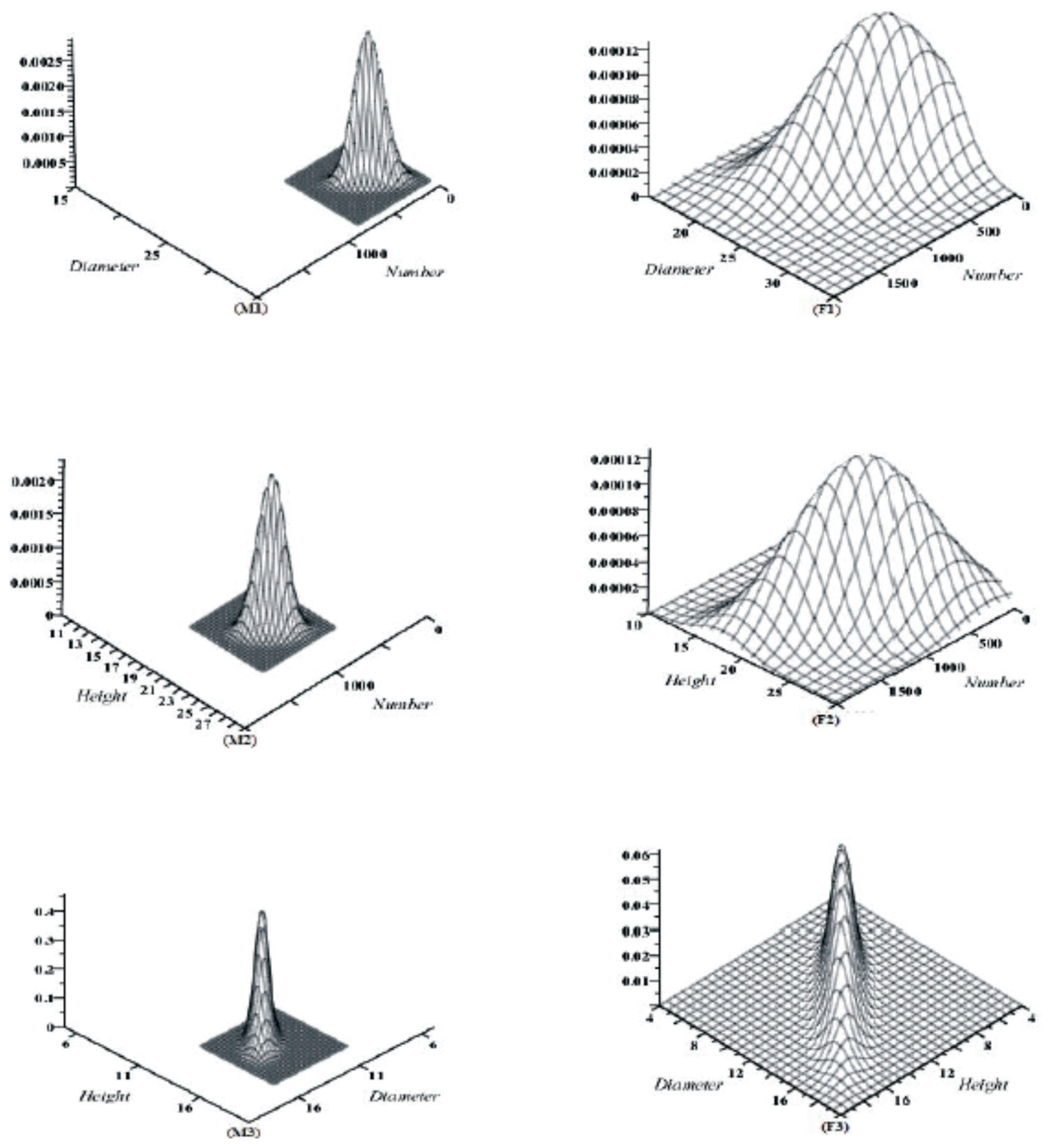
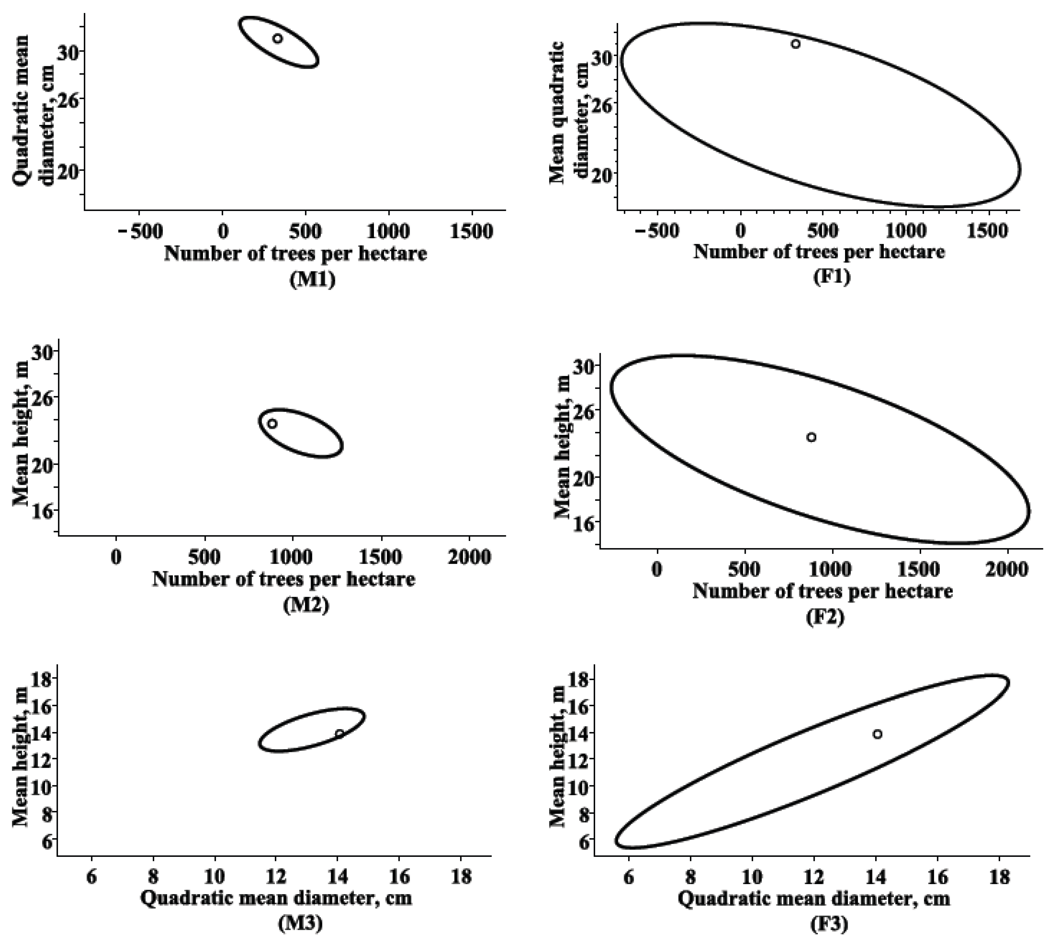
3.1. Marginal Bivariate Distributions

The focus of this study was mainly on the methodology of growth and yield modeling using a 3-variate SDE. The newly developed 3-variate probability density function defined by Equations (4)–(6) is reliable for its multiplicity of cases such as the marginal univariate and bivariate, and conditional univariate and bivariate probability density functions of the number of trees per hectare, quadratic mean diameter and mean height, and its global attractiveness in the context of the application perspective.
To demonstrate that the observed dataset of Scots pine trees does indeed follow the marginal bivariate estimated probability density function with the mean vector defined by Equation (7) and the covariance matrix defined by Equation (8), we used simple graphical techniques. In the sequel, the estimates of the fixed effect parameters θ f ^ and θ r ^ were calculated by the maximum likelihood procedure (see Table 1) using the estimation dataset (see Figure 1). In the forestry literature, calibration means that random effects are calibrated using a supplementary sample of observations taken from that sampling unit. The number of trees per hectare, quadratic mean diameter, and mean height could be predicted (forecasted) for the estimation (validation) dataset either by using random effects set to estimators determined by maximum likelihood procedure, or by using random effects that were calibrated from the previous observations { ( x 1 , 1 , x 2 , 1 , x 3 , 1 ) , ( x 1 , 2 , x 2 , 2 , x 3 , 2 ) , , ( x 1 , m , x 2 , m , x 3 , m ) } at discrete previous times (ages) { t 1 , t 2 , , t m } . The random effects ( ϕ 1 , ϕ 2 , ϕ 3 , ϕ 4 ) can be calibrated using the following form:
ϕ ^ = arg max ( ϕ 1 , ϕ 2 , ϕ 3 , ϕ 4 ) j = 1 m ln ( f ( x 1 , j , x 2 , j , x 3 , j , t j | θ r ^ , ϕ 1 , ϕ 2 , ϕ 3 , ϕ 4 ) ) + i = 1 4 ln ( p ( ϕ i | σ i ^ ) )
Figure 2 illustrates the estimated bivariate density functions with fixed effect- and mixed effect scenarios on three randomly selected stands at the ages t n i , i = 1, 2, 3, which correspond the observed validation dataset. The random effects were calibrated by Equation (15) using two previous observations at discrete times { t n i 1 , t n i 2 } , i = 1, 2, 3 from the estimation dataset. The estimated bivariate probability density functions presented in Figure 2 are flatter and the standard deviations are larger for the fixed-effect scenario, which most likely reflects the full-scale conditions of the temporal and spatial hierarchy dataset sampled. Figure 2 indicates that the fixed effect parameters bivariate density accounts for the range of size components variation in different stands. For mixed effect parameters scenario each stand size component variation should be expected to be peculiarly adapted to the stand variation.
The 95% confidence region plots of these estimated bivariate density functions and the observed data point from validation dataset are presented in Figure 3. The bivariate analog of confidence interval is given by an ellipsoid:
( x μ 2 , l ( t ) ) T [ Σ j k ( t ) ] 1 ( x μ 2 , l ( t ) ) = χ 2 2 ( α )
where 1 ≤ j, k ≤ 3, mean vector μ 2 , l ( t ) and covariance matrix Σ j k ( t ) are defined by Equations (7) and (8), respectively, and χ 2 2 ( α ) is from the Chi-square distribution with 2 degree of freedom. Specifically, if α = 0.05 ( χ 2 2 ( 0.05 ) 5.99 ), Equation (16) provides the confidence region containing 95% of the probability mass of the marginal bivariate distribution. Figure 3 shows that the mixed effect parameters bivariate estimated probability density function centered the observed data point better than the fixed effect parameters bivariate estimated probability density function for the three randomly selected stands from the validation dataset.
Figure 2 and Figure 3 show that the estimated mixed effect parameters bivariate probability density functions become steeper than fixed effects parameters densities. The 95% confidence regions of the estimated mixed effect parameters bivariate densities and the observed values given in Figure 3 show that the mixed effects model seems well capture the forthcoming values from the validation (forecast) dataset, but the fixed effects model shows worse results. Figure 3 illustrates negative correlations between mean tree size components and stand density and positive correlation between quadratic mean diameter and mean height.

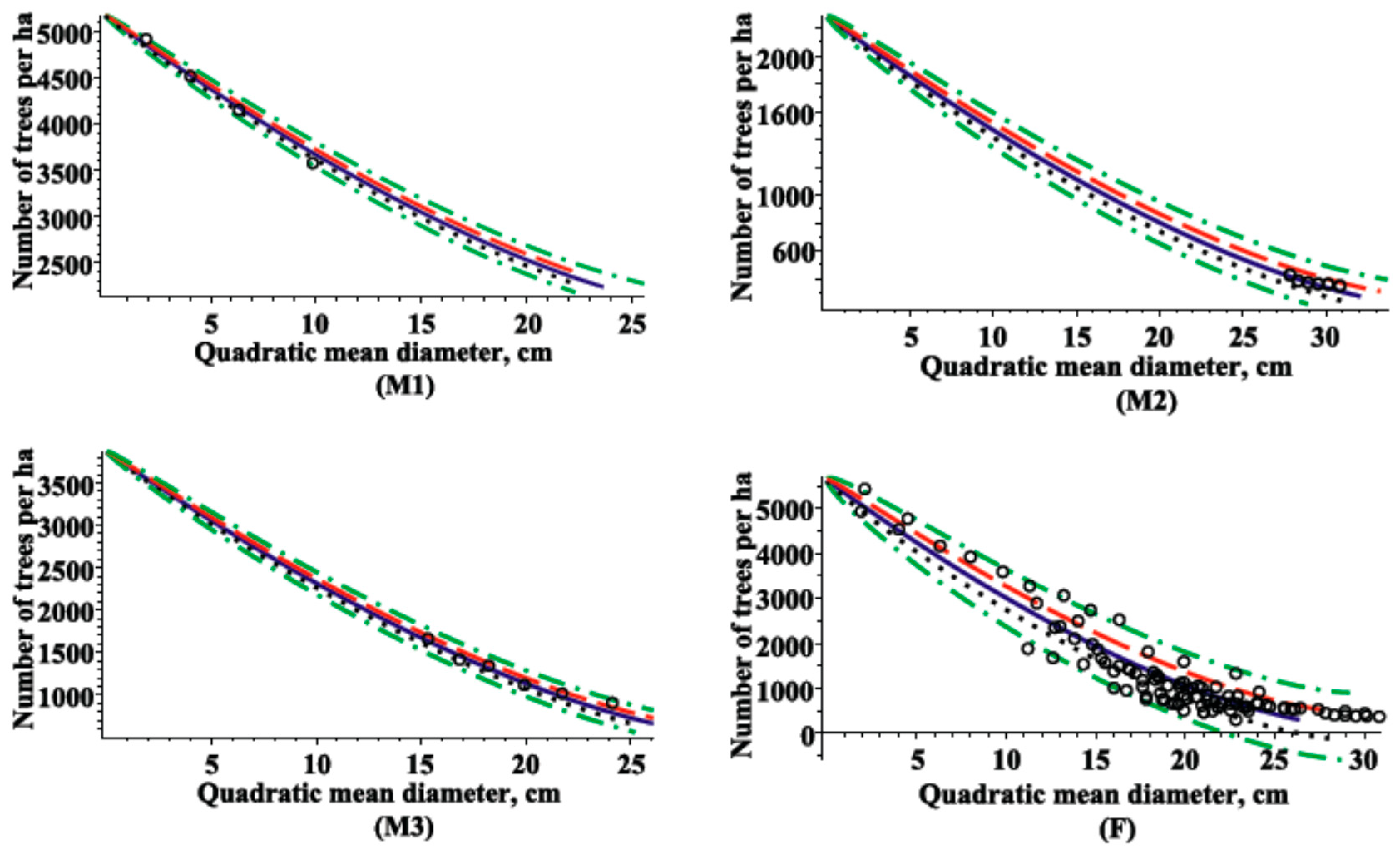
3.2. Maximum Density-Size Relationships

The number of trees per hectare varies with the quadratic mean diameter of the stand. Stands of small quadratic mean diameter have a large number of trees, while stands of large quadratic mean diameter have relatively few [20]. To develop the number of trees per hectare trajectory for all stands, it is necessary to determine a relationship describing development of the number of trees per hectare development versus the quadratic mean diameter [16,35,36]. The relationship between the quadratic mean diameter (increasing over age) and the number of live trees per hectare (decreasing over age) are commonly described by means of a “limiting relationship” [13]. In forest management interest has focused on how the quadratic mean diameter affects the tails of the conditional distribution of the number of trees per hectare [20,37]. Since the marginal univariate distribution of X i l ( t ) | X i l ( t 0 ) = x i 0 , i = 1, 2; l = 1, 2, …, M is the normal N 1 ( μ i l ( t ) ; v i i 2 ( t ) ) with mean and variance functions defined by Equations (4) and (5), it is possible to write the quantile equations (“limiting relationship”) of the number of trees per hectare and quadratic mean diameter subject to any desired conditional quantile, 0 < p < 1. Expressions for p-quantiles, 0 < p < 1, q x i l ( t , p ) , 1 i 2 , l = 1, 2, …, M can be formulated as follows:
q x 1 l ( t , p ) = Φ p 1 ( μ 1 l ( x ) ; ν 11 2 ( x ) )
q x 2 l ( t , p ) = Φ p 1 ( μ 2 l ( x ) ; ν 22 2 ( x ) )
A parametric representation of both (p,0.5)-quantile equations depending on the age as the parameter, { ( q x 2 l ( t , 0.5 ) , q x 1 l ( t , p ) ) , t = 10 , , 110 } , describes the maximum number (p-level quantile) of trees per hectare over the quadratic mean diameter. Figure 4 presents the fitted parametric equations involving the maximum number (p-level quantile) of trees per hectare over the quadratic mean diameter with five different p-quantile scenarios:
1)
{ ( q x 2 l ( t , 0.5 ) ,   q x 1 l ( t , 0.25 ) ) ,   t = 10 , , 110 } , lower quartile of stand density over quadratic mean diameter;
2)
{ ( q x 2 l ( t , 0.5 ) ,   q x 1 l ( t , 0.75 ) ) ,   t = 10 , , 110 } , upper quartile of stand density over quadratic mean diameter;
3)
{ ( q x 2 l ( t , 0.5 ) ,   q x 1 l ( t , 0.5 ) ) ,   t = 10 , , 110 } , mean of stand density over quadratic mean diameter;
4)
{ ( q x 2 l ( t , 0.5 ) ,   q x 1 l ( t , 0.95 ) ) ,   t = 10 , , 110 } , 95% percentile of stand density over quadratic mean diameter;
5)
{ ( q x 2 l ( t , 0.5 ) ,   q x 1 l ( t , 0.05 ) ) ,   t = 10 , , 110 } , 5% percentile of stand density over quadratic mean diameter.

4. Discussion

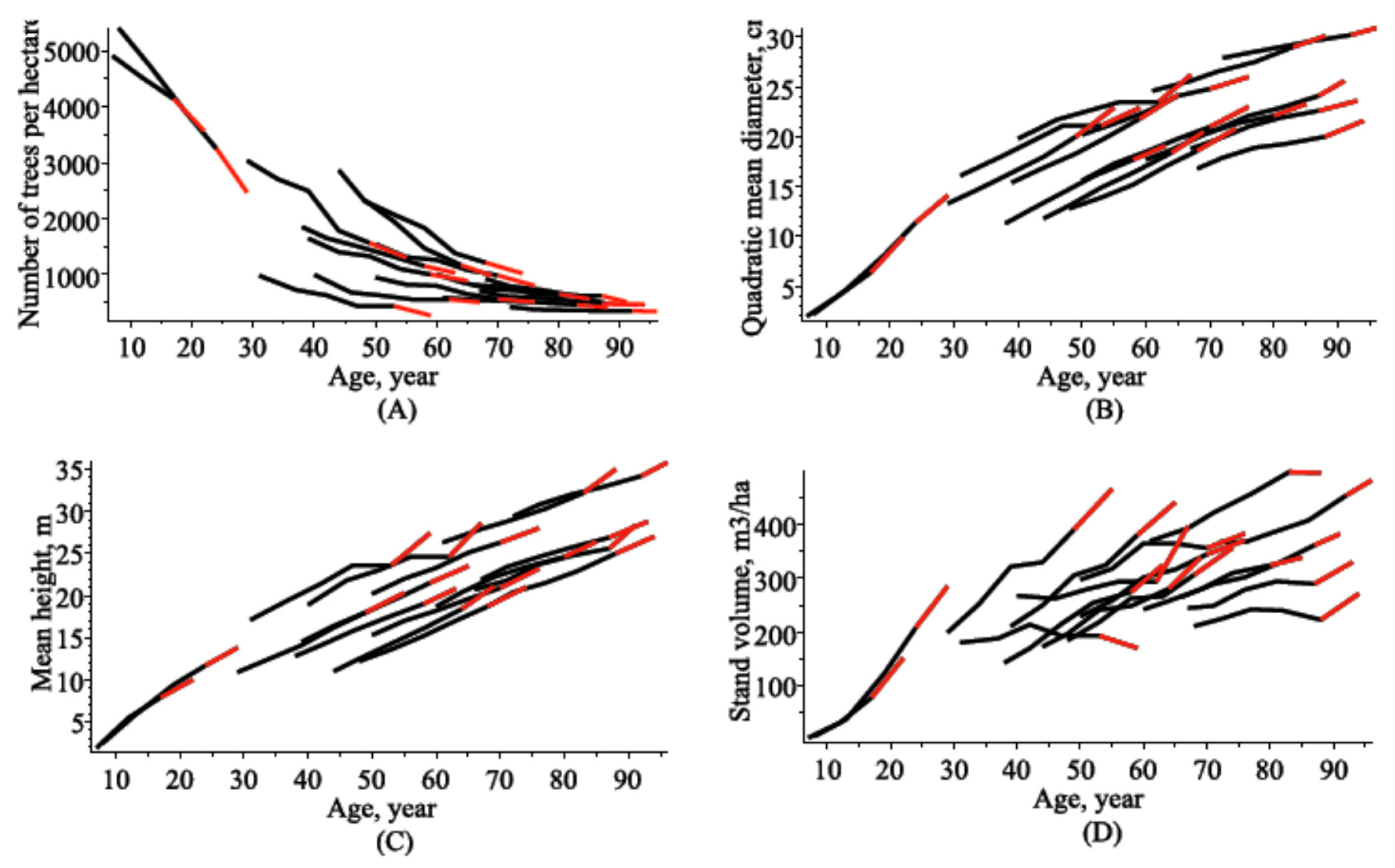
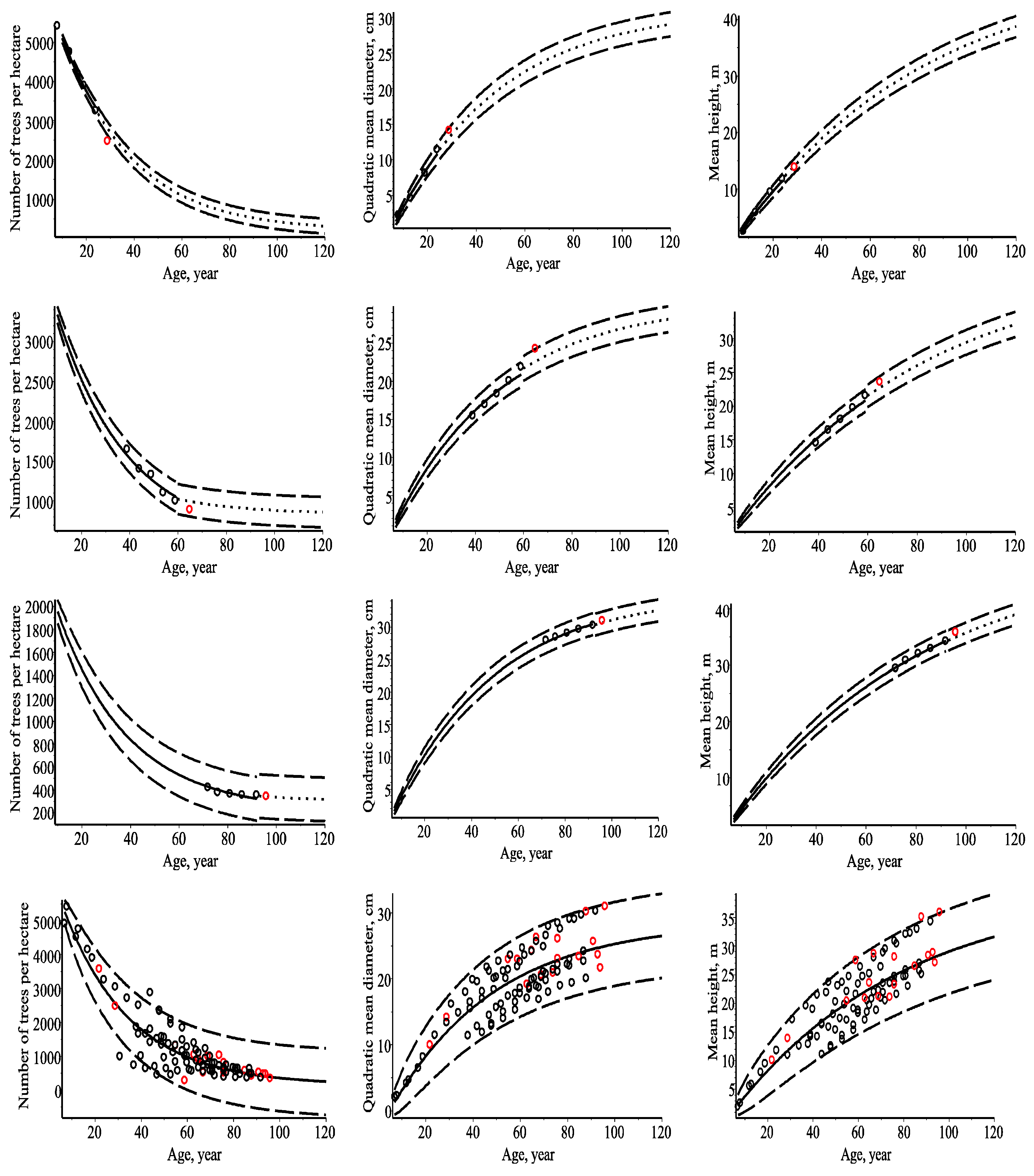
4.1. Models of the Number of Trees per Hectare, Quadratic Mean Diameter and Mean Height

Whole stand growth and yield modeling is still facing many challenges among which their complexity including interactions between various stand size components. This paper provides the state of art on advanced modeling on how stand size components (the number of trees per hectare, quadratic men diameter and mean height) interact. It is well-known that height growth is less sensitive to competition than diameter growth, so that height-diameter relationships vary depending on past stand densities [38]. This statement confirms that univariate stand size component relationships are unsatisfactory for the modeling of stand volume and biomass. The limitation of univariate methods for the frequency analysis of diameter (or height) has attracted the attention of foresters in recent decades [39,40]. Moreover, it is necessary to consider multivariate probability problems, since they can easily connect univariate marginal and conditional distribution probability density functions of stand density, quadratic mean diameter and mean height with their multivariate probability distributions.
Using univariate marginal probability densities, N 1 ( μ i l ( t ) , ν i i 2 ( t ) ) , i = 1, 2, 3, l = 1, 2, …, M with mean and variance defined by Equations (4) and (5) and the conditional probability densities, N 1 ( η i 2 , l ( t , x j , x k ) , λ i , 2 2 ( t ) ) , N 1 ( η i 1 , l ( t , x j ) , λ i , 1 2 ( t ) ) , with the mean and variance defined by Equations (10)–(14), respectively, we can predict (forecast) the response variable (the number of trees per hectare, quadratic mean diameter, and mean height) versus age and a given selection of one or two predictor variables. The number of trees per hectare, quadratic mean diameter, mean height, and basal area dynamics in the forestry literature have been formulated using a wide range of mathematical relationships from linearized fixed effect parameters regression equations to nonlinear mixed effect parameters generalized relationships [1,3,41]. The relationship between the quadratic mean diameter and the other stand variables such as the number of trees per hectare and mean height has many applications in forest inventory using remote sensing technologies [42].
In this study, the models concerning the dynamics of the number of trees per hectare, quadratic mean diameter, and mean height are listed by Equations (4), (10), and (12). Figure 5 shows the number of trees per hectare, quadratic mean diameter, mean height, and their 2 sigma limits dynamics via age for three randomly selected stands, using marginal univariate probability densities where mean and variance are defined by Equations (4) and (5) for both mixed- and fixed effects scenarios (the random effects were calibrated by Equation (15) using two previous observations at discrete times { t n i 1 , t n i 2 } , i = 1, 2, 3, from the estimation dataset). Plots presented in Figure 5 reveal the superiority of the mixed effects scenario to the fixed effects scenario. The mean curves of the number of trees per hectare, quadratic mean diameter and mean height for all stands in the validation dataset (see Figure 5) were clearly differentiated and each forecast curve was found passing really quite close to the measured point in the validation dataset. Except for some stands, which measurements passed 95% confidence limits of the mean trends (see Figure 5) for both fixed- and mixed effect scenarios. The 95% confidence limits generated for the mixed effects scenario showed that the quadratic mean diameter and mean height models complete cover both estimation and validation datasets.
Table 2 shows the fit statistics for both the estimation and validation datasets of the number of trees per hectare, quadratic mean diameter, mean height models, the p-value of the Shapiro-Wilk (1965) [43] normality test (SW-test) of the residuals, and the p-value of the Stjudent test (T-test) [44] for the difference between the mean value of model predictions (forecasts) and the mean observed value of experiment measurements, when the random effects were calibrated by Equation (15) using two previous observations at discrete times { t n i 1 , t n i 2 } , i = 1, 2, 3 from the estimation dataset. Table 3 shows the fit statistics and p-values of tests for both the estimation and validation datasets of the number of trees per hectare, quadratic mean diameter, mean height models using fixed effect parameters scenario. The Student (T)-test analyze whether the mean prediction (forecast) bias is excessively positive or excessively negative. It is understandable that what define small p-values of both statistics SW and T is relative to inherent variability of the estimation and validation datasets, and the more data we have the more certain we can be about the deviations.
Statistical indexes and p-values of both used tests presented in Table 2 and Table 3 reveal that mixed effect scenario framework outperformed fixed effects scenario. Therefore, from a statistical point of view (see Table 2; Table 3), for the impact on the number of trees per hectare, and quadratic mean diameter dynamics, mean height was revealed to be the most important predictor variable. For the impact on the mean height dynamic, quadratic mean diameter was revealed to be the most important predictor variable. For the mixed effects scenario forecast relationships of the number of trees per hectare, quadratic mean diameter and mean height attained acceptable values of statistical indexes and p-values of tests (see Table 2). For the fixed effects scenario, all forecast relationships attained lower values of statistical indexes and p-values of tests than the mixed effects scenario models (compare Table 2; Table 3).
For Scots pine stands the number of trees per hectare dynamic over dominant height was examined by Stankova (2016) [45] and attained the bias value −11.0 (−0.37%), the root mean square error value 403 and the coefficient of determination value 0.948. The transition functions method for the stand density predictions, using dataset from teak forests in southern India [46], produced coefficient of determination, 0.985, and root mean square error, 43.15. For Pinus radiata D. Don plantations in Galicia [9] explained 99.3% of the total variance. For the new developed mixed effects scenario stand density models the predictive ability accessed by statistical indexes such as the mean prediction bias (percentage), 0.352 (−0.06%), the root mean squared error of predictions (percentage), 45.173 (3.36%), the mean absolute prediction bias (percentage), 32.305 (3.32%), exceeds the results in previous studies [45].
Previous prediction models of quadratic mean diameter for Pinus radiata D. Don plantations in Galicia [9] attained coefficient of determination, 0.959, and root mean square error, 4.5 cm, and for teak forests in southern India [46] attained coefficient of determination, 0.742, and root mean square error, 2.3 cm. For Chinese pine (Pinus tabulaeformis) plantations situated on upland sites throughout northwestern Beijing the forecast model (5 year) attained coefficient of determination, 0.927 [47]. In this study, for the mixed effects scenario, the quadratic mean diameter prediction (forecast) defined by Equation (10) proved satisfactory with the mean prediction (forecast) bias, −0.001 cm (0.188 cm), the absolute prediction (forecast) bias, 0.266 cm (0.494 cm), the root mean squared prediction (forecast) error, 0.340 cm (0.469 cm), and prediction (forecast) coefficient of determination, 0.997 (0.992).

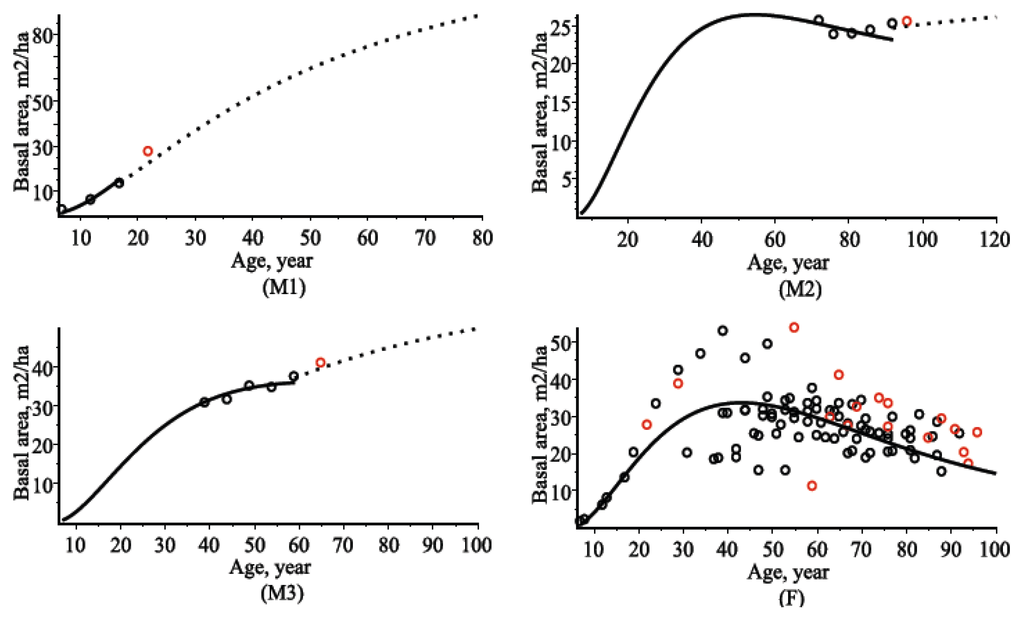
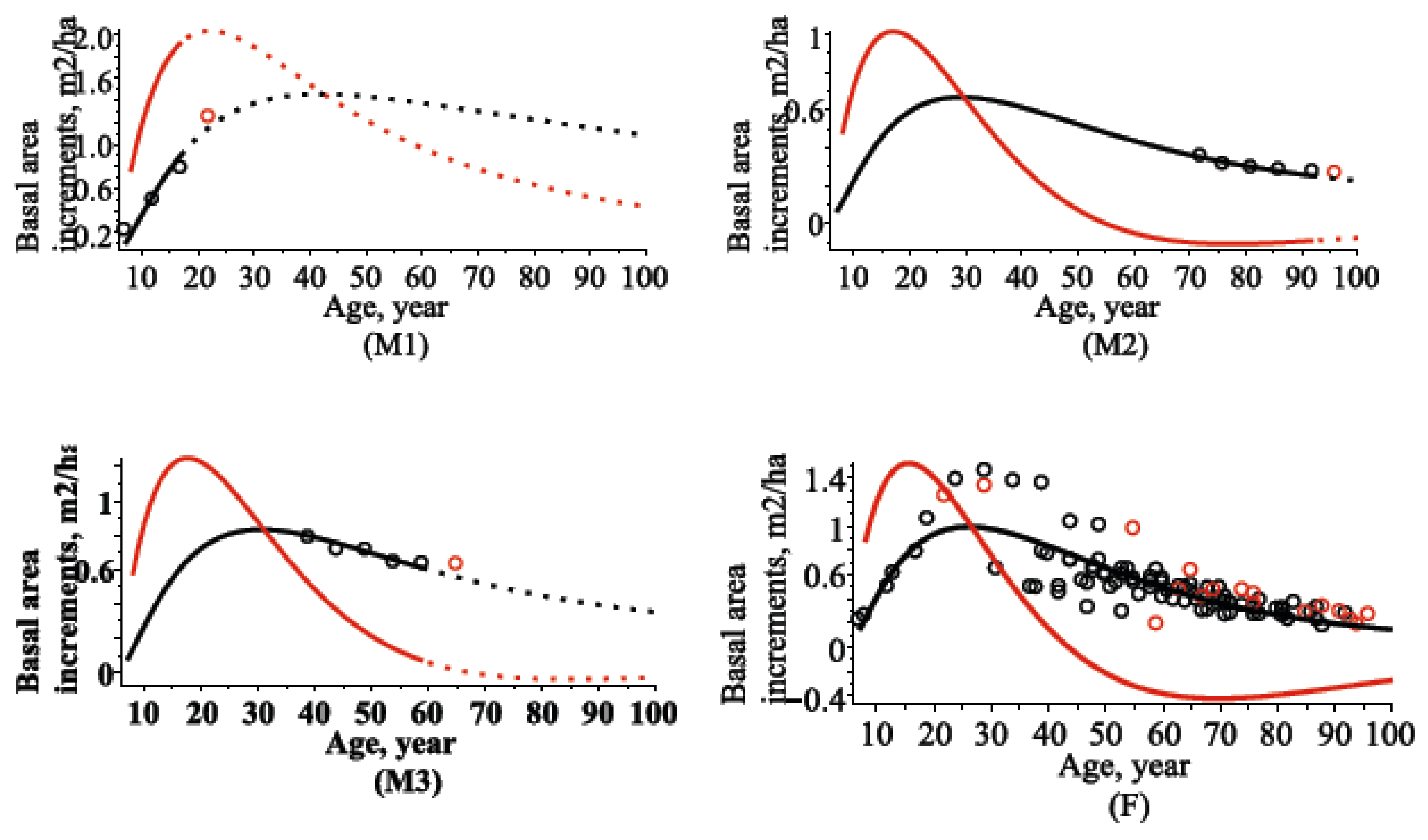
4.2. Stand Basal Area Models

Stand basal area, G, is an important variable of a forest stand which is simply the sum of the cross-sectional area at breast height of all trees per hectare of a forest stand (m2/ha). Stand basal area can be used to estimate stand volume or as a useful measure of the degree of competition in the stand [1,13]. Basal area growth describes the stand development over age and is traditionally used in exploring management scenarios [48]. Stand basal area is defined by:
G = π · D 2 40000 · N
By using the marginal bivariate (number of trees per hectare and quadratic mean diameter) probability density function defined by Equations (7) and (8), the basal area dynamic takes the following form:
G ( t ) = + + π · x 2 2 40000 · x 1 · f ( x 1 , x 2 | Θ ^ ) d x 1 d x 2 , Θ ^ { ( θ f ^ , 0 ) , ( θ r ^ , Ψ ^ ) }
Figure 6 represents the basal area dynamic over age with the observed dataset for three randomly selected stands using mixed effect scenario (the random effects were calibrated by Equation (15)) and for all stands using fixed effect scenario. Figure 6 illustrates that the mixed effects basal area relationship, defined by Equation (20), for three randomly selected stands provides the predicted (forecast) values closer to the observed stand basal area values than the fixed effects model.
Table 4 shows the goodness-of-fit statistics for stand basal area. From Table 4, it is clear that the mixed effect scenario model was more accurate in predicting (forecasting) stand basal area than the fixed effect scenario model.
Stand basal area modeling has a long history in forestry. In this study, for the mixed effects scenario the basal area per hectare defined by Equation (20) proved satisfactory with the mean prediction (forecast) bias, −0.115 m2 ha−1 (0.993 m2 ha−1), the absolute prediction (forecast) bias, 1.251 m2 ha−1 (2.028 m2 ha−1) and attained a high coefficient of determination, 0.968 (0.988). The combination modeling technique used to model stand basal area of Norway spruce [49] attained the coefficient of determination, 0.974, and the bias, 0.1 m2 ha−1. For loblolly pine (Pinus taeda L.) stands disaggregation modeling technique explained 86.2% of the total variance, attained the prediction bias 0.06 m2 ha−1 and the absolute prediction bias 2.17 m2 ha−1 [50].
Dynamic of a forest stand is a multiple process whose important stand level characteristic is biomass accumulation. Forest stand productivity is the production that can be realized at a certain site with a specified management regime. Assessment of the production capacity is necessary for the scientifically sound management. Stand basal area increment models are highly useful for estimation of the biomass production. The rate of increments could be ascertained either by systematic measurements of standing trees or by a stem analysis of felled trees. Using dynamical stand basal area growth model defined by Equation (20), we can define the current and mean annual basal area increments CAIG, MAIG, respectively, in the following forms:
C A I G ( t ) = d d t G ( t )
M A I G ( t ) = 1 t G ( t )
Relationships between basal area current and mean annual increments against the age of a forest stand are illustrated in Figure 7. As seen in Figure 7, the age of a stand exerts a strong influence on current and mean annual basal area increments. The effect of the age on basal area current annual increments becomes negligible above 100 years of age. From Figure 7, we can see that the culmination of the mean annual basal area increment is reached even later than that of the current annual increment. The peak in current and mean annual basal area increments occurred approximately at 20 and 30 years of age, respectively. The current annual basal area increment becomes equal to a mean annual increment at 30–45 years of age.

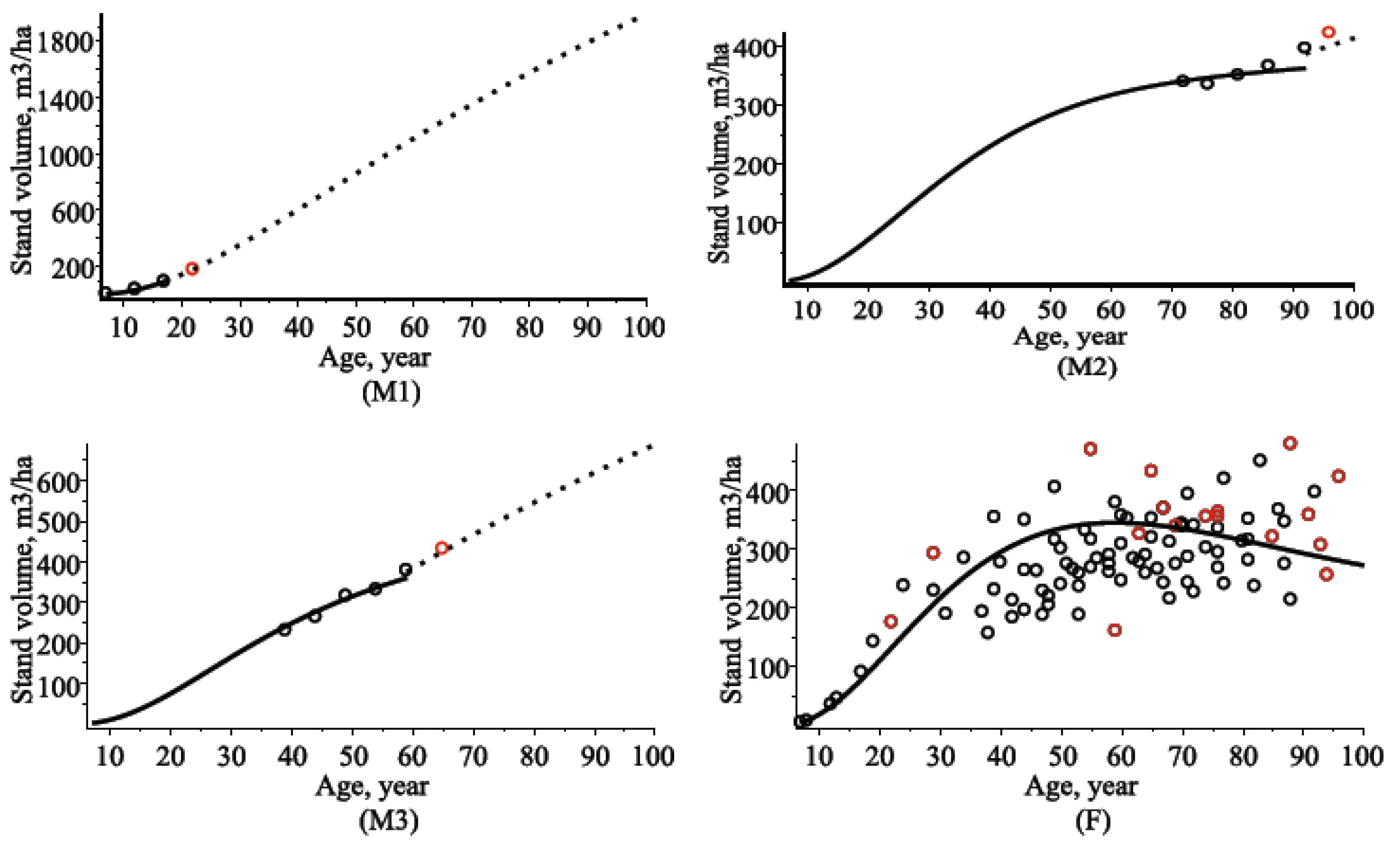
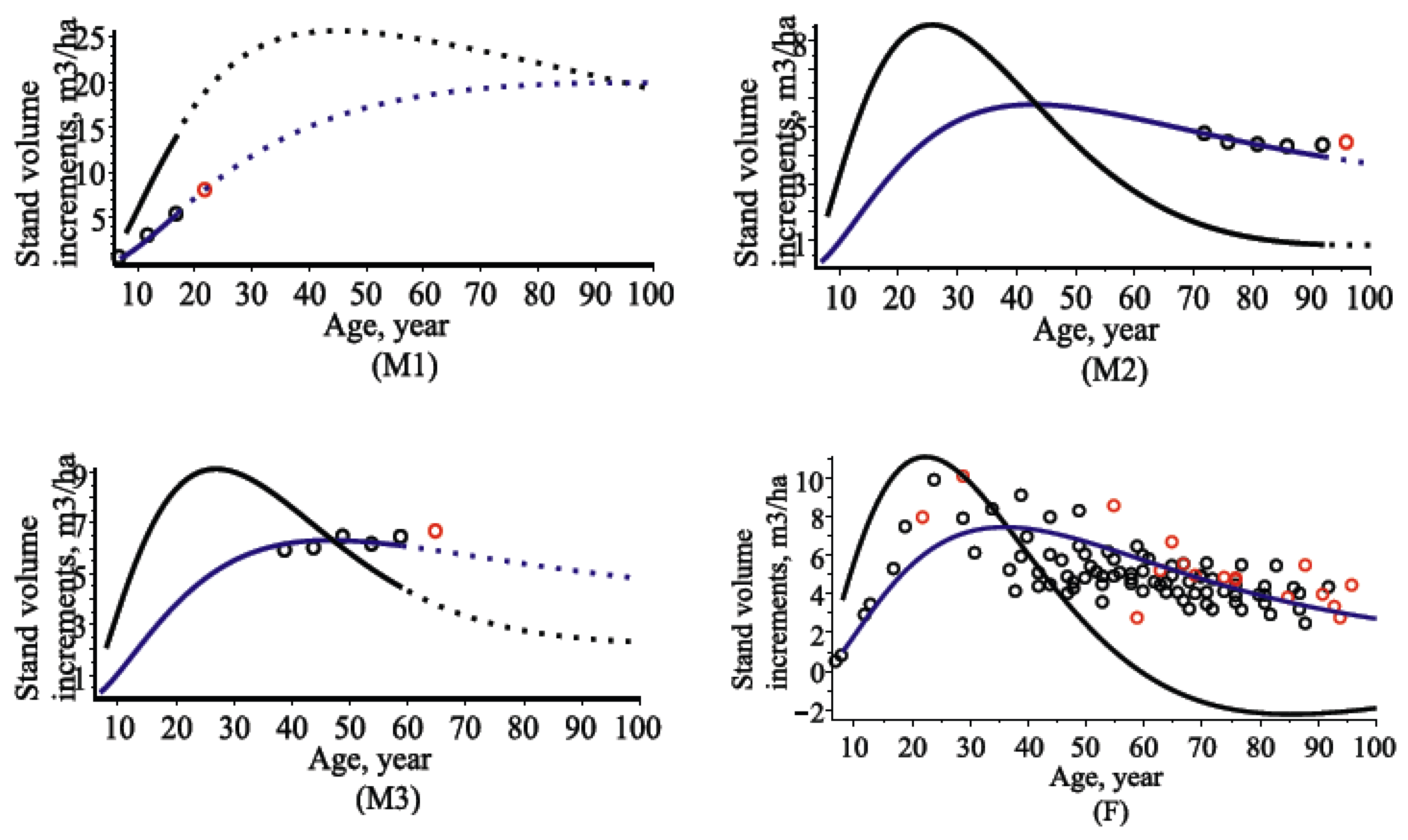
4.3. Stand Volume Models

The methodology of stand volume modeling is one of the main challenges in growth and yield forecasting [1]. The regression approach is traditionally used to estimate stand volume from measurements of more accessible variables such as the diameter at breast height and height that are measured directly in the Lithuanian National Forest Inventory (LNFI) [51]. This paper presents some current challenges, where multivariate SDEs have become a corner stone of whole stand growth modeling.
A typical example of a whole stand volume equation is given by [52,53]:
V S = G · H · F = π · D 2 40000 · N · H · F
Stand form factor, F, was estimated using observed datasets (see Figure 2) by a power regression equation in the following form:
F = F ( D , H ) = 1.4263 + D 1.0295 H 0.673
The trivariate probability density function, f ( x , y , z , t | θ , Ψ ) (number of trees per hectare, x, quadratic mean diameter, y, and mean height, z) defined by Equation (6) enables us to characterize a stand volume per hectare as a function of any specified stand age, t, in the following form:
V S ( t ) = π 40000 · + + + F ( y , z ) · x · y 2 · z · f ( x , y , z , t | Θ ^ ) · d x · d y · d z , Θ ^ { ( θ f ^ , 0 ) , ( θ r ^ , Ψ ^ ) }
Figure 8 shows the evolution of the stand volume per hectare as a function of a stand age using the fixed- and mixed effect scenarios. Table 5 shows the predictive ability for both newly developed fixed- and mixed effect scenarios stand volume per hectare models defined by Equation (25) for both estimation and validation (forecast) datasets using the estimates of parameters presented in Table 1. Naturally, the models of stand volume per hectare evolution show lower statistical indexes for the forecast (validation) dataset. The individually observed stand volume per hectare for all stands from the estimation and validation datasets were calculated by regression Equation (23). On the whole, for the mixed effects scenario, the stand volume per hectare defined by Equation (25) proved satisfactory with the percentage mean prediction (forecast) bias, −1.05% (5.47%), the percentage absolute prediction (forecast) bias, 5.338% (7.86%), the corrected root mean squared error of predictions (forecasts), 17.352 m3 ha−1 (30.276 m3 ha−1), and attained a high coefficient of determination of predictions (forecasts), 0.966 (0.980). Relative root mean squared error of stand volume predictions (forecasts) attained value 6.50% (8.93%). The inclusion of random effects in a trivariate SDE reduced the mean bias, mean absolute bias and root mean squared error of stand volume predictions (forecasts), and also increased the coefficient of determination.
According to the results presented by Stankova [45] for Scots pine stands, the best performing stand volume prediction model achieved prediction bias, −0.480 m3 ha−1 (–1.89%), the root mean squared prediction error, 41.81 m3 ha−1, and the coefficient of determination, 0.919. The Growfor (GF) dynamic empirical stand-level model based on the state-space framework [54] used to model stand volume of Sitka spruce (lodgepole) pine attained the relative mean prediction bias, −0.01–16.91% (−2.65–10.60%), the relative root mean squared error, 14.32–23.91% (14.33–29.13%), and the coefficient of determination, 0.62–0.92 (0.59–0.86). For teak forests in southern India [46] stand volume prediction models attained coefficient of determination, 0.97, and root mean square error, 13.34 m3 ha−1.
The stand volume curve defined by Equation (25) was used to define current annual increment (CAIV) and mean annual increment (MAIV) curves, respectively, in the following forms:
C A I V ( t ) = d d t V S ( t )
M A I V ( t ) = 1 t V S ( t )
CAIV is the yearly stand volume growth rate, while MAIV informs on the stand volume growth over the whole period from origin to a specific age. Together these curves inform the growth pattern of the forest stand and are of particular interest to forest managers, as the intersection of CAIV and MAIV curves informs on theoretical optimal harvest age that maximizes timber productivity [55]. Relationships between stand volume current and mean annual increments against the age of a forest stand are illustrated in Figure 9. As we see in Figure 9, the age of a stand exerts a strong influence on the current and mean annual stand volume increments. From Figure 9, we see that the culmination of the mean annual basal area increment is reached even later than that of the current annual increment. The peak in current and mean annual basal area increments occurred approximately at 20 and 30 years of age, respectively. The current annual basal area increment becomes equal to a mean annual increment at 30–45 years of age.

5. Conclusions

Growth processes in many areas of forestry, ecology, and environment are often perturbed by various types of environmental variation. In a general manner, eco-regional mixed effect parameters models are used as means to circumvent data collection and subsequent analyses. The essential features of the trees, the stands, and the way they change with age can be captured through growth and yield models by using the concept of diffusion processes. Most models of forest stand growth and yield are constructed from several equations independently fitted to datasets. Separate estimation of all model components increases overall model errors. This study focused on complex dynamical process defined by trivariate fixed-and mixed effect parameters Vašiček type SDE. Fundamental representation of a forest stand is formalized by the age-dependent trivariate probability density function of the number of trees per hectare, quadratic mean diameter, and mean height. New developed the mixed effect scenario SDE model relates the number of stems per hectare, quadratic mean diameter and mean height evolution to a mean stand age in the form of a trivariate age-dependent probability density function. This density function leads us to a variety of applications that span relationships of the most important stand characteristics such as the number of stems per hectare, quadratic mean diameter, mean height, basal area per hectare, stand volume per hectare, their increments and much more. The relationship of stand variable can be dependent on only stand age, or also on some predictors from a list defined by the number of stems per hectare, quadratic mean diameter and mean height. The newly developed model relates stand variables against the age dimension and consider the underlying covariance structure driving changes in the number of trees per hectare, quadratic mean diameter, and mean height. The views and results presented in this paper can be used for developing a new generation of stand growth and yield models. Using permanent sampling data of LNFI, the combination of those type of models with stem taper stochastic models [51] might be of interest in the wood industry. The potential wood consumer could get an output of the models, as detailed information on amounts of wanted sizes of roundwood.
Mixed effects SDE framework has made it possible to build dynamical models of structural components of forest stands from eco-regional databases like national inventory. Site quality variation can be accounted via random effect calibration (see, Equation (15)) using a sub-sample of trees measured for age, height, and breast height diameter.

Funding

This research received no external funding.

Acknowledgments

The author is grateful to two anonymous reviewers for handling the full submission of the manuscript.

Conflicts of Interest

The author declare no conflict of interest.

Appendix A. Maximum Likelihood Estimates

The SDE model defined by Equation (1) can be fitted to the number of trees per hectare (x1), quadratic mean diameter (x2), and mean height (x3) samples { ( x 1 , 1 l , x 2 , 1 l , x 3 , 1 l ) , ( x 1 , 2 l , x 2 , 2 l , x 3 , 2 l ) , , ( x 1 , n l l , x 2 , n l l , x 3 , n l l ) } at discrete times (ages) { t 1 l , t 2 l , , t n l l } (nl is the number of observed trees of the lth stand, l = 1 , 2 , , M ) by the maximum likelihood procedure. The associated maximum log-likelihood function for the 3-variate fixed effect SDE scenario takes the following form:
L L f ( θ f ) = l = 1 M j = 1 n l ln ( f ( x 1 , j l , x 2 , j l , x 3 , j l , t j l | θ f , 0 ) )
where θ f = { δ , α 1 , β 1 , α 2 , β 2 , α 3 , β 3 , σ 11 , σ 12 , σ 13 , σ 22 , σ 23 } are the fixed effects parameters (the same for all plots).
The maximum likelihood function for the 3-variate mixed effects SDE scenario takes the following form:
L r ( θ r , Ψ ) = l = 1 M + + + + j = 1 n l f ( x 1 , j l , x 2 , j l , x 3 , j l , t j l | θ r , ϕ 1 l , ϕ 2 l , ϕ 3 l , ϕ 4 l ) i = 1 4 p ( ϕ i l | σ i ) d ϕ 1 l ϕ 2 l d ϕ 3 l d ϕ 4 l
and the maximum log-likelihood function is:
L L r ( θ r , Ψ ) = l = 1 M + + + + ( j = 1 n l ln ( f ( x 1 , j l , x 2 , j l , x 3 , j l , t j l | θ r , ϕ 1 l , ϕ 2 l , ϕ 3 l , ϕ 4 l ) ) + i = 1 4 ln ( p ( ϕ i l | σ i ) ) ) d ϕ 1 l d ϕ 2 l d ϕ 3 l d ϕ 4 l
where θ r = { δ , α 1 , β 1 , α 2 , β 2 , α 3 , β 3 , σ 11 , σ 12 , σ 13 , σ 22 , σ 23 , σ 1 , σ 2 , σ 3 , σ 4 } are the fixed effects parameters (the same for all plots), Ψ = { ϕ 1 l , ϕ 2 l , ϕ 3 l , ϕ 4 l , l = 1 , 2 , , M } are random effects, ϕ 1 l , ϕ 2 l , ϕ 3 l , and ϕ 4 l are independent random variables (stand specific) following normal distributions with a 0 mean and constant standard deviations σ 1 , σ 2 , σ 3 , and σ 4 , respectively, and following the normal density functions p ( ϕ 1 l | σ 1 ) , p ( ϕ 2 l | σ 2 ) , p ( ϕ 3 l | σ 3 ) , and p ( ϕ 4 l | σ 4 ) , respectively.
As the 4-variate integral in Equation (A3) does not have a closed form solution and the analytic expression is known, so using the Laplace transform [56], the maximum log-likelihood function for the trivariate mixed effects SDE model is approximately given by:
L L r ( θ r , Ψ ^ ) l = 1 M ( g ( ϕ l ^ | θ r ) + 3 2 ln ( 2 π ) 1 2 ln ( det ( [ 2 g ( ϕ l | θ r ) ϕ j i ϕ k i ] ) ϕ l = ϕ l ^ ) )
The random effects ϕ l = ( ϕ 1 l , ϕ 2 l , ϕ 3 l , ϕ 4 l ) are estimated by maximization:
Ψ ^ = arg max ϕ l g ( ϕ l | θ r ^ ) ,   l = 1 , 2 , , M
where g ( ϕ l | θ r ) = j = 1 n l ln ( f ( x 1 , j l , x 2 , j l , x 3 , j l , t j l | θ r , ϕ l ) ) + i = 1 4 ln ( p ( ϕ i l | σ i ) ) .
The maximization of L L r ( θ r , Ψ ) is a two-step optimization problem. The internal optimization step estimates the vector ϕ l for every stand l = 1, 2, …, M with Equation (A5). The external optimization step maximizes L L r ( θ r , Ψ ^ ) after plugging the estimates ϕ l ^ into Equation (A4). These two steps are iterated until convergence.

References

  1. Burkhart, H.E.; Tomé, M. Modeling Forest Trees and Stands; Springer Science+Business Media: Dordrecht, The Netherlands, 2012. [Google Scholar]
  2. Hara, T. A stochastic model and the moment dynamics of the growth and size distribution in plant populations. J. Theor. Biol. 1984, 109, 173–190. [Google Scholar] [CrossRef]
  3. Vanclay, J.K. Tree diameter, height and stocking in even-aged forests. Ann. For. Sci. 2009, 66, 702. [Google Scholar] [CrossRef]
  4. Schwappach, A. Wachstum und Ertrag Normaler Fichtenbestände; Springer: Berlin, Germany, 1890. [Google Scholar]
  5. Guttenberg, A. Wachstum und Ertrag der Fichte im Hochgebirger; Wien: Leipzig, Germany, 1915. [Google Scholar]
  6. Assmann, E.; Franz, F. Vorläufige Fichten-Ertragstafel für Bayern. Forstwiss. Cent. 1965, 84, 13–43. [Google Scholar] [CrossRef]
  7. Curtis, R.O.; Marshall, D.D. Why quadratic mean diameter? West J. Appl. For. 2000, 15, 137–139. [Google Scholar]
  8. Newton, P. Stand density management diagrams: Review of their development and utility in stand–level management planning. For. Ecol. Manag. 1997, 98, 251–265. [Google Scholar] [CrossRef]
  9. Castedo-Dorado, F.; Crecente-Campo, F.; Álvarez-Álvarez, P.; Anta, M.B. Development of a stand density management diagram for radiata pine stands including assessment of stand stability. Forestry 2009, 82, 1–16. [Google Scholar] [CrossRef]
  10. Tewari, V.P.; Álvarez-Gonz, G. Development of a stand density management diagram for teak forests in southern India. J. For. Environ. Sci. 2018, 30, 259–266. [Google Scholar] [CrossRef]
  11. Garciá, O. Cohort aggregation modelling for complex forest stands: Spruce–aspen mixtures in British Columbia. Ecol. Model. 2017, 343, 109–122. [Google Scholar] [CrossRef]
  12. Cieszewski, C.J.; Balley, R.L. Generalized algebraic difference approach: Theory based derivation of dynamic site equations with polymorphism and variable asymptotes. For. Sci. 2000, 46, 116–126. [Google Scholar]
  13. Reineke, L.H. Perfecting a stand-density index for evenaged forests. J. Agric. Res. 1933, 46, 627–638. [Google Scholar]
  14. Lonsdale, W.M. The self–thinning rule: Dead or alive? Ecology 1990, 71, 1373–1388. [Google Scholar] [CrossRef]
  15. Pretzsch, H.; Biber, P. A re–evaluation of Reineke’s rule and stand density index. For. Sci. 2005, 51, 304–320. [Google Scholar]
  16. Vospernik, S.; Sterba, H. Do competition–density rule and selfthinning rule agree? Ann. For. Sci. 2014, 72, 379–390. [Google Scholar] [CrossRef]
  17. Yoda, K.; Kira, T.; Ogawa, H.; Hozumi, K. Self–thinning in overcrowded pure stands pure stands under cultivated and natural conditions. J. Biol. Osaka City Univ. 1963, 14, 107–129. [Google Scholar]
  18. Zeide, B. Analysis of the 3/2 power law of self-thinning. For. Sci. 1987, 33, 517–537. [Google Scholar]
  19. Ogawa, K.; Hagihara, A. Self–thinning and size variation in a sugi (Cryptomeria japonica D. Don) plantation. For. Ecol. Manag. 2003, 174, 413–421. [Google Scholar] [CrossRef]
  20. Clutter, J.L.; Bennett, F.A. Diameter Distributions in Old–Field Slash Pine Plantations; Georgia Forest Research Council: Atlanta, GA, USA, 1965.
  21. Cai, W.; Pan, J. Stochastic differential equation models for the price of European CO2 emissions allowances. Sustainability 2017, 9, 207. [Google Scholar] [CrossRef]
  22. Román-Román, P.; Serrano-Pérez, J.J.; Torres-Ruiz, F. Some notes about inference for the lognormal diffusion process with exogenous factors. Mathematics 2018, 6, 85. [Google Scholar] [CrossRef]
  23. Suzuki, T. Forest transition as a stochastic process. Mitt. Forstl. Bundesversuchsanstalt Wien 1971, 91, 69–86. [Google Scholar]
  24. Sloboda, B. Kolmogorow–Suzuki und die stochastische Differentialgleichung als Beschreibungsmittel der Bestandesevolution. Mitt. Forstl. Bundes-Versuchsanst. Wien 1977, 120, 71–82. [Google Scholar]
  25. Rupšys, P.; Petrauskas, E. Analysis of height curves by stochastic differential equations. Int. J. Biomath. 2012, 5, 1250045. [Google Scholar] [CrossRef]
  26. Rupšys, P. New insights into tree height distribution based on mixed effects univariate diffusion processes. PLoS ONE 2016, 11, e0168507. [Google Scholar] [CrossRef] [PubMed]
  27. Rupšys, P.; Petrauskas, E. A new paradigm in modelling the evolution of a stand via the distribution of tree sizes. Sci. Rep. 2017, 7, 15875. [Google Scholar] [CrossRef] [PubMed]
  28. Rupšys, P.; Petrauskas, E. A Linkage among tree diameter, height, crown base height, and crown width 4–variate distribution and their growth models: A 4–variate diffusion process approach. Forests 2017, 8, 479. [Google Scholar] [CrossRef]
  29. Rupšys, P.; Petrauskas, E. Evolution of bivariate tree diameter and height distribution via stand age: Von Bertalanffy bivariate diffusion process approach. J. For. Res. 2019, 24, 16–26. [Google Scholar] [CrossRef]
  30. Vasicek, O. An equilibrium characterization of the term structure. J. Financ. Econ. 1977, 5, 177–188. [Google Scholar] [CrossRef]
  31. Itô, K. On stochastic processes. Jpn. J. Math. 1942, 18, 261–301. [Google Scholar] [CrossRef]
  32. Tong, Y.L. The Multivariate Normal Distribution; Springer: New York, NY, USA, 1990. [Google Scholar]
  33. Linkevičius, E. Single Tree Level Simulator for Lithuanian Pine Forests. Ph.D. Thesis, Technische Universität Dresden, Tharandt, Germany, 2014. [Google Scholar]
  34. Monagan, M.B.; Geddes, K.O.; Heal, K.M.; Labahn, G.; Vorkoetter, S.M.; Mccarron, J. Maple Advanced Programming Guide; Maplesoft: Waterloo, ON, Canada, 2007. [Google Scholar]
  35. Ge, F.; Zeng, W.; Ma, W.; Meng, J. Does the slope of the self-thinning line remain a constant value across different site qualities?—An implication for plantation density management. Forests 2017, 8, 355. [Google Scholar] [CrossRef]
  36. Quiñonez-Barraza, G.; Ramírez-Maldonado, H. Can an exponential function be applied to the asymptotic density–size relationship? Two new stand-density indices in mixed–species forests. Forests 2019, 10, 9. [Google Scholar] [CrossRef]
  37. Mehtätalo, L.; Gregoire, T.G.; Burkhart, H.E. Comparing strategies for modeling tree diameter percentiles from remeasured plots. Environmetrics 2008, 19, 529–548. [Google Scholar] [CrossRef]
  38. Garciá, O. Reverse causality in size–dependent growth. Int. J. Math. Comput. For. Nat.-Resour. Sci. 2018, 10, 1–5. [Google Scholar]
  39. Ogana, F.N.; Osho, J.S.A.; Gorgoso-Varela, J.J. An approach to modeling the joint distribution of tree diameter and height data. J. Sustain. For. 2018, 37, 475–488. [Google Scholar] [CrossRef]
  40. Mulverhill, C.; Coops, N.C.; White, J.C.; Tompalski, P.; Marshall, P.L.; Bailey, T. Enhancing the estimation of stem–size distributions for unimodal and bimodal stands in a boreal mixedwood forest with airborne laser scanning data. Forests 2018, 9, 95. [Google Scholar] [CrossRef]
  41. McTague, J.P.; Weiskittel, A.R. Individual–tree competition indices and improved compatibility with stand–level estimates of stem density and long-term production. Forests 2016, 7, 238. [Google Scholar] [CrossRef]
  42. Humagain, K.; Portillo-Quintero, C.; Cox, R.D.; Cain, J.W. Mapping tree density in forests of the southwestern USA using landsat 8 data. Forests 2017, 8, 287. [Google Scholar] [CrossRef]
  43. Shapiro, S.S.; Wilk, M.B. An analysis of variance test for normality (complete samples). Biometrika 1965, 52, 591–611. [Google Scholar] [CrossRef]
  44. Dodge, Y. The Concise Encyclopedia of Statistics; Springer: New York, NY, USA, 2008; pp. 234–235. [Google Scholar]
  45. Stankova, T.V. A dynamic whole-stand growth model, derived from allometric relationships. Silva Fenn. 2016, 50, 1406. [Google Scholar] [CrossRef]
  46. Tewari, V.P.; Álvarez-González, J.G.; García, O. Developing a dynamic growth model for teak plantations in India. For. Ecosyst. 2014, 1, 9. [Google Scholar] [CrossRef] [Green Version]
  47. Zhang, X.; Lei, Y. A linkage among whole–stand model, individual tree model and diameter–distribution model. J. For. Sci. 2010, 56, 600–608. [Google Scholar] [CrossRef]
  48. Fu, L.; Sharma, R.P.; Zhu, G.; Li, H.; Hong, L.; Guo, H.; Duan, G.; Shen, C.; Lei, Y.; Li, Y.; et al. A basal area increment–based approach of site productivity evaluation for multi–aged and mixed forests. Forests 2017, 8, 119. [Google Scholar] [CrossRef]
  49. Yue, C.; Kohnle, U.; Hein, S. Combining tree and stand level models: A new approach to growth prediction. For. Sci. 2008, 54, 553–566. [Google Scholar]
  50. Cao, Q.V. Linking individual–tree and whole–stand models for forest growth and yield prediction. For. Ecosyst. 2014, 1, 1–8. [Google Scholar] [CrossRef]
  51. Petrauskas, E.; Bartkevičius, E.; Rupšys, P.; Memgaudas, R. The use of stochastic differential equations to describe stem taper and volume. Balt. For. 2013, 19, 43–151. [Google Scholar]
  52. Zianis, D.; Muukkonen, P.; Mäkipää, R.; Mencuccini, M. Biomass and stem volume equations for tree species in Europe. Silva Fenn. 2005, 4, 1–63. [Google Scholar]
  53. He, A.; McDermid, G.J.; Rahman, M.M.; Strack, M.; Saraswati, S.; Xu, B. Developing allometric equations for estimating shrub biomass in a Boreal Fen. Forests 2018, 9, 569. [Google Scholar] [CrossRef]
  54. McCullagh, A.; Black, K.; Nieuwenhuis, M. Evaluation of tree and stand–level growth models using national forest inventory data. Eur. J. For. Res. 2017, 136, 251–258. [Google Scholar] [CrossRef]
  55. Tompalski, P.; Coops, N.; White, J.; Wulder, M. Enhancing forest growth and yield predictions with airborne laser scanning data: Increasing spatial detail and optimizing yield curve selection through template matching. Forests 2016, 7, 255. [Google Scholar] [CrossRef]
  56. Picchini, U.; Ditlevsen, S.; De Gaetano, A. Practical estimation of high dimensional stochastic differential mixed–effects models. Comput. Stat. Data Anal. 2011, 55, 1426–1444. [Google Scholar] [CrossRef]
Figure 1. Observed datasets. Black–estimation dataset; red–validation dataset; (A) number of trees per hectare; (B) quadratic mean diameter; (C) mean height; (D) stand volume per hectare.
Forests 10 00506 g001
Figure 2. Estimated marginal bivariate density functions for three randomly selected stands. (M1M3) mixed effects scenario; (F1F3) fixed effects scenario; (M1F1) the first stand (age 96 years), quadratic mean diameter and number of trees per hectare; (M2F2) the second stand (age 65 years), mean height and number of trees per hectare; (M3F3) the third stand (age 29 years), mean height, and quadratic mean diameter.
Forests 10 00506 g002
Figure 3. The 95% confidence regions with the observed data point for three randomly selected: (M1M3) mixed effects scenario; (F1F3) fixed effects scenario; (M1,F1) the first stand, quadratic mean diameter and number of trees per hectare; (M2,F2) the second stand, mean height and number of trees per hectare; (M3,F3) the third stand, mean height, and quadratic mean diameter.
Forests 10 00506 g003
Figure 4. Relationships between the number of live trees per hectare (declining over age) and the quadratic mean diameter (increasing over age). (M1) mixed effects scenario for the first stand; (M2) mixed effects scenario for the second stand; (M3) mixed effects scenario for the third stand; (F) fixed effects scenario for all stands; solid-blue line—the third 0.5-quantile scenario; dash-red line—the second 0.75-quantile scenario; dot-black line—the first 0.25-quantile scenario; dashdot-green line—the 0.05-and 0.95-quantile scenarios; circle—observed values.
Forests 10 00506 g004
Figure 5. Mean of response variable dynamics and mean ± 2 standard deviations with observed data points. Mean response variable prediction trend from initial age to observed stand age—solid line and forecast trend from this age forward—dot line, for three randomly selected stands (from first till third row). First row—mixed effects scenario for the first stand; second row—mixed effects scenario for the second stand; third row—mixed effects scenario for the third stand; last row—fixed effects scenario for all stands; mean ± 2 standard deviations—dash; estimation dataset—black circles, validation dataset—red circles.
Forests 10 00506 g005
Figure 6. Evolution of basal area over age. (M1) mixed effects scenario for the first stand; (M2) mixed effects scenario for the second stand; (M3) left—mixed effects scenario for the third stand; (F) fixed effects scenario for all stands; black solid line—stand basal area prediction curve; black dot line—stand basal area forecast curve; black circles—estimation dataset, red circles—validation (forecast) dataset.
Forests 10 00506 g006
Figure 7. Evolution of current and mean annual basal area increments over age. (M1) mixed effects scenario for the first stand; (M2) mixed effects scenario for the second stand; (M3) mixed effects scenario for the third stand; (F) fixed effects scenario for all stands; black solid line—MAIG prediction curve; black dot line—MAIG forecast curve; red solid line—CAIG prediction curve; red dot line—CAIG forecast curve; black circles—estimation dataset, red circles—validation (forecast) dataset.
Forests 10 00506 g007
Figure 8. Evolution of stand volume per hectare over age. (M1) mixed effects scenario for the first stand; (M2) mixed effects scenario for the second stand; (M3) mixed effects scenario for the third stand; (F) fixed effects scenario for all stands; black solid line–stand volume prediction curve; black dot line–stand volume forecast curve; black circles–estimation dataset, red circles–validation (forecast) dataset.
Forests 10 00506 g008
Figure 9. Evolution of current and mean annual stand volume increments over age. (M1) mixed effects scenario for the first stand; (M2) mixed effects scenario for the second stand; (M3) mixed effects scenario for the third stand; (F) fixed effects scenario for all stands; black solid line-CAIV prediction curve; black dot line–CAIV forecast curve; blue solid line-MAIV prediction curve; blue dot line–MAIV forecast curve; black circles–estimation dataset, red circles–validation (forecast) dataset.
Forests 10 00506 g009
Table 1. Estimates of fixed effect parameters.
ScenarioParameters of drift term
α1β1α2β2α3β3δ
Fixed278.60.037828.530.022839.400.01365705.0
Mixed330.90.034328.590.022741.030.01285496.4
ScenarioParameters of diffusion term
σ11ρ12ρ13σ22ρ23σ33σ1σ2σ3σ3
Fixed12,765.0−0.5447−0.63270.41890.91040.3473----
Mixed625.3−0.7589−0.55720.03300.64120.0237435.74.2497.0471837.9
Table 2. Statistical indexes and p-values of the Shapiro-Wilk (SWp) and Student (Tp) tests for the mixed effect scenario models *.
(Equation):
(Predictors)
Estimation Dataset (Prediction)Validation Dataset (Forecast)
B
(%B)
PRAB
(%AB)
R2SW p
T p
B
(%B)
PRAB
(%AB)
R2SW p
T p
Number of trees per hectare
(4): (t)1.753
(–0.62)
75.9157.20
(5.45)
0.9960.090
0.989
−67.10
(–3.80)
132.03102.06
(11.68)
0.9820.650
0.750
(10): (d,h,t)0.352
(–0.06)
45.1832.31
(3.33)
0.9980.002
0.998
23.98
(8.05)
107.7773.09
(10.04)
0.9850.650
0.909
(13): (d,t)0.455
(−0.09)
46.0232.34
(3.38)
0.9980.002
0.997
21.37
(7.11)
101.0666.87
(9.02)
0.9870.018
0.919
(13): (h,t)0.704
(–0.21)
52.9536.78
(3.08)
0.9980.009
0.996
–8.79
(6.91)
140.0396.92
(12.77)
0.9730.047
0.967
Quadratic mean diameter
(4): (t)−0.012
(–0.18)
0.6690.531
(3.75)
0.9870.652
0.985
1.021
(5.01)
1.2121.069
(5.22)
0.9840.779
0.423
(10): (N,h,t)–0.001
(0.27)
0.3400.266
(2.03)
0.9970.980
0.998
0.371
(1.66)
0.5980.494
(2.34)
0.9920.779
0.769
(13): (N,t)−0.002
(0.03)
0.4100.318
(1.99)
0.9950.906
0.997
0.598
(2.38)
0.9220.771
(3.59)
0.9810.619
0.636
(13): (h,t)−0.004
(0.39)
0.3870.309
(2.94)
0.9960.688
0.994
0.400
(2.54)
0.7580.571
(3.21)
0.9900.835
0.751
Mean height
(4): (t)−0.008
(–0.84)
0.6530.495
(3.36)
0.9910.059
0.992
1.045
(3.83)
1.3171.154
(4.80)
0.9850.440
0.525
(10): (N,d,t)−0.002
(–0.74)
0.3490.256
(2.37)
0.9970.133
0.998
0.399
(0.67)
0.8940.765
(3.61)
0.9850.440
0.807
(13): (N,t)−0.002
(–0.72)
0.4440.342
(2.74)
0.9960.435
0.998
0.746
(1.93)
1.3091.127
(5.17)
0.9740.036
0.649
(13): (d,t)–0.002
(−0.76)
0.3590.268
(2.42)
0.9970.349
0.998
0.377
(0.69)
0.8140.700
(3.26)
0.9880.198
0.817
* The best values of the statistical indexes are in bold, the mean prediction bias ( B = 1 n i = 1 n ( y i y i ^ ) ) and the percentage mean prediction bias ( % B = 1 n i = 1 n y i y i ^ y i · 100 ), the absolute mean prediction bias ( A B = 1 n i = 1 n | y i y i ^ | ) and the percentage mean absolute prediction bias ( % B = 1 n i = 1 n | y i y i ^ y i | ), an adjusted root mean square error ( P R = B 2 + 1 n 1 i = 1 n ( y i y i ^ B ) 2 ) and coefficient of determination ( R 2 = 1 i = 1 n ( y i y i ^ ) 2 i = 1 n ( y i y ¯ ) 2 ). Here n = i = 1 M n i is the total number of observations used to fit (forecast) the model, M is the number of stands, ni is the number of measured trees in the ith stand, y i , y i ^ and y ¯ are the measured, estimated, and average values of the dependent variable (number of trees per hectare, N, quadratic mean diameter, d, or mean height, h, stand basal area, G, stand volume, VS).
Table 3. Statistical indexes and p-values of the Shapiro-Wilk (SWp) and Student (Tp) tests for the fixed effect scenario models *.
(Equation):
(Predictors)
Estimation Dataset (Prediction)Validation Dataset (Forecast)
B
(%B)
PRAB
(%AB)
R2SW p
T p
B
(%B)
PRAB
(%AB)
R2SW p
T p
Number of trees per hectare
(4): (t)21.52
(−15.22)
465.27327.35
(33.99)
0.8330.143
0.864
10.43
(−16.97)
259.95174.54
(32.12)
0.9070.117
0.960
(10): (d,h,t)13.52
(−4.37)
304.47223.59
(23.27)
0.9290.296
0.915
121.51
(15.58)
222.52157.51
(27.24)
0.9520.117
0.565
(13): (d,t)17.02
(−7.19)
359.18269.73
(28.24)
0.9010.586
0.893
111.22
(5.34)
271.51213.08
(36.72)
0.9160.496
0.598
(13): (h,t)14.71
(−4.35)
306.04224.67
(23.32)
0.9320.223
0.907
124.60
(15.81)
224.99159.99
(27.63)
0.9520.101
0.556
Quadratic mean diameter
(4): (t)0.066
(−2.32)
3.1712.697
(14.90)
0.7120.0004
0.919
1.342
(5.14)
3.0992.508
(10.68)
0.7010.582
0.295
(10): (N,h,t)0.004
(0.13)
1.0690.877
(6.33)
0.9670.048
0.995
0.098
(0.34)
1.5011.096
(4.90)
0.9140.740
0.937
(13): (N,t)0.009
(−0.43)
2.4322.014
(11.87)
0.8310.013
0.989
1.373
(5.97)
2.8502.223
(9.95)
0.7610.708
0.284
(13): (h,t)0.008
(0.21)
1.0750.880
(6.25)
0.9670.024
0.990
0.104
(0.43)
1.5061.091
(4.84)
0.9130.719
0.934
Mean height
(4): (t)−0.087
(−3.46)
3.4792.872
(15.41)
0.7330.0004
0.906
1.515
(4.92)
3.7582.698
(10.32)
0.7300.147
0.359
(10): (N,d,t)0.0004
(−0.80)
0.9410.805
(5.65)
0.9800.004
0.999
0.333
(0.90)
1.6171.315
(5.40)
0.9430.840
0.838
(13): (N,t)‒0.0006
(−1.14)
2.3041.874
(11.29)
0.8833.9 × 10−5
0.999
1.545
(6.05)
3.1032.245
(9.19)
0.8350.106
0.350
(13): (d,t)−0.019
(−1.26)
1.1610.977
(6.58)
0.9700.064
0.976
0.196
(0.08)
1.7791.376
(5.49)
0.9290.976
0.904
* The best values of the statistical indexes are in bold.
Table 4. Statistical indexes and p-values of the Shapiro-Wilk (SWp) and Student (Tp) tests for the basal area (m2 ha−1) Equation (20) *.
ScenarioEstimation Dataset (Prediction)Validation Dataset (Forecast)
B
(%B)
PRAB
(%AB)
R2SW p
T p
B
(%B)
PRAB
(%AB)
R2SW p
T p
Mixed−0.115
(−0.30)
1.7601.251
(6.23)
0.9680.097
0.907
0.993
(3.80)
2.7332.028
(7.38)
0.9880.580
0.678
Fixed−0.746
(−8.08)
6.9174.972
(20.70)
0.5100.098
0.452
4.352
(4.67)
9.5687.081
(27.70)
0.8670.104
0.082
* The best values of the statistical indexes are in bold.
Table 5. Statistical indexes and p-values of the Shapiro-Wilk (SWp) and Student (Tp) tests for the stand volume (m3 ha−1) model (Equation (25)) *.
ScenarioEstimation Dataset (Prediction)Validation Dataset (Forecast)
B
(%B)
PRAB
(%AB)
R2SW p
T p
B
(%B)
PRAB
(%AB)
R2SW p
T p
Mixed−0.323
(−1.05)
17.35512.016
(5.33)
0.9660.008
0.973
19.281
(5.47)
35.89426.235
(7.86)
0.9800.028
0.381
Fixed−12.971
(−9.39)
62.40350.605
(20.87)
0.5830.360
0.176
57.935
(11.98)
97.90178.597
(24.49)
0.8620.119
0.015
* The best values of the statistical indexes are in bold.

