Abstract
Urban forests are an important component of the urban ecosystem. Urban forest types are a key piece of information required for monitoring the condition of an urban ecosystem. In this study, we propose an urban forest type discrimination method based on linear spectral mixture analysis (LSMA) and a support vector machine (SVM) in the case study of Xuzhou, east China. From 10-m Sentinel-2A imagery data, three different vegetation endmembers, namely broadleaved forest, coniferous forest, and low vegetation, and their abundances were extracted through LSMA. Using a combination of image spectra, topography, texture, and vegetation abundances, four SVM classification models were performed and compared to investigate the impact of these features on classification accuracy. With a particular interest in the role that vegetation abundances play in classification, we also compared SVM and other classifiers, i.e., random forest (RF), artificial neural network (ANN), and quick unbiased efficient statistical tree (QUEST). Results indicate that (1) the LSMA method can derive accurate vegetation abundances from Sentinel-2A image data, and the root-mean-square error (RMSE) was 0.019; (2) the classification accuracies of the four SVM models were improved after adding topographic features, textural features, and vegetation abundances one after the other; (3) the SVM produced higher classification accuracies than the other three classifiers when identical classification features were used; and (4) vegetation endmember abundances improved classification accuracy regardless of which classifier was used. It is concluded that Sentinel-2A image data has a strong capability to discriminate urban forest types in spectrally heterogeneous urban areas, and that vegetation abundances derived from LSMA can enhance such discrimination.
1. Introduction
Urban forests are important carriers of urban ecosystems [1,2], which can improve the urban microclimate, maintain the surface water–heat exchange balance [3,4], mitigate rainstorm runoff [5,6], and provide a comfortable habitat for urban residents [7]. Discriminating urban forest types has fundamental implications for planning, management, and protection of urban forests, as well as for forestry studies [8]. It also provides a basis for the estimation of above-ground biomass of urban vegetation [9,10]. Since it was first introduced by Jorgensen (1986) [11], urban forestry received increasing attention from scholars. However, the scope of urban forests was defined from a variety of research perspectives [12,13,14]. An urban forest can refer to all the trees in an urban area, including forest parks, and public and private woodlands [15], while Miller (1996) [16] and other researchers [17,18] consider urban forests as the sum of all the vegetation in the city, not only trees, but also park vegetation and private vegetation. In this study, we adopt the broader definition given by Miller—who also uses urban vegetation and urban forests interchangeably—and refer to an urban forest as a sum of trees in groups or individual trees, shrubs, and grassland within an urban area. Previous studies on urban forests focused on their release of oxygen and carbon [19], cooling and humidification effects [20], and landscape patterns [21,22]. However, discrimination of urban forest types was little studied despite being considered essential for urban forestry.
Field-based inventorying is the traditional and the most accurate method for vegetation survey and monitoring [23], but its use is restricted because it is time-consuming, expensive, and slow in updating [22]. As such, a quick and reliable approach is needed, which now can be addressed by applying remote-sensing (RS) technology. RS provides multi-source earth observation data at varying spatial resolutions from repeated visits, which allows forests to be surveyed and mapped rapidly and dynamically [24]. Based on the source of data used, an RS classification-based discrimination approach can be roughly divided into two categories [8]. One involves urban forest vegetation classification based on optical remote-sensing data, including moderate-resolution Landsat TM (Thematic Mapper)/ETM+ (Enhanced Thematic Mapper Plus) and AVIRIS (Airborne Visible/Infrared Imaging Spectrometer) imagery [25,26,27], and (very) high-resolution IKONOS, Worldview, airborne, and UAV (Unmanned Aerial Vehicle) imagery [28,29,30,31]; the other involves making use of radar data (including spaceborne and airborne radar) [32,33,34,35]. Some researchers also worked on an integrated use of these multi-source remote-sensing data for discriminating urban forest types [36]. Dalponte et al. (2012) [8] combined very-high-resolution multispectral/hyperspectral imagery and LiDAR (Light Detection and Ranging) data to classify forest vegetation in the Southern Alps, and distinguished five forest types. Liu et al. (2017) [37] identified 15 urban vegetation species types based on an aeronautical hyperspectral and airborne LiDAR point cloud. These studies used either free relatively coarse-resolution image data or purchased high-resolution image data, but none took advantage of the latest free multispectral image data with increased spatial resolution, such as Sentinel-2A.
It is noted that, because urban forests are often disturbed by human activity and, in a spectrally heterogeneous urban context, do not spread continuously like natural forests, it is challenging for traditional supervised classification methods to acquire highly separable training samples and get a satisfying classification accuracy of urban forest type discrimination [38]. Linear spectral mixture analysis (LSMA)—which is frequently used for estimating spectral endmember abundances from hyper- or multispectral images—offers an alternative to obtaining training samples for classifying urban vegetation [39,40]. In addition, machine learning algorithms such as support vector machines (SVM) and random forests (RF) can extract effective features from large feature datasets and produce higher classification accuracy than ordinary maximum-likelihood and K-means classifiers [41,42]. These promise a possible improvement in urban forest mapping and discrimination.
In order to contribute to the general objective of estimating the above-ground biomass in urban areas, this study assesses the possibility of mapping urban forest types from a single Sentinel-2A image. We, therefore, propose in this study an innovative method by combing linear spectral mixture analysis (LSMA) and an SVM machine learning algorithm in Xuzhou, east China. Specific objectives were (1) to investigate the capability of Sentinel-2A data and LSMA for extracting urban forest vegetation endmembers; (2) to find out the optimal feature combination for mapping urban forests; and (3) to identify whether vegetation abundances are similarly effective in improving classification accuracy when different machine learning classifiers are performed.
2. Study Area and Data
2.1. Study Area
Bordering the provinces of Shandong, Henan, and Anhui in a counterclockwise direction, Xuzhou (33°43′–34°58′ north (N), 116°22′–118°40′ east (E)) is located in the northwestern part of Jiangsu province with an average altitude below 400 m (Figure 1). It has a warm temperate semi-humid monsoon climate and a frost-free period of 200–220 days, with an average annual temperature of 13–16 °C and an average annual precipitation of 800–900 mm [43]. In 2017, the forest coverage area of Xuzhou was 336,300 ha—a forest coverage rate as high as 30.12%, which ranked Xuzhou first in Jiangsu. It is one of the “National Forest Cities” (awarded in 2012) and the “National Ecological Garden Cities” (awarded in 2016).
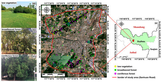
Figure 1.
The location of the study area: (a–c) field photos illustrating three different urban forest types; (d) sites for field investigation (yellow for low vegetation, green for broadleaved forest, and purple for coniferous forest), the border of the study area, and a true-color composition of the Sentinel-2A image used for classification. Labels ①–④ refer to the hills of Zhushan, Yunlong, Zifang, and Jiuli, respectively; (e) study area in Xuzhou.
The study area is within the Sanhuan Road of Xuzhou, covering an area of approximately 108.51 km2. The northern, eastern, and southern parts of the study area are hilly lands (labeled ①–④ in Figure 1d), dominantly covered by Platycladus orientalis (L.) Franco, whereas the central part is for commercial and residential purposes. Based on our prior knowledge coupled with field observations, urban forests in the study area were concentrated and tended to be fragmented. Different vegetation types exist mostly independent of each other. Therefore, we divided the land cover of the study area into five types: broadleaved forest, coniferous forest, low vegetation (including shrubs, grasslands, and suburban farmlands), water bodies, and non-vegetation area (excluding water bodies).
2.2. Data
2.2.1. Satellite Data
Data used for mapping and discriminating urban forest types involved a single Sentinel-2A image acquired on 24 July 2017 with little cloud contamination (1.74%) and downloaded from the Copernicus Open Access Hub (https://scihub.copernicus.eu/dhus/#/home). The Sentinel-2 satellite was launched by the European Space Agency (ESA) in mid-2015 aimed at earth observation. It travels in a sun-synchronous orbit with an orbit height of 786 km and an inclination angle of 98.5°, providing image data of 290 km in width [44]. The Sentinel-2A satellite carries a multispectral instrument (MSI), providing a total of 13 bands from visible light to shortwave infrared (four bands at 10 m, six bands at 20 m, and three bands at 60 m; for more details about Sentinel-2A bands, please refer to the overview introduction of Sentienl-2 MSI images on the website of the ESA [45]).
Compared with Landsat and SPOT (Systeme Probatoire d’Observation de la Terre) data, Sentinel-2 images have more advantages in discriminating urban forest types due to their increased multispectral bands, increased spatial resolution, and shorter revisit period [46,47]. They are characterized by three unique “vegetation red-edge” bands (bands 5, 6, and 7), which are valuable for remote sensing of vegetation. Although it was widely used in the monitoring of fires [48], vegetation biophysical estimation [49,50], and surface feature extraction analysis [51], the potential of Sentinel-2 data to discriminate urban forest types remains to be fully acknowledged.
The product level of the Sentinel-2A image used in this study was Level-1C, which means that geometric correction, radiation calibration, and top of atmosphere (TOA) correction were already applied [52].
Preprocessing of Sentinel-2A Level-1C products includes atmospheric correction, resampling, and clipping. The atmospheric correction was conducted in the Sen2cor plugin, a Python-based atmospheric correction tool used in SNAP® (Sentinel Application Platform), which is an open-source application developed by ESA for processing Sentinel-1 to -3 data and is freely available from ESA’s website. Through atmospheric correction, the Level-1C data were converted into Level-2A data, such as bottom of atmosphere (BOA), aerosol optical thickness images, and water vapor images [52]. In our study, 10-m bands and 20-m bands were independently corrected before the 20-m bands were resampled to 10-m bands using the nearest neighbor method in SNAP. In total, ten bands were used, except for bands 1, 9, and 10, because they are not relevant to vegetation. Clipping (i.e., extracting the study area from the image) and other data processing (e.g., layer stacking and spectral mixture analysis) were done in ENVI® (remote sensing software by US-based Harris Geospatial Solutions. Inc., Broomfield, Colorado, CO, USA).
2.2.2. Fieldwork
In order to identify forest types on the field and collect validation data for image classification accuracy assessment, we conducted fieldwork from October to December 2017. Despite being three months later than the acquisition data of the Sentinel-2A image, this is considered acceptable for a study area where vegetation does not change much over three months.
A total of 192 sites for fieldwork were randomly selected on the corrected Sentinel-2A image (Universal Transverse Mercator Projection WGS84-50N) in ArcGIS® (geographic information system software by US-based Esri Inc., Redlands, CA, USA). Then, we localized these pre-selected sites on the field using hand-held Hi-Target® Hi-Q5 GPS devices (by China-based Hi-Target Surveying Instrument Co. Ltd, Guangzhou, China), which have a maximal horizontal accuracy of 0.5 m when connected with the continuously operating reference stations (CORS) network of Xuzhou. Due to restricted accessibility of some areas in Xuzhou (such as special education schools, military zones), the number of effective sites was 140 (35 coniferous forest sites, 73 broadleaved forest sites, and 32 low vegetation sites; see Table A1, Appendix A), down from the pre-selected 192.
On the field, we recorded tree species and other parameters, such as tree height, diameter at breast height (DBH), crown width, and vegetation coverage for our further research on urban biomass estimation, within a 10 m × 10 m rectangle centered at the site’s coordinates. The size of the rectangle allows a spatial match with a Sentinel-2A pixel.
3. Methods
A technical flowchart is provided to better illustrate the methods of this study (Figure 2). The left part shows the fieldwork, and the right part details the image processing, the features used for classification, and the classification models.
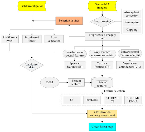
Figure 2.
Technical flowchart of discriminating urban forest types in our study. The step in the dashed-line rectangle represents the four support vector machine (SVM) classification models constructed with four different sets of features. SF refers to the spectral features; DEM refers to the digital elevation model, selected from terrain features; TF refers to the textural features; and VA refers to the vegetation abundances.
3.1. Linear Spectral Mixture Analysis
Due to rapid urban expansion and human activity, urban forests are increasingly fragmented and vegetated areas tend to be mixed pixels on satellite images. To address the mixed-pixel issue, linear spectral mixture analysis (LSMA), which treats the pixel spectrum as a linear combination of the endmember spectrums of the objects [53], can be used to extract vegetation endmembers and vegetation abundances (i.e., the proportion of vegetation to the area of a pixel), and to acquire more reliable training samples.
Three steps were required to perform LSMA on Sentinel-2A data. Firstly, a minimum noise fractionation (MNF) transformation, which is superior to principal component analysis (PCA) [54], was conducted to separate the band noise and minimize the intra-band correlations. In our study, the first six MNF components contained 80.94% of the original spectral variability and were, therefore, used for Cartesian coordinate system establishment and endmember selection in the second step. Vegetation endmembers usually lie at the vertices of the feature space constructed by combining any pair of the six MNF components. However, due to the similarity of spectral features between different forest types [55], such selection is not sufficient to get reliable vegetation endmembers. In the last step, these pre-selected endmembers were imported into ENVI’s interactive n-D Visualizer tool to generate pure pixels for spectral unmixing.
Fully constrained least squares (FCLS) is an LSMA method for endmember abundance calculation, which can simultaneously satisfy non-negativity (each abundance ranging between 0 and 1) and sum-to-unity (the sum of abundances for each pixel is 1) [53,56].
where R(λi) is the reflectance of the i pixel in the λ band, f(ki) is the proportion of the k endmember in the i pixel, C(kλ) is the reflectance of the k endmember in the λ band, m is the number of bands, and ε(λi) is the error value.
The root-mean-square error (RMSE) was used to assess the accuracy of FCLS in this study, which is given by
where m and ε(λi) have the same meanings as in Equations (1) and (2).
Three vegetation endmembers (broadleaved forest, coniferous forest, and low vegetation) were identified by trial and error, and their abundances were estimated through an FCLS spectral unmixing plugin of ENVI. For detailed results and analysis, see Section 4.1.
3.2. Selection of Features for Classification
For image classification, we preliminarily considered 126 features in total, ranging from spectral features and vegetation abundances to topographic features and textural features (Table 1). In addition to each spectral band, spectral features also included 30 spectral indices such as normalized difference vegetation index (NDVI) and normalized difference water index (NDWI). The features and their indicators are listed in Table 1. The abundances of the three vegetation endmembers (B1–B3 in Table 1) were coniferous forests, broadleaved forests, and low vegetation, which were obtained by the LSMA method (Section 4.1). Terrain features included a digital elevation model (DEM), and a DEM-derived slope and aspect. The textural features included eight types of textures such as mean, variance, and homogeneity, and were calculated using the gray-level co-occurrence matrix (GLCM) in ENVI. A total of 80 textural features in 10 bands (shown in Table 1, from D1–D80) were finally obtained.

Table 1.
Potential features for classification and their indicators.
However, in order to reduce data dimension and improve computational efficiency, the features should be selected prior to classification. As it can rank features in order of importance (a higher value implies a more important feature), random forest (RF) is often used for selecting essential features from a large number of features [58]. The number of decision trees in a random forest (mtree) and the number of features per node (ntry) are two key parameters in RF [59], and how they are combined impacts classification accuracy. Classification accuracy usually increases with the increase of mtree, and an optimal ntry is among , , and , where p is the number of features. This study set several different combinations of parameters and explored the effects of different parameter combinations on the feature importance. By constraining the range of mtree (100, 300, 500, 1000, 1500) and the range of ntry (5, 11, 22), random forest returned the importance of the 126 features for 15 different parameter combinations (Figure 3). Although the importance of each feature changed with parameter combination, their relative ranking almost always remained the same.
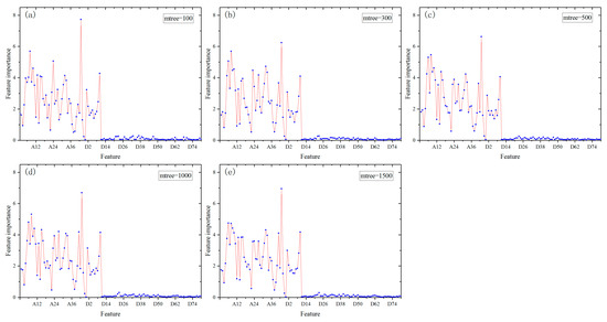
Figure 3.
Feature importance. A total of 15 parameter combinations were tested and only five (ntry = 11) are shown in the graph for illustration.
All the features were sorted in order of feature importance, and only those whose importance values were higher than 0.5 were selected to guarantee that each band had textural features to participate in the classification—because textural features proved important for land-cover classification in previous studies [60,61]. The chosen features used for classification are shown in Table 2. They were 54 in total, consisting of 40 spectral features, three vegetation abundance features, one terrain feature (i.e., DEM), and 10 textural features.
Table 2.
Features selected for image classification.
3.3. Support Vector Machine Classifier
The support vector machine (SVM) is a machine learning algorithm based on statistical learning theories. By constructing a classifying hyperplane, it can effectively solve the problems of limited, non-linear, and high-dimensional training samples [62]. If the samples are linearly separable, a linear discriminant function is established by constructing the classification surface to ensure the maximum distance between the samples. If the samples are linearly inseparable, the SVM projects the training samples to a high-dimensional space and finds the optimal classifying hyperplane [63].
In our study, we constructed four different SVM classification models differing in the feature used: Model 1 with spectral features (SF) (M1: SF); Model 2 with SF and digital elevation model (DEM) (M2: SF + DEM); Model 3 with SF, DEM, and textural features (TF) (M3: SF + DEM + TF); and Model 4 with SF, DEM, TF, and vegetation abundances (VA) (M4: SF + DEM + TF + VA). These four SVM classification models were tested to identify the best one for mapping and discriminating urban forest types of the study area. Classifications were implemented using an ENVI add-in known as EnMAP-box, which allows SVM and RF classifications [64]. The kernel function of the SVM classifications was Radial Basis Function (RBF), and the optimal penalty parameter (C) and the nuclear parameter (g) were determined by the grid search method [65]. Model accuracy was used to assess which parameter combination was best when constructing the SVM model with the training samples.
4. Results and Discussion
4.1. LSMA Result and Analysis
After MNF and endmember selection, three vegetation endmembers were identified, including broadleaved forest, coniferous forest, and low vegetation (Figure 4). Despite typical spectral signature vegetation with peaks and troughs located at quite similar wavelengths, they showed contrasting reflectance values in the same spectral range (e.g., 800–900 nm). In the visible part of the electromagnetic spectrum, low vegetation had higher reflectance than the other two types. This is because broadleaved forests can effectively use the red light and blue–violet light more efficiently than coniferous forests and low vegetation in photosynthesis [66]. However, highest reflectance was observed for low vegetation, and it was lowest for coniferous forest in the NIR–SWIR (near infrared-shortwave infrared) region, especially in the “vegetation red-edge” band (700–800 nm). This is likely to be explained by the complex canopy structures of low vegetation and broadleaved forests. Light cannot transmit them easily, resulting in increased reflections on the canopy surface. As for coniferous forests, their needle leaves are more prone to transmission and, thus, lower reflectance.
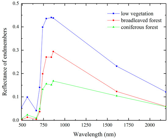
Figure 4.
Spectra of three vegetation endmembers.
Through the FCLS-based LSMA, three vegetation abundance maps were produced (Figure 5). All vegetation abundance values ranged from 0 to 1—a brighter pixel had a higher vegetation abundance value and vice versa. The RMSE of the FCLS was 0.019, indicating that our LSMA result is reliable [67].
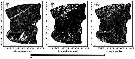
Figure 5.
Vegetation abundance maps: (a) coniferous forest; (b) broadleaved forest; (c) low vegetation.
As explained in Section 3.1, an abundance value refers to the ratio of the area of an urban forest type to the total area of a given pixel. Through the LSMA, the abundance of each forest type in every pixel can be derived. Given the spatial resolution of the image used (10 m × 10 m, i.e., the ground area of a pixel was 100 m2), the areas of different urban forest types in the study area were straightforwardly calculated (Table 3 and Figure 5). Results show that coniferous forests covered a maximal area of 15.28 km2 (accounting for 14.09% of the study area) and were mostly distributed on the hills of Yunlong, Zhushan, Zifang, and Jiuli (Figure 1d). They were dominated by Platycladus orientalis, mostly grown from local forestation projects between the 1950s and 1960s. Low vegetation (13.96 km2) was primarily distributed in parks and idle construction land, while broadleaved forests (4.21 km2) were mostly found in parks, rural settlements, and less hilly areas.
Table 3.
Areas of urban forest types in the study area.
4.2. Interpretation of Feature Importance
In this study, to determine a proper number of features used for urban forest discrimination, we first built a dataset of 126 candidate features and selected only 54 from them using the random forest. They covered a variety of spectral features (e.g., vegetation index and soil index), topographic features, and vegetation component abundances (Table 2). Among the features selected, spectral features like N_NIR, VRE2, and VRE3 bands (see their definitions in the note below Table 1) were highly ranked in the parameter combinations, suggesting their important roles in discrimination. This is not unexpected as these bands serve the vegetation monitoring purpose of the Sentinel-2A sensor, one of its major applications [44]. As reflectance at these bands is related to vegetation cellular structure [57] and varies with vegetation type, it is useful to use these bands to discriminate urban forest types [68]. We discuss textural features in Section 4.3.
4.3. SVM Classification Results and Accuracy Assessment
By means of the grid search method, the optimal values of parameters C and g for the four classification models were determined as (125, 0.04), (25, 0.2), (125, 0.4), and (625, 0.04), with model accuracies all being over 97%. Then, we performed the classifications and produced four different land-cover maps (Figure 6). Accuracy assessment based on the validation data acquired from our fieldwork showed that the highest accuracy and Kappa coefficient were achieved by M4 (89.86% and 0.83) and the lowest by M1 (86.96% and 0.79) (Table 4). Overall classification accuracy was improved by 1.45% when adding DEM to M1, and was further improved when textural features and vegetation abundances were added one by one. This suggests that classification accuracy tends to increase with the number of input features, which agrees with the study of Raczko and Zagajewski (2017) [69]. Reasons for the improvements vary. In the case of topography, it helps to improve classification accuracy because the impact of topography on vegetation growth is considered [70,71,72]. Textural features often prove useful in vegetation classification because vegetation texture varies with age, species, and many other factors [60,61]. Although only a few textural features were relatively highly ranked in terms feature importance, they might contribute to the improvement in classification accuracy. Vegetation abundances were shown to have a positive effect on classification, which is in agreement with the finding of Adams (1995) [39].
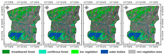
Figure 6.
Land-cover maps produced from the four SVM classification models: (a) M1 (SF); (b) M2 (SF + DEM); (c) M3 (SF + DEM + TF); (d) M4 (SF + DEM + TF + VA).
Table 4.
Accuracy assessment of the four support vector machine (SVM) classification models using the validation data acquired from fieldwork.
As M4 produced the best classification result, we here present its confusion matrix for a detailed analysis (Table 5). Both the highest user accuracy and producer accuracy were observed for the coniferous forest type. This is likely attributed to the fact that coniferous forests in the study area consisted mostly of Platycladus orientalis (L.) Franco, and these trees tend to grow in large numbers.
Table 5.
Confusion matrix of M4 (SF + DEM + TF + VA). Each row designates the classification result, and each column designates the field-based validation data.
The classification model (M4) resulting in the best accuracy (overall accuracy 89.86% and Kappa 0.83) was not employed in previous studies but it is still interesting to compare it with other urban vegetation classification studies. For example, De Colstoun et al. (2003) [73] mapped vegetation types in the Pennsylvania national forest park using a decision tree (C5.0) and multi-temporal Landsat data with an overall accuracy of 82.05% and a Kappa coefficient of 0.80. Liu and Yang (2013) [74] tested the multiple endmember spectral mixture analysis (MESMA) technique for urban vegetation classification with a maximal classification accuracy of 80.55%. Based on the SVM classifier, Poursanidis et al. (2015) [75] extracted urban land cover in the Greek city of Rafina by combining textural and spectral information, resulting in a highest classification accuracy of 89.23%. Compared with these studies, our method is more capable of discriminating different urban forest types.
4.4. Comparison of Different Classifier Results
In order to evaluate the differences between SVM and other machine learning classifiers for urban vegetation information extraction, and whether vegetation abundances can enhance urban vegetation discrimination similarly, three machine learning algorithms, i.e., RF (random forest), ANN (artificial neural network), and QUEST (quick unbiased efficient statistical tree), were used to discriminate urban forest types before and after adding vegetation abundances. The classification based on the SVM classification without vegetation abundance (i.e., M3, with 51 features) was labeled as SVM, and the SVM classification with vegetation abundances (i.e., M4, with 54 features) was labeled as SVM + VA. Similarly, we also named the RF-, ANN-, and QUEST-based classifications with and without vegetation abundances (Table 6).
Table 6.
Accuracy assessment of classifications comparing different machine learning classifiers.
As such, there were eight different classification models. These classifications were performed using the same training samples and assessed using validation data as the four SVM classifications in Table 4. For both RF classifications, their optimal mtry and ntry values were 1000 and 22 based on the result of out-of-bag error (OOB) test (see its definition in Li et al. (2017) [76]). The QUEST is a type of decision tree classifier and has a faster calculation and higher accuracy than other types [77]. Classification maps are presented in Figure 7 and the number of features, overall accuracy, and kappa coefficient for each classification model are shown in Table 6.
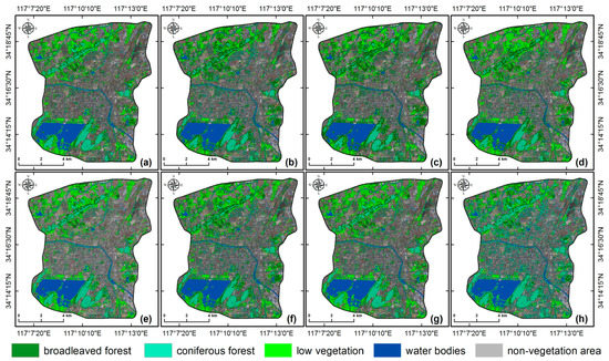
Figure 7.
Land-cover maps produced by eight different classification models: (a) SVM; (b) RF; (c) ANN; (d) QUEST; (e) SVM + VA; (f) RF + VA; (g) ANN + VA; and (h) QUEST + VA.
Among the eight classification models, the SVM + VA model obtained the highest accuracy (89.86%) and Kappa coefficient (0.83). In terms of classifier, SVM produced the best classification results, which agrees well with previous studies [8,36]. It has two evident advantages. Firstly, it can find an optimal hyperplane with the highest classification boundary in the n-dimensional feature space. This prevents the classifier from falling into local minima [63], which is the case for ANN. Secondly, SVM can minimize unseen errors in training samples [78] and, thus, a higher classification accuracy [79].
For each classifier, adding vegetation abundances in classification resulted in increased accuracy. This is particularly remarkable for the RF, ANN, and QUEST classifiers. Their classification accuracies were approximately 82% and the Kappa coefficients were less than 0.72, which rose to above 85% and 0.75, respectively. Classification accuracy of the SVM was also improved by including vegetation abundances, although such improvement was not that prominent. Additionally, our results suggest that ANN and RF could achieve similar classification accuracies, which was also confirmed by previous studies [80]. In our case, classification accuracies of ANN and RF were 82.14% and 81.29% before vegetation abundances were added, and increased by 2.86% and 2.92% for ANN and RF, respectively, after vegetation abundances were included.
In addition, if we examine the SVM- and RF-based classification maps closely (Figure 8), we can find that adding vegetation abundances resulted in more homogeneous classification maps. This is because it could effectively reduce the salt-and-pepper effect that usually occurs in pixel-based classification.
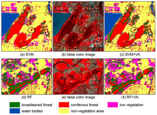
Figure 8.
Close examination of the SVM- and RF-based classification maps.
5. Conclusions
This study aimed at mapping and discriminating urban forest using single Sentinel-2A imagery and machine learning algorithms, such as SVM, ANN, RF, and QUEST. Input features were selected based on the feature importance of RF and included vegetation abundances obtained from linear spectral mixture analysis. From the results, we conclude the following:
- Three urban forest endmembers can be successfully identified from Sentinel-2A image data, and the LSMA method allows accurate mapping of their abundances with a low mean RMSE of 0.019.
- Classification accuracy of SVM classification tends to increase when spectral, topographic, and textural features and vegetation abundances are added one by one.
- The SVM classifier outperforms the other three machine learning algorithms based on the same classification samples and field-based validation data.
- Vegetation abundances help improve classification accuracy regardless of classifier.
Our study provides a basis for urban biomass estimation and has practical implications for forest management. It also demonstrates the capability of 10-m Sentinel-2A image data to discriminate vegetation types in a complex urban context. However, an avenue for future research would be to use different sources of remote-sensing data, such as Sentinel-1 SAR (Synthetic Aperture Radar) imagery. This might enable full use of the textural features of vegetation surfaces.
Author Contributions
X.Z. and L.L. conducted and designed the research plan and discussed it with L.C. who supervised and finalized the study. X.Z., Y.L., and Y.C. contributed to the design and conduction of fieldwork. Y.Z. and T.Z. were responsible for remote-sensing data collection and preprocessing. X.Z., L.L., and L.C. completed data analysis and the interpretation of results. X.Z. and L.L. wrote the manuscript, and all authors contributed to the revision and editing of the manuscript.
Funding
This research was supported by the Fundamental Research Funds for the Central Universities (Grant No.: 2018ZDPY07).
Acknowledgments
We would like to acknowledge the European Space Agency (ESA) for freely providing Sentinel-2A data required for the research, as well as the reviewers’ constructive comments and suggestions for the improvement of our study.
Conflicts of Interest
The authors declare no conflicts of interest.
Appendix A
Table A1.
Fieldwork sites for acquiring validation data for classification accuracy assessment.
Table A1.
Fieldwork sites for acquiring validation data for classification accuracy assessment.
| Number | X-coordinate | Y-coordinate | UF Types | Number | X-coordinate | Y-coordinate | UF Types |
|---|---|---|---|---|---|---|---|
| 1 | 514405 | 3787635 | BF | 2 | 514945 | 3787685 | BF |
| 3 | 515975 | 3787725 | CF | 4 | 516875 | 3787885 | CF |
| 5 | 515035 | 3787905 | CF | 6 | 517725 | 3787995 | BF |
| 7 | 517205 | 3788075 | CF | 8 | 517015 | 3788245 | CF |
| 9 | 515405 | 3788525 | CF | 10 | 517635 | 3788785 | CF |
| 11 | 516645 | 3788865 | BF | 12 | 517005 | 3789155 | BF |
| 13 | 518705 | 3789215 | LW | 14 | 518115 | 3789545 | LW |
| 15 | 516015 | 3790555 | BF | 16 | 519985 | 3793155 | BF |
| 17 | 512425 | 3793635 | LW | 18 | 512205 | 3794045 | CF |
| 19 | 512965 | 3794215 | CF | 20 | 513865 | 3794485 | CF |
| 21 | 513795 | 3794735 | CF | 22 | 514205 | 3795255 | BF |
| 23 | 516095 | 3796225 | CF | 24 | 516995 | 3796385 | BF |
| 25 | 513875 | 3797275 | LW | 26 | 517555 | 3797965 | LW |
| 27 | 520075 | 3786135 | LW | 28 | 517635 | 3786305 | CF |
| 29 | 520305 | 3786325 | BF | 30 | 519035 | 3786365 | LW |
| 31 | 520165 | 3786525 | BF | 32 | 517805 | 3786555 | CF |
| 33 | 518205 | 3786605 | BF | 34 | 513585 | 3786715 | BF |
| 35 | 518335 | 3786835 | CF | 36 | 518865 | 3786925 | BF |
| 37 | 514075 | 3787025 | LW | 38 | 517615 | 3787125 | BF |
| 39 | 513865 | 3787145 | BF | 40 | 513345 | 3787245 | LW |
| 41 | 515405 | 3787255 | BF | 42 | 516045 | 3787335 | CF |
| 43 | 514065 | 3787385 | BF | 44 | 514955 | 3787415 | BF |
| 45 | 515565 | 3787415 | CF | 46 | 513655 | 3787435 | BF |
| 47 | 517625 | 3787435 | BF | 48 | 519545 | 3787475 | CF |
| 49 | 518785 | 3787665 | BF | 50 | 515125 | 3787725 | CF |
| 51 | 513885 | 3787875 | BF | 52 | 515845 | 3787955 | CF |
| 53 | 512015 | 3787995 | BF | 54 | 512405 | 3788085 | CF |
| 55 | 517485 | 3788175 | BF | 56 | 515125 | 3788215 | BF |
| 57 | 513085 | 3788225 | BF | 58 | 515685 | 3788235 | CF |
| 59 | 511625 | 3788245 | BF | 60 | 512965 | 3788445 | BF |
| 61 | 511345 | 3788455 | LW | 62 | 517225 | 3788465 | CF |
| 63 | 517855 | 3788515 | BF | 64 | 517475 | 3788785 | LW |
| 65 | 511455 | 3788855 | BF | 66 | 516075 | 3788855 | BF |
| 67 | 515635 | 3788905 | BF | 68 | 516885 | 3789325 | BF |
| 69 | 511795 | 3789355 | LW | 70 | 515995 | 3789425 | BF |
| 71 | 520285 | 3789435 | BF | 72 | 519905 | 3789465 | BF |
| 73 | 515105 | 3789505 | LW | 74 | 520135 | 3789585 | BF |
| 75 | 513045 | 3789645 | CF | 76 | 512465 | 3789665 | BF |
| 77 | 516545 | 3789855 | BF | 78 | 519755 | 3789925 | BF |
| 79 | 519565 | 3790205 | BF | 80 | 516205 | 3790305 | BF |
| 81 | 512425 | 3791195 | BF | 82 | 514155 | 3791505 | BF |
| 83 | 519625 | 3792175 | CF | 84 | 518885 | 3792185 | CF |
| 85 | 520435 | 3792825 | BF | 86 | 512715 | 3792845 | BF |
| 87 | 519695 | 3793135 | BF | 88 | 513785 | 3793485 | LW |
| 89 | 512215 | 3793785 | LW | 90 | 512485 | 3793895 | BF |
| 91 | 512785 | 3793895 | CF | 92 | 513755 | 3794005 | BF |
| 93 | 511945 | 3794035 | BF | 94 | 517275 | 3794065 | BF |
| 95 | 512845 | 3794365 | LW | 96 | 515735 | 3794465 | BF |
| 97 | 513165 | 3794515 | LW | 98 | 512305 | 3794715 | BF |
| 99 | 514085 | 3794855 | CF | 100 | 512285 | 3794885 | LW |
| 101 | 512145 | 3795265 | BF | 102 | 513005 | 3795325 | BF |
| 103 | 515255 | 3795355 | BF | 104 | 511355 | 3795485 | BF |
| 105 | 515665 | 3795515 | BF | 106 | 515795 | 3795765 | CF |
| 107 | 514905 | 3795785 | BF | 108 | 512805 | 3795905 | BF |
| 109 | 513245 | 3795935 | BF | 110 | 514425 | 3795995 | LW |
| 111 | 515555 | 3795995 | CF | 112 | 516595 | 3796145 | CF |
| 113 | 511215 | 3796195 | BF | 114 | 515395 | 3796245 | LW |
| 115 | 514825 | 3796345 | BF | 116 | 516575 | 3796575 | BF |
| 117 | 511485 | 3796605 | BF | 118 | 517035 | 3796625 | BF |
| 119 | 512375 | 3796685 | CF | 120 | 515295 | 3796725 | LW |
| 121 | 516355 | 3796725 | LW | 122 | 517545 | 3796755 | LW |
| 123 | 517805 | 3796845 | BF | 124 | 518535 | 3796855 | LW |
| 125 | 517225 | 3796985 | LW | 126 | 518705 | 3797015 | CF |
| 127 | 512025 | 3797065 | BF | 128 | 514945 | 3797165 | LW |
| 129 | 513195 | 3797255 | LW | 130 | 513165 | 3797415 | BF |
| 131 | 517765 | 3797495 | LW | 132 | 518505 | 3797515 | LW |
| 133 | 515755 | 3797585 | CF | 134 | 515165 | 3797825 | LW |
| 135 | 516845 | 3797865 | BF | 136 | 518795 | 3797975 | LW |
| 137 | 519175 | 3798005 | CF | 138 | 515655 | 3798105 | LW |
| 139 | 516385 | 3798135 | BF | 140 | 518965 | 3798255 | LW |
Note: UF refers to urban forest, BF refers to broadleaved forest, CF refers to coniferous forest, and LW refers to low vegetation.
Table A2.
Formulas used for calculating spectral indices [55].
Table A2.
Formulas used for calculating spectral indices [55].
| Spectral Indices | Formula |
|---|---|
| Green index (GI) | |
| Green normalized different vegetation index (gNDVI) | |
| Normalized difference vegetation index (NDVI) | |
| Ratio vegetation index (RVI) | |
| Difference vegetation index (DVI) | |
| Enhanced vegetation index 2 (EVI2) | |
| Chlorophyll green index (Chlogreen) | |
| Normalized difference vegetation index (NDVIre1) | |
| Normalized difference vegetation index (NDVIre1n) | |
| Simple ratio 1 (SR1) | |
| Simple ratio 2 (SR2) | |
| Simple ratio 3 (SR3) | |
| Simple ratio 4 (SR4) | |
| Simple ratio 5 (SR5) | |
| Simple ratio 6 (SR6) | |
| Simple ratio 7 (SR7) | |
| Normalized difference water index (NDWI) | |
| Normalized difference water index 1 (NDWI1) | |
| Normalized difference water index 2 (NDWI2) | |
| Normalized humidity index (NHI) | |
| Normalized difference infrared index (NDII) | |
| Modified normalized difference water index (MNDWI) | |
| Normalized difference build-up index (NDBI) | |
| Build-up area index (BAI) | |
| Enhanced index-based built-up index (EIBI) | |
| Soil-adjusted vegetation index (SAVI) | |
| Modified soil-adjusted vegetation index 2 (MSAVI2) | |
| Optimized soil-adjusted vegetation index (OSAVI) | |
| Bare soil index (BSI) | |
| Normalized difference bareness and built-up index (NDBBI) |
Note: VRE1–VRE3 represent the three vegetation red-edge bands; N_NIR represents the narrow near-infrared bands.
References
- Dwivedi, P.; Rathore, C.S.; Dubey, Y. Ecological benefits of urban forestry: The case of Kerwa Forest Area (KFA), Bhopal, India. Appl. Geogr. 2009, 29, 194–200. [Google Scholar] [CrossRef]
- Young, R.F. Managing municipal green space for ecosystem services. Urban For. Urban Green. 2010, 9, 313–321. [Google Scholar] [CrossRef]
- Oliveira, S.; Andrade, H.; Vaz, T. The cooling effect of green spaces as a contribution to the mitigation of urban heat: A case study in Lisbon. Build. Environ. 2011, 46, 2186–2194. [Google Scholar] [CrossRef]
- Park, J.; Kim, J.-H.; Lee, D.K.; Park, C.Y.; Jeong, S.G. The influence of small green space type and structure at the street level on urban heat island mitigation. Urban For. Urban Green. 2017, 21, 203–212. [Google Scholar] [CrossRef]
- Inkiläinen, E.N.M.; McHale, M.R.; Blank, G.B.; James, A.L.; Nikinmaa, E. The role of the residential urban forest in regulating throughfall: A case study in Raleigh, North Carolina, USA. Landsc. Urban Plan. 2013, 119, 91–103. [Google Scholar] [CrossRef]
- Kirnbauer, M.C.; Baetz, B.W.; Kenney, W.A. Estimating the stormwater attenuation benefits derived from planting four monoculture species of deciduous trees on vacant and underutilized urban land parcels. Urban For. Urban Green. 2013, 12, 401–407. [Google Scholar] [CrossRef]
- Jensen, R.R.; Hardin, P.J.; Hardin, A.J. Classification of urban tree species using hyperspectral imagery. Geocarto Int. 2012, 27, 443–458. [Google Scholar] [CrossRef]
- Dalponte, M.; Bruzzone, L.; Gianelle, D. Tree species classification in the Southern Alps based on the fusion of very high geometrical resolution multispectral/hyperspectral images and LiDAR data. Remote. Sens. Environ. 2012, 123, 258–270. [Google Scholar] [CrossRef]
- He, C.; Convertino, M.; Feng, Z.; Zhang, S. Using LiDAR data to measure the 3D green biomass of Beijing urban forest in China. PLoS ONE 2013, 8, e75920. [Google Scholar] [CrossRef]
- Singh, K.K.; Chen, G.; McCarter, J.B.; Meentemeyer, R.K. Effects of LiDAR point density and landscape context on estimates of urban forest biomass. ISPRS J. Photogramm. Remote Sens. 2015, 101, 310–322. [Google Scholar] [CrossRef]
- Jorgensen, E. Urban forestry in the rearview mirror. Arboric. J. 1986, 10, 177–190. [Google Scholar] [CrossRef]
- McBride, J.; Jacobs, D. Urban forest development: A case study, Menlo Park, California. Urban Ecol. 1976, 2, 1–14. [Google Scholar] [CrossRef]
- Konijnendijk, C.C.; Ricard, R.M.; Kenney, A.; Randrup, T.B. Defining urban forestry—A comparative perspective of North America and Europe. Urban For. Urban Green. 2006, 4, 93–103. [Google Scholar] [CrossRef]
- Rowntree, R.A. Ecology of the urban forest—Introduction to part I. Urban Ecol. 1984, 8, 1–11. [Google Scholar] [CrossRef]
- Steenberg, J.W.N.; Duinker, P.N.; Charles, J.D. The neighbourhood approach to urban forest management: The case of Halifax, Canada. Landsc. Urban Plan. 2013, 117, 135–144. [Google Scholar] [CrossRef]
- Miller, R.W.; Hauer, R.J.; Werner, L.P. Urban Forestry: Planning and Managing Urban Greenspaces, 3rd ed.; Waveland Press Inc.: Long Grove, IL, USA, 2015; ISBN 9781478606376. [Google Scholar]
- Konijnendijk, C.C. A decade of urban forestry in Europe. For. Policy Econ. 2003, 5, 173–186. [Google Scholar] [CrossRef]
- Davies, H.J.; Doick, K.J.; Hudson, M.D.; Schreckenberg, K. Challenges for tree officers to enhance the provision of regulating ecosystem services from urban forests. Environ. Res. 2017, 156, 97–107. [Google Scholar] [CrossRef] [PubMed]
- Myeong, S.; Nowak, D.J.; Duggin, M.J. A temporal analysis of urban forest carbon storage using remote sensing. Remote. Sens. Environ. 2006, 101, 277–282. [Google Scholar] [CrossRef]
- Gunawardena, K.R.; Wells, M.J.; Kershaw, T. Utilising green and bluespace to mitigate urban heat island intensity. Sci. Total. Environ. 2017, 584–585, 1040–1055. [Google Scholar] [CrossRef]
- Nowak, D. Understanding the structure of urban forests. J. For. 1994, 92, 42–46. [Google Scholar]
- Ren, Z.; Zheng, H.; He, X.; Zhang, D.; Yu, X.; Shen, G. Spatial estimation of urban forest structures with Landsat TM data and field measurements. Urban For. Urban Green. 2015, 14, 336–344. [Google Scholar] [CrossRef]
- Trammell, T.L.E.; Carreiro, M.M. Vegetation composition and structure of woody plant communities along urban interstate corridors in Louisville, KY, U.S.A. Urban Ecosyst. 2011, 14, 501–524. [Google Scholar] [CrossRef]
- Fassnacht, F.E.; Latifi, H.; Stereńczak, K.; Modzelewska, A.; Lefsky, M.; Waser, L.T.; Straub, C.; Ghosh, A. Review of studies on tree species classification from remotely sensed data. Remote Sens. Environ. 2016, 186, 64–87. [Google Scholar] [CrossRef]
- Haapanen, R.; Ek, A.R.; Bauer, M.E.; Finley, A.O. Delineation of forest/nonforest land use classes using nearest neighbor methods. Remote Sens. Environ. 2004, 89, 265–271. [Google Scholar] [CrossRef]
- Martin, M.E.; Newman, S.D.; Aber, J.D.; Congalton, R.G. Determining forest species composition using high spectral resolution remote sensing data. Remote Sens. Environ. 1998, 65, 249–254. [Google Scholar] [CrossRef]
- Alonzo, M.; Roth, K.; Roberts, D. Identifying Santa Barbara’s urban tree species from AVIRIS imagery using canonical discriminant analysis. Remote Sens. Lett. 2013, 4, 513–521. [Google Scholar] [CrossRef]
- Pu, R.; Landry, S. A comparative analysis of high spatial resolution IKONOS and WorldView-2 imagery for mapping urban tree species. Remote Sens. Environ. 2012, 124, 516–533. [Google Scholar] [CrossRef]
- Pu, R.; Landry, S.; Zhang, J. Evaluation of atmospheric correction methods in identifying urban tree species with WorldView-2 imagery. IEEE J. Sel. Top. Appl. Earth Obs. Remote Sens. 2015, 8, 1886–1897. [Google Scholar] [CrossRef]
- Richter, R.; Reu, B.; Wirth, C.; Doktor, D.; Vohland, M. The use of airborne hyperspectral data for tree species classification in a species-rich Central European forest area. Int. J. Appl. Earth Obs. Geoinf. 2016, 52, 464–474. [Google Scholar] [CrossRef]
- Brovkina, O.; Cienciala, E.; Surový, P.; Janata, P. Unmanned aerial vehicles (UAV) for assessment of qualitative classification of Norway spruce in temperate forest stands. Geo-spatial Inf. Sci. 2018, 21, 12–20. [Google Scholar] [CrossRef]
- Reitberger, J.; Krzystek, P.; Stilla, U. Analysis of full waveform LiDAR data for the classification of deciduous and coniferous trees. Int. J. Remote Sens. 2008, 29, 1407–1431. [Google Scholar] [CrossRef]
- Linders, J. Comparison of three different methods to select feature for discriminating forest cover types using SAR imagery. Int. J. Remote Sens. 2000, 21, 2089–2099. [Google Scholar] [CrossRef]
- Alonzo, M.; Bookhagen, B.; McFadden, J.P.; Sun, A.; Roberts, D.A. Mapping urban forest leaf area index with airborne lidar using penetration metrics and allometry. Remote Sens. Environ. 2015, 162, 141–153. [Google Scholar] [CrossRef]
- Wang, K.; Wang, T.; Liu, X. A review: individual tree species classification using integrated airborne LiDAR and optical imagery with a focus on the urban environment. Forests 2018, 10, 1. [Google Scholar] [CrossRef]
- Ghosh, A.; Fassnacht, F.E.; Joshi, P.K.; Koch, B. A framework for mapping tree species combining hyperspectral and LiDAR data: Role of selected classifiers and sensor across three spatial scales. Int. J. Appl. Earth Obs. Geoinf. 2014, 26, 49–63. [Google Scholar] [CrossRef]
- Liu, L.; Coops, N.C.; Aven, N.W.; Pang, Y. Mapping urban tree species using integrated airborne hyperspectral and LiDAR remote sensing data. Remote Sens. Environ. 2017, 200, 170–182. [Google Scholar] [CrossRef]
- Tigges, J.; Lakes, T.; Hostert, P. Urban vegetation classification: Benefits of multitemporal Rapid Eye satellite data. Remote Sens. Environ. 2013, 136, 66–75. [Google Scholar] [CrossRef]
- Adams, J.B.; Sabol, D.E.; Kapos, V.; Almeida Filho, R.; Roberts, D.A.; Smith, M.O.; Gillespie, A.R. Classification of multispectral images based on fractions of endmembers: Application to land-cover change in the Brazilian Amazon. Remote. Sens. Environ. 1995, 52, 137–154. [Google Scholar] [CrossRef]
- Lu, D.; Weng, Q. Spectral mixture analysis of the urban landscape in Indianapolis with Landsat ETM+ imagery. Photogramm. Eng. Remote Sens. 2004, 70, 1053–1062. [Google Scholar] [CrossRef]
- Waske, B.; Benediktsson, J.A.; Árnason, K.; Sveinsson, J.R. Mapping of hyperspectral AVIRIS data using machine-learning algorithms. Can. J. Remote Sens. 2009, 35, S106–S116. [Google Scholar] [CrossRef]
- Dalponte, M.; Orka, H.O.; Gobakken, T.; Gianelle, D.; Naesset, E. Tree species classification in boreal forests with hyperspectral data. IEEE Trans. Geosci. Remote Sens. 2013, 51, 2632–2645. [Google Scholar] [CrossRef]
- Zhang, Y.; Chen, L.; Wang, Y.; Chen, L.; Yao, F.; Wu, P.; Wang, B.; Li, Y.; Zhou, T.; Zhang, T. Research on the contribution of urban land surface moisture to the alleviation effect of urban land surface heat based on Landsat 8 data. Remote Sens. 2015, 7, 10737–10762. [Google Scholar] [CrossRef]
- Drusch, M.; Del Bello, U.; Carlier, S.; Colin, O.; Fernandez, V.; Gascon, F.; Hoersch, B.; Isola, C.; Laberinti, P.; Martimort, P.; et al. Sentinel-2: ESA’s optical high-resolution mission for GMES operational services. Remote Sens. Environ. 2012, 120, 25–36. [Google Scholar] [CrossRef]
- MSI Instrument—Sentinel-2 MSI Technical Guide—Sentinel Online. Available online: https://sentinel.esa.int/web/sentinel/technical-guides/sentinel-2-msi/msi-instrument (accessed on 20 May 2019).
- Munyati, C. The potential for integrating Sentinel 2 MSI with SPOT 5 HRG and Landsat 8 OLI imagery for monitoring semi-arid savannah woody cover. Int. J. Remote Sens. 2017, 38, 4888–4913. [Google Scholar] [CrossRef]
- Forkuor, G.; Dimobe, K.; Serme, I.; Tondoh, J.E. Landsat-8 vs. Sentinel-2: examining the added value of sentinel-2’s red-edge bands to land-use and land-cover mapping in Burkina Faso. GIScience Remote Sens. 2018, 55, 331–354. [Google Scholar] [CrossRef]
- Fernández-Manso, A.; Fernández-Manso, O.; Quintano, C. SENTINEL-2A red-edge spectral indices suitability for discriminating burn severity. Int. J. Appl. Earth Obs. Geoinf. 2016, 50, 170–175. [Google Scholar] [CrossRef]
- Mura, M.; Bottalico, F.; Giannetti, F.; Bertani, R.; Giannini, R.; Mancini, M.; Orlandini, S.; Travaglini, D.; Chirici, G. Exploiting the capabilities of the Sentinel-2 multi spectral instrument for predicting growing stock volume in forest ecosystems. Int. J. Appl. Earth Obs. Geoinf. 2018, 66, 126–134. [Google Scholar] [CrossRef]
- Puliti, S.; Saarela, S.; Gobakken, T.; Ståhl, G.; Næsset, E. Combining UAV and Sentinel-2 auxiliary data for forest growing stock volume estimation through hierarchical model-based inference. Remote Sens. Environ. 2018, 204, 485–497. [Google Scholar] [CrossRef]
- Pesaresi, M.; Corbane, C.; Julea, A.; Florczyk, A.J.; Syrris, V.; Soille, P. Assessment of the added-value of Sentinel-2 for detecting built-up areas. Remote. Sens. 2016, 8, 299. [Google Scholar] [CrossRef]
- Main-Knorn, M.; Pflug, B.; Debaecker, V.; Louis, J. Calibration and validation plan for the L2a processor and products of the Sentinel-2 mission. ISPRS - Int. Arch. Photogramm. Remote Sens. Spat. Inf. Sci. 2015, XL-7/W3, 1249–1255. [Google Scholar] [CrossRef]
- Li, L.; Canters, F.; Solana, C.; Ma, W.; Chen, L.; Kervyn, M. Discriminating lava flows of different age within Nyamuragira’s volcanic field using spectral mixture analysis. Int. J. Appl. Earth Obs. Geoinf. 2015, 40, 1–10. [Google Scholar] [CrossRef]
- Zhang, C.; Xie, Z. Combining object-based texture measures with a neural network for vegetation mapping in the Everglades from hyperspectral imagery. Remote Sens. Environ. 2012, 124, 310–320. [Google Scholar] [CrossRef]
- Schmidt, K.S.; Skidmore, A.K. Spectral discrimination of vegetation types in a coastal wetland. Remote. Sens. Environ. 2003, 85, 92–108. [Google Scholar] [CrossRef]
- Zhang, Y.; Li, L.; Chen, L.; Liao, Z.; Wang, Y.; Wang, B.; Yang, X. A modified multi-source parallel model for estimating urban surface evapotranspiration based on ASTER thermal infrared data. Remote Sens. 2017, 9, 1029. [Google Scholar] [CrossRef]
- Njoku, E.G. Encyclopedia of Remote Sensing; Springer Science: New York, NY, USA, 2014; ISBN 9780387366982. [Google Scholar]
- Ma, L.; Fan, S. CURE-SMOTE algorithm and hybrid algorithm for feature selection and parameter optimization based on random forests. BMC Bioinform. 2017, 18, 169. [Google Scholar] [CrossRef]
- Cui, Y.; Li, L.; Chen, L.; Zhang, Y.; Cheng, L.; Zhou, X.; Yang, X. Land-use carbon emissions estimation for the Yangtze River Delta urban agglomeration using 1994–2016 landsat image data. Remote Sens. 2018, 10, 1334. [Google Scholar] [CrossRef]
- Immitzer, M.; Atzberger, C.; Koukal, T. Tree species classification with random forest using very high spatial resolution 8-band WorldView-2 satellite data. Remote. Sens. 2012, 4, 2661–2693. [Google Scholar] [CrossRef]
- Dian, Y.; Li, Z.; Pang, Y. Spectral and texture features combined for forest tree species classification with airborne hyperspectral imagery. J. Indian Soc. Remote Sens. 2015, 43, 101–107. [Google Scholar] [CrossRef]
- Nello, C.; John, S. An Introduction to Support Vector Machines and Other Kernel-Based Learning Methods; Cambridge University Press: Cambridge, UK, 2000. [Google Scholar]
- Cervantes, J.; Garcia-Lamont, F.; Rodriguez, L.; López, A.; Castilla, J.R.; Trueba, A. PSO-based method for SVM classification on skewed data sets. Neurocomputing 2017, 228, 187–197. [Google Scholar] [CrossRef]
- Van Der Linden, S.; Rabe, A.; Held, M.; Jakimow, B.; Leitão, P.J.; Okujeni, A.; Schwieder, M.; Suess, S.; Hostert, P. The EnMAP-Box—A toolbox and application programming interface for EnMAP data processing. Remote. Sens. 2015, 7, 11249–11266. [Google Scholar] [CrossRef]
- Bao, Y.; Hu, Z.; Xiong, T. A PSO and pattern search based memetic algorithm for SVMs parameters optimization. Neurocomputing 2013, 117, 98–106. [Google Scholar] [CrossRef]
- Yu, Q.; Wang, S.; Huang, K.; Zhou, L.; Chen, D. An anlysis of the spectrums between different canopy structures based on Hypersion hyperspectral data in a temperate forest of North China. Spectrosc. Spectr. Anal. 2015, 35, 1980–1985. [Google Scholar]
- Wu, C.; Murray, A.T. Estimating impervious surface distribution by spectral mixture analysis. Remote Sens. Environ. 2003, 84, 493–505. [Google Scholar] [CrossRef]
- Canetti, A.; Garrastazu, M.C.; De Mattos, P.P.; Braz, E.M.; Netto, S.P. Understanding multi-temporal urban forest cover using high resolution images. Urban For. Urban Green. 2018, 29, 106–112. [Google Scholar] [CrossRef]
- Raczko, E.; Zagajewski, B. Comparison of support vector machine, random forest and neural network classifiers for tree species classification on airborne hyperspectral APEX images. Eur. J. Remote Sens. 2017, 50, 144–154. [Google Scholar] [CrossRef]
- Fahsi, A.; Tsegaye, T.; Tadesse, W.; Coleman, T. Incorporation of digital elevation models with Landsat-TM data to improve land cover classification accuracy. For. Ecol. Manag. 2000, 128, 57–64. [Google Scholar] [CrossRef]
- Gislason, P.O.; Benediktsson, J.A.; Sveinsson, J.R. Random Forests for land cover classification. Pattern Recognit. Lett. 2006, 27, 294–300. [Google Scholar] [CrossRef]
- Gartzia, M.; Alados, C.L.; Pérez-Cabello, F.; Bueno, C.G. Improving the accuracy of vegetation classifications in mountainous areas. Mt. Res. Dev. 2013, 33, 63–74. [Google Scholar] [CrossRef]
- De Colstoun, E.C.B.; Story, M.H.; Thompson, C.; Commisso, K.; Smith, T.G.; Irons, J.R. National Park vegetation mapping using multitemporal Landsat 7 data and a decision tree classifier. Remote. Sens. Environ. 2003, 85, 316–327. [Google Scholar] [CrossRef]
- Liu, T.; Yang, X. Mapping vegetation in an urban area with stratified classification and multiple endmember spectral mixture analysis. Remote Sens. Environ. 2013, 133, 251–264. [Google Scholar] [CrossRef]
- Poursanidis, D.; Chrysoulakis, N.; Mitraka, Z. Landsat 8 vs. Landsat 5: A comparison based on urban and peri-urban land cover mapping. Int. J. Appl. Earth Obs. Geoinf. 2015, 35, 259–269. [Google Scholar] [CrossRef]
- Li, L.; Solana, C.; Canters, F.; Kervyn, M. Testing random forest classification for identifying lava flows and mapping age groups on a single Landsat 8 image. J. Volcanol. Geotherm. Res. 2017, 345, 109–124. [Google Scholar] [CrossRef]
- Hasan, R.C.; Ierodiaconou, D.; Monk, J. Evaluation of four supervised learning methods for benthic habitat mapping using backscatter from multi-beam sonar. Remote. Sens. 2012, 4, 3427–3443. [Google Scholar] [CrossRef]
- Mountrakis, G.; Im, J.; Ogole, C. Support vector machines in remote sensing: A review. ISPRS J. Photogramm. Remote Sens. 2011, 66, 247–259. [Google Scholar] [CrossRef]
- Petropoulos, G.P.; Kontoes, C.C.; Keramitsoglou, I. Land cover mapping with emphasis to burnt area delineation using co-orbital ALI and Landsat TM imagery. Int. J. Appl. Earth Obs. Geoinf. 2012, 18, 344–355. [Google Scholar] [CrossRef]
- Li, W.; Fu, H.; Yu, L.; Gong, P.; Feng, D.; Li, C.; Clinton, N. Stacked Autoencoder-based deep learning for remote-sensing image classification: a case study of African land-cover mapping. Int. J. Remote Sens. 2016, 37, 5632–5646. [Google Scholar] [CrossRef]
© 2019 by the authors. Licensee MDPI, Basel, Switzerland. This article is an open access article distributed under the terms and conditions of the Creative Commons Attribution (CC BY) license (http://creativecommons.org/licenses/by/4.0/).