Mapping Coarse Woody Debris with Random Forest Classification of Centimetric Aerial Imagery

Abstract

Coarse woody debris (CWD; large parts of dead trees) is a vital element of forest ecosystems, playing an important role in nutrient cycling, carbon storage, fire fuel, microhabitats, and overall forest structure. However, there is a lack of effective tools for identifying and mapping both standing (snags) and downed (logs) CWD in complex natural settings. We applied a random forest machine learning classifier to detect CWD in centimetric aerial imagery acquired over a 270-hectare study area in the boreal forest of Alberta, Canada. We used a geographic object-based image analysis (GEOBIA) approach in the classification with spectral, spatial, and LiDAR (light detection and ranging)-derived height predictor variables. We found CWD to be detected with great accuracy (93.4 ± 4.2% completeness and 94.5 ± 3.2% correctness) when training samples were located within the application area, and with very good accuracy (84.2 ± 5.2% completeness and 92.2 ± 3.2% correctness) when training samples were located outside the application area. The addition of LiDAR-derived variables did not increase the accuracy of CWD detection overall (<2%), but aided significantly (p < 0.001) in the distinction between logs and snags. Foresters and researchers interested in CWD can take advantage of these novel methods to produce accurate maps of logs and snags, which will contribute to the understanding and management of forest ecosystems.

1. Introduction

Woody debris—dead trees and branches—is a key element of forest ecosystems, providing nutrient cycling, carbon storage, microhabitats, and overall forest structure, and can feature prominently in studies of wildlife habitat [1], forest fuel load [2], bioenergy [3], and forest disturbances [4]. Coarse woody debris (CWD) can be distinguished from fine woody debris on the basis of length (at least 1 m) and diameter (at least 10 cm at the largest end) [5]. The two most common classes of CWD are snags and logs. If the CWD is standing with an inclination relative to vertical smaller than 45° then it can be classified as a snag. If it is positioned horizontally or is leaning with an inclination greater than 45° relative to vertical then it is classified as a log [5].

In the boreal forest of Alberta, Canada, extensive human disturbances, mostly side products of resource development such as roads, mineral exploration corridors, and well-sites, have been shown to increase predation rates on woodland caribou (Rangifer tarandus), especially by wolves (Canis lupus) [6]. This is one of the reasons why caribou populations in Alberta have declined significantly in the last two decades and consequently the species has been listed as threatened by the federal and provincial governments [7]. Within this context, CWD is especially important, since it is widely applied to linear-disturbance features to obstruct the movement of predators and humans, while creating valuable microsites for improved growth and protection of newly planted seedlings [8].

Traditional methods for detecting and measuring CWD rely on manual field operations—an activity that is labor intensive and difficult to scale. Therefore, a variety of studies have applied remote sensing solutions to detect CWD. For example, Inoue et al. [9] used nadir-looking air photos of ground sampling distance (GSD) around 1 cm obtained with an unmanned aerial vehicle (UAV) to visually detect logs under leaf-off conditions in a temperate deciduous forest, achieving about 85% completeness on CWD detection. The authors concluded that this kind of approach is promising for lowering costs of ground surveys, but the study area was small (200 × 300 m), focused only on logs, and involved identification through visual detection—a strategy that would be inappropriate over large areas.

Some studies have used satellite data to delineate CWD. For example, Baumann et al. [10] applied support vector machine classification on multi-temporal Landsat data to detect windthrown areas with good accuracy (about 95% completeness and 67% correctness). Similarly, Rüetschi et al. [11] detected windthrown areas through multi-temporal analysis of Sentinel-1 C-band datasets, obtaining reliable results (88% completeness and 85% correctness). However these approaches are generally only suitable for detecting large windthrow disturbances.

Light detection and ranging (LiDAR) has been used in many studies of forest structure, including some aimed at the detection of CWD. For example, Sumnall et al. [12] applied regression of LiDAR statistics on study plots, obtaining a strong relationship with snag volume (R² = 0.91) but weaker for log volume (R² = 0.51). Their strategy did not involve the explicit detection of CWD objects, but rather relied on implicit relationships between field measurements and LiDAR-derived metrics. It is unclear how well such relationships would extend beyond their study site in southern England.

There have been few studies presenting accurate methods for detecting individual CWD objects in forested environments. Polewski [13] detected logs in a forested area via multiple classification steps over a LiDAR point cloud (30 points/m²), obtaining good results (~80% completeness and correctness). Richardson and Moskal [14] detected logs in riparian areas via a rule-based geographical object image analysis (GEOBIA) workflow applied to LiDAR (8 points/m²) and four-band imagery (15 cm GSD), reporting a good relationship between measured and predicted CWD area (R² = 0.65). Stereńczak et al. [15] detected snags via maximum likelihood classification of LiDAR (6 points/m²) and four-band data (<50 cm GSD), achieving high-accuracy products (93.65% completeness and 99.95% correctness of testing points). Duan et al. [16] classified wind-thrown logs on visible band (RGB) UAV images (20 cm GSD) through random forest classification of image pixels. The authors then used a Hough-transform algorithm to delineate each log object, reporting good results (75.7% completeness and 92.5% correctness). A study by Panagiotidis et al. [17] also detected wind-thrown logs in a forest environment by processing UAV-obtained aerial images (3 cm GSD) via a series of edge-detection filters and then applying the Hough transform to delineate individual logs, with good results (84.6% completeness and 94.9% correctness).

None of the studies listed above has attempted to identify both logs and snags through a single classification method, none has used object-based classification in conjunction with area-based verification, and none has been applied to the boreal ecosystem. Additionally, except for Richardson and Moskal [14] and Stereńczak et al. [15], all previous studies used very small application areas and focused only on recently downed trees (wind-throws). Thus, additional studies are required aimed at larger, more complex study areas in a broad variety of settings.

The aim of this study was to develop and test a GEOBIA-based workflow for classifying logs and snags in the boreal forest using random-forest classification of multispectral and LiDAR data acquired from an aerial platform. In pursuing this work, we addressed two main objectives. First, we assessed the accuracy and transferability of our workflow by conducting validation exercises in both a calibration area, where the classifier was trained, and a separate verification area located in another portion of the study area. Second, we evaluated the need for supplementary LiDAR metrics in this classification task. Additional analyses were performed to gain insight into the number of predictor variables required to map CWD effectively with random forest, and the effect of training-dataset size on classification accuracy.

2. Materials and Methods

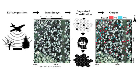
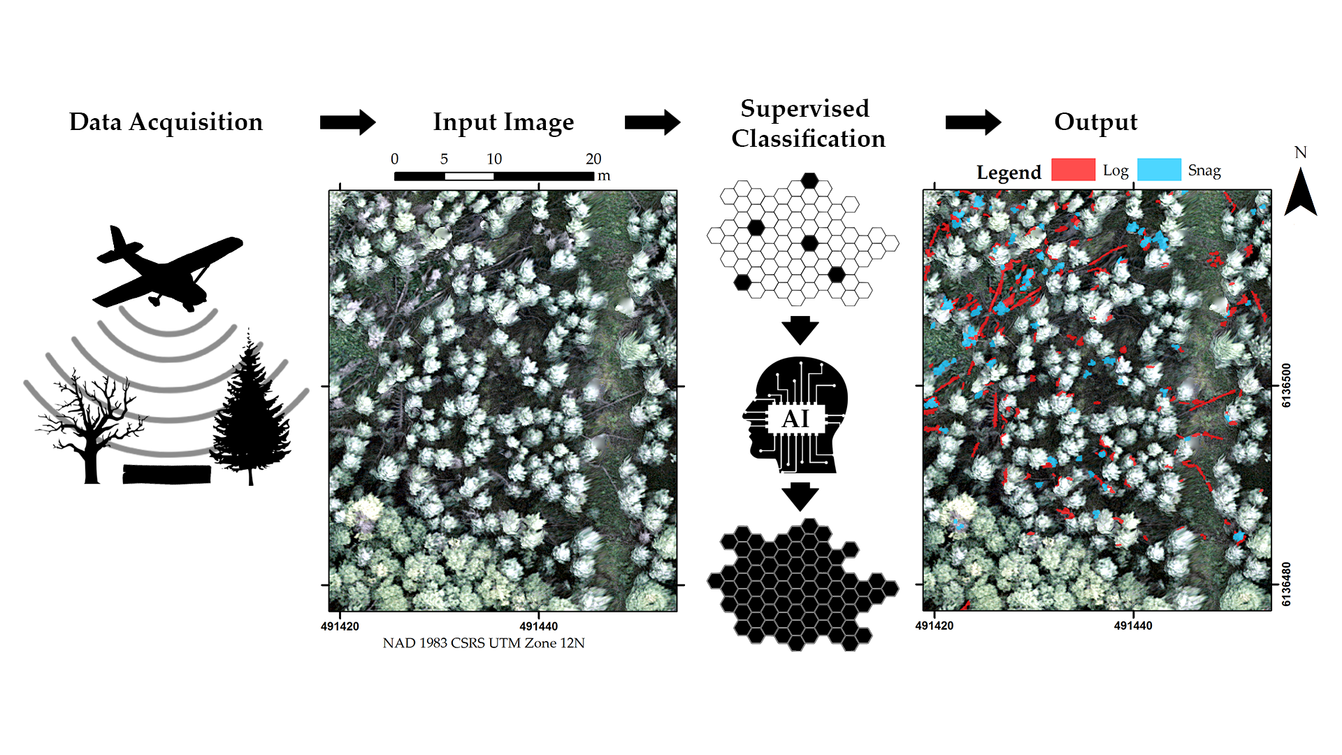
This paper presents a novel approach to CWD detection in centimetric (i.e., dimensioned in the order of centimeters) aerial imagery using a geographic object-based image analysis (GEOBIA) workflow, where the image-objects are classified by a random forest (RF) using spectral and LiDAR data as predictor variables. In this demonstration, we identify logs and snags in a boreal forest study site located in northern Alberta, Canada.

GEOBIA consists in partitioning images into a set of mutually exclusive and collectively exhaustive groups of connected pixels (a.k.a. image-objects) that are relatively homogeneous internally, and then analyzing such objects based on their spectral and spatial features [18]. Random forest is a machine-learning algorithm that creates (trains) an ensemble of classification trees, each with a distinct random selection of the input features, then classifies objects through a voting system for all created trees [19]. The approach has been previously demonstrated to be efficient in classifying log objects [16].

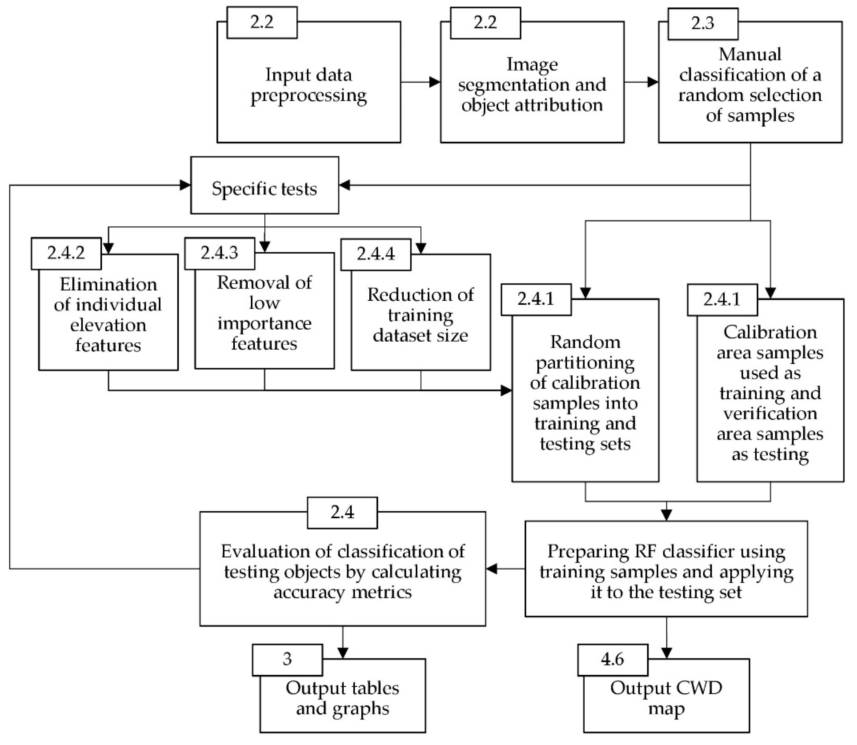
To assess accuracy, we conducted a number of experiments. The main one assessed the accuracy of our approach for classifying CWD in both the calibration (where the classifier was trained and tested) and the verification (a separate portion only used for testing) parts of the study area. A second set of experiments involved removing certain predictor variables from the training process and assessing their effect on accuracy. Finally, a training-dataset-size test was performed by gradually reducing the number of training samples and assessing the trade-offs in classification accuracy.

A graphical summary of our workflow and the tests performed in this study is shown in Figure 1; details are provided in the following subsections. Image segmentation and image-object attribution with spatial and spectral features were performed in eCognition (Version 9.4) [20]. All other procedures, including training random forest and assessing the accuracy of classifiers, were performed in R (Version 3.5.1) [21] using the “randomforest” package [22]. The source code in R and input files used to generate the results presented in this paper are provided as Supplementary material.

2.1. Study Area

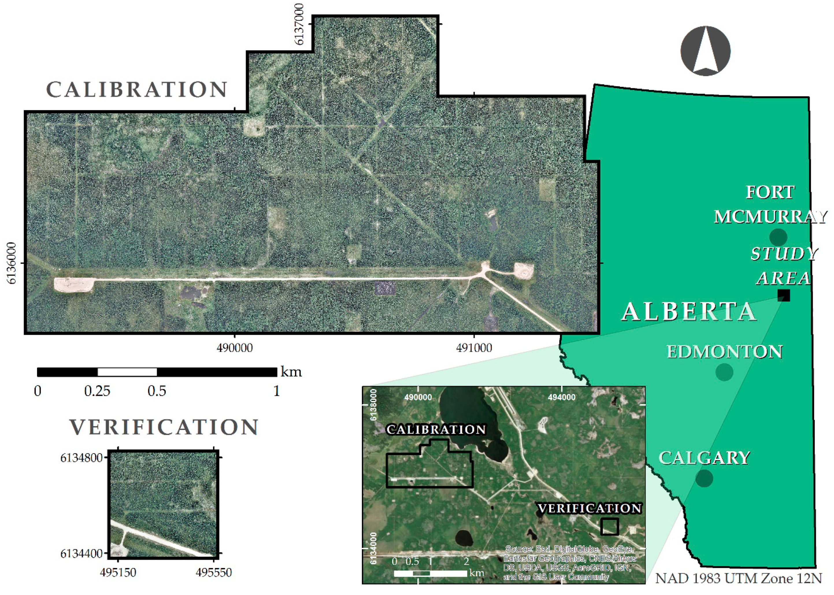
The study area (Figure 2) is located in the boreal forest natural region near Conklin, Alberta, in the central mixed-wood subregion [23]. The gently rolling terrain, which can be divided into uplands and wetlands, is mainly populated by jack pine (Pinus banksiana Lamb.), black spruce (Picea mariana (Mill.) B.S.P.), and trembling aspen (Populous tremuloides Michx.) trees [23]. The region contains a dense network of reclaimed and un-reclaimed seismic lines (petroleum exploration corridors 5–10 m wide) and well sites. CWD can be found dispersed in the undisturbed forest, as well as concentrated in piles on seismic lines. The study area was selected for being representative of its natural subregion, as well as containing a good variety of disturbances and restoration strategies on seismic lines. A 250-hectare calibration area was selected to develop and fine-tune the CWD classification method. A smaller 20-hectare verification area, about 4 km SE of the calibration area, was used to assess the accuracy of the classifier developed in the calibration area when applied “as is” to a similar area with no further training or tuning.

2.2. Image Acquisition and Pre-Processing

Remote sensing data for this project were obtained via a piloted aircraft (Cessna 210T) mission executed by OGL Engineering of Calgary on August 2 and 4, 2017. The aircraft was equipped with a LiDAR sensor (Leica ALS70, Leica Geosystems AG, Heerbrugg, Switzerland), an optical sensor (Leica RCD30, Leica Geosystems AG, Heerbrugg, Switzerland), a global navigation satellite system (GNSS, Rohde & Schwarz, Munich, Germany) unit, and an inertial measurement unit. The flight detail for this mission is provided in

Table 1. Flight specifications for airborne remote sensing mission. Projection uses the Canadian Spatial Reference System (CSRS) in Universal Transverse Mercator (UTM) coordinates.

Projection/Datum	NAD83 (CSRS) UTM Zone 12N, CGVD2013
Flying Height	850 m Above Ground Level
Flying speed	130 knots, 67 m/s
Overlap	80% forward and 60% side
Ground Resolution (RGB)	5.5 cm or less
Sensor calibration	Yes, Leica Geosystems

. Prior to the flight mission, 250 visible ground control points (GCPs, 60 cm squares with a bullseye marking) were deployed across the study area and their coordinates measured using a real-time kinematic GNSS (Trimble R8 – 8 mm horizontal and 15 mm vertical precision - Trimble, Sunnyvale, United States). Out of the 250 GCPs, 100 were used for georeferencing, and the remaining 150 were used for accuracy assessment. The X, Y, and Z accuracy (root-mean-square error) of the final products were 5, 10, and 11 cm, respectively.

The average raw LiDAR point density was ~40 pts/m². OGL Engineering (Orthoshop Geomatics Ltd.) Calgary performed noise removal from the raw points, then classified them into ground and non-ground points, using Bentley Microstation with Terrasolid software to accomplish this task. We then rasterized (25 cm pixel) the ground points into a digital terrain model (DTM) and the first-return points into a digital surface model (DSM) in ESRI (Environmental Systems Research Institute) ArcMAP (Version 10.6.1) [24]. Finally, a canopy height model (CHM) was obtained by subtracting the DTM from the DSM.

We used a structure-from-motion [25] workflow in Agisoft Photoscan (Version 1.2.4.2399) [26] to generate a photogrammetric point cloud and an orthomosaic from the raw photos (~2200). However, only the orthomosaic was used for this project. First, the photo quality was assessed using Agisoft Photoscan photo-quality assessment tool. All the photos were found to be above the minimum quality threshold. Then, the photos were aligned and a sparse point cloud was generated using the camera positions estimated by the onboard GPS. The camera position and orientation, and the X, Y, and Z locations of the sparse point cloud were further adjusted with the georeferenced GCPs. The sparse point cloud was next used to generate a dense point cloud and DSM. Finally an orthomosaic was generated at 5 cm GSD using the true DSM. A normalized difference vegetation index (NDVI) for the area of study was also generated from the Red and the Near-infrared (NIR) bands of the orthomosaic.

The LiDAR DSM and CHM, the orthorectified Red, Green, Blue, and NIR bands, and NDVI were stacked together and used as input image bands in Trimble eCognition (Version 9.4). Only the Red, Green, Blue, NIR, and NDVI bands were used for image segmentation (i.e., creation of image-objects), since the LiDAR layers had a less dense GSD (25 cm) and were too smooth to provide information about the edge of objects, while all the input bands were used to attribute the generated image-objects. After some initial testing to find a reasonable balance between under- and over-segmentation, the segmentation parameters were set to scale 10, shape 0.6, and compactness 0.4. The resulting image-objects and their attributes were used for further analysis.

2.3. Training the Classifier

A reference dataset in the calibration area was created by manually classifying 5000 randomly selected image-objects (hereafter called just “objects” for short). To account for the lower frequency in the orthomosaic of objects with a NDVI similar to that of CWD (<−0.1 in the NDVI image), a stratified random sample with two strata (with −0.1 separating “high” vs. “low” NDVI) was extracted. Out of the 5000 objects, 1000 came from the “high” NDVI stratum and 4000 and 1000 from the “low” NDVI objects. Similarly, a second randomly selected reference dataset was created in the verification area, with 300 “high”-NDVI objects and 1200 “low”-NDVI objects. Objects in these datasets were classified by an experienced human analyst. The analyst viewed the reference-object polygons and the spectral and height layers in a GIS environment, then labeled the 6500 calibration-verification objects with one of the classes in

Table 2. Name and description of each of the classes in the reference dataset. The five first classes were used for training and testing (Y) the random forest classifier, and the last two were not used for either training or testing but for discarding some of the randomly selected objects (N).

Name	Description	Train/Test
Log	Downed CWD. Horizontal or leaning with an angle ≥ 45°	Y
Snag	Standing CWD. Vertical or leaning with an angle < 45°	Y
Water	Puddles and ponds	Y
Dirt	Road, mud and exposed soil	Y
Other	Shrubs, moss, alive trees, shadowed areas	Y
Man-made	Ground control points, buildings, power lines	N
Unidentified	Unclassifiable object due to practical issues or limitations	N

.

The five object classes used for random forest classification were as follows: logs, snags, water, dirt, and other (Table 2). This class composition was deemed to be optimal for the present study after preliminary accuracy tests were performed with different combinations of training classes. Using just the classes of interest (log and snag plus “other”) decreased the number of false positives, but also increased the number of false negatives. By adding water and dirt as formal classes, which correspond to low-NDVI objects often confused with CWD, we obtained a better trade-off between false positives and false negatives.

Objects that the human analyst was unable to unambiguously identify were labeled as unidentified and discarded from the reference dataset. Common unidentified objects included miniscule features composed of few pixels, heavily shaded objects that are distinct from their surroundings but too dark to identify, and blurry objects positioned in areas where the ortho-mosaicking produced artifacts.

The reference dataset for the calibration area had 3710 objects, of which 364 were logs and 537 were snags. The remaining objects in the calibration area of the original 5000 were discarded for being unidentified and not beneficial for training. The reference dataset for the verification area had 1500 objects, of which 40 were logs, 51 were snags, and 192 were unidentified objects. More detail and descriptions about each class can be found in Appendix A.

The manually classified image-objects had spatial, spectral, and height attributes that were exported from eCognition for use as predictor variables in R. The spectral attributes for each band and height layer included the following: mean, standard deviation, difference from neighbors, band ratio, border contrast, mean inner border, mean outer border, minimum, maximum, and skewness. The spatial attributes included density, asymmetry, length by width, border length by length, shape index, compactness, polygon width, pixel area, border index, main line width, pixel length, rectangular fit, perimeter, roundness, elliptic fit, and curvature by length. Full attribute definitions can be found in the eCognition Reference Book [27].

Before running the random forest classification in the calibration area, a stratified-random selection of the reference dataset was performed. In each run, we used 80% of the reference objects for training and 20% for testing, while maintaining the original proportion of object classes. No training was performed in the verification area. Out of the 1500 reference objects in it, 1388 were used for testing, and the remaining 192 unidentified objects were discarded.

2.4. Classification Accuracy Analysis

Random forest classifiers, specific for each individual test (explained in the following subsections), were trained using their respective training datasets and then tested against reference data. In this manner, we created confusion matrices and derived two accuracy metrics: completeness and correctness. Completeness indicates the areal proportion (i.e., proportion by total area, not by number of objects) of all the target-class objects in the test data which were correctly assigned the target class. Correctness is the areal proportion of all objects in the target class that actually belong to this class in the reference data. These metrics are calculated as:

$$Completeness=\frac{TP}{TP+FN}=1-Omission$$

(1)

$$Correctness=\frac{TP}{TP+FP}=1-Comission$$

(2)

where TP is the total area of true positives: actual target class objects correctly classified as such; FN is the total area of false negatives: actual target class objects incorrectly classified with a different class; and FP total area of false positives: non-target objects incorrectly classified as the target class. In this study, we defined target classes at two hierarchical levels: (i) logs and snags at the lower level; and (ii) a “CWD union” class at the upper level, which represents all CWD objects together.

Since there can be variability in the results due to the training and testing selection, as well as in the way the RF algorithm constructs the classification trees, the accuracy metrics in this study were obtained by running 100 independent instances of random forests for each test (i.e., for each instance, an independent 80/20 training/testing stratified random split was drawn from the reference dataset of the calibration area). Results are reported as averages (arithmetic mean) and standard deviations.

2.4.1. General Accuracy and Transferability

In order to test the reliability of our workflow for CWD identification, we applied it first to the calibration area and then to the verification area. In the calibration area, a random selection of 80% of the reference samples were used to train the classifier. The remaining 20% were used for testing (i.e., for assessing the performance of the classifier). We repeated this process 100 times and averaged the results. In order to test the transferability of the classifier to a spatially segregated area, we performed a second test using the reference objects in the verification area. This test was also repeated 100 times (once per each classifier instance) and the results were averaged.

2.4.2. Value of LiDAR-Derived Height Variables

Two types of height data were tested in this study: a digital surface model (DSM) and a canopy height model (CHM), both derived from LiDAR. We tested their effect on RF classifier accuracy using four combinations of predictors: (i) all spectral and height attributes; (ii) all spectral data plus CHM data; (iii) all spectral data plus DSM data; and (iv) only spectral attributes. Each of these combinations were used in 100 RF runs, and their results were averaged. We used a series of pairwise difference-of-means t-tests to look for statistically significant differences on completeness and correctness accuracies in each of the three CWD classes: CWD union, logs, and snags. The null hypothesis was that there is no difference in the mean accuracy of any given CWD class between one combination of predictor variables and another. The significance level for these t-tests was 0.05.

2.4.3. Importance of Predictor Variables

The Random Forest R package provides a built-in “importance” function, which measures the impact of each predictor variable on classification error by calculating the difference between the error before and after randomizing each variable [22]. More important variables have a greater effect on classification accuracy, and therefore receive a higher importance score. For example, a variable with an importance score of 20 means that randomly permuting the values of that variable leads to a 20% decrease in accuracy. These values are discriminated for each of the output classes. The importance values of 100 RF for the two CWD classes (logs and snags) were averaged and then the predictor variables were ranked from most important to least important in terms of CWD detection accuracy. In order to test the effect of the number of predictor variables on CWD classification accuracy, the least-important variables were gradually removed one by one. We performed classification-accuracy tests for each iteration, based on 100 random forests, until no more variables could be removed.

2.4.4. Effect of Training-Sample Size

We tested the effect of training-sample size on classification accuracy by systematically reducing the number of training samples—from 2374 (64% of the calibration reference) down to 32—while maintaining a constant number of testing samples (592 samples, 16% of the reference). For each iteration the classification accuracy average and standard deviation of 100 RF runs was calculated, where every forest had samples selected through stratified-random sampling.

3. Results

3.1. General Accuracy and Transferability

The random-forest classification GEOBIA workflow resulted in highly complete (93.4%) and correct (94.5%) detections for overall CWD in the calibration area (

Table 3. Accuracy metrics completeness and correctness for all CWD, only logs, and only snags. Training samples were obtained solely from the calibration area; the first application has testing samples in the calibration area and the second has testing samples in the verification area. These numbers reflect the average metrics of 100 random forests runs with a 80/20 training/testing random split of samples.

		Completeness			Correctness
Application	Statistic	CWD union	Log	Snag	CWD union	Log	Snag
Calibration	Average	93.4%	76.9%	95.5%	94.5%	87.0%	91.7%
	Standard Deviation	2.1%	5.4%	2.2%	1.6%	4.5%	2.7%
Verification	Average	80.6%	81.5%	65.7%	92.3%	75.8%	88.8%
	Standard Deviation	3.0%	5.4%	4.8%	2.9%	4.9%	4.7%

). The correctness for the individual log and snag classes were also very high (87.0% and 91.7%, respectively), which was also the case for completeness of the snag detections (95.5%). Completeness for logs was slightly lower (76.9%, Table 3).

When applied to the verification area without any further training, the workflow still produced good overall CWD completeness (80.6%) and very high overall CWD correctness (92.3%) results (Table 3). The correctness for the log and snag classes were good, but slightly lower (75.8% and 88.8%, respectively) than observed in the calibration area (87.0% and 91.7%, respectively). The completeness was higher for logs (81.5%) and considerably lower for snags (65.7%) in the verification area, relative to the calibration area (76.9% and 95.5%, respectively; Table 3). The standard deviations for completeness and correctness for the CWD union class is about half that noted in the other classes. The standard deviation of completeness and correctness was higher for logs than snags in the calibration area. The opposite was observed in the verification area.

3.2. Significance of LiDAR-Derived Height Variables

Accuracy statistics for the RF test using CHM and DSM variables together were not significantly different than those produced using CHM variables alone (Figure 3). Models using CHM variables had higher snag completeness and log correctness than those using only a DSM.

Models using any sort of height variables performed significantly better than those using spectral variables alone. However, the difference was more noticeable in the log and snag classes, and less-so in the CWD union class.

Statistical significance was tested for all of the results reported above using difference-of-means t-tests, and are provided in Appendix B.

3.3. Importance of Predictor Variables

The importance scores of predictor variables in the 100 RF runs for the log and snag classes is summarized in Figure 4. The NDVI predictor variables received the highest minimum, maximum, median, first-quartile, and third-quartile importance amongst all types of predictor variables. CHM received the second highest third-quartile and median importance amongst all categories, ranking much higher on average than most DSM variables. The visible and near-infrared layers category (RGBN) received the second highest maximum and first-quartile importance. Most spatial variables received low importance values, with a few exceptions. Almost all DSM variables ranked very low on importance, except DSM standard deviation, which scored a 4.9 average CWD importance value (displayed as an outlier in Figure 4).

The top 15 most important variables for CWD classification in decreasing order of importance were as follows: mean NDVI, mean inner border NDVI, green/RGB, mean CHM, density, mean inner border CHM, minimum NDVI, asymmetry, polygon length by width, mean outer border CHM, border length by length, blue/RGB, red border contrast, red difference from neighbors, green border contrast. A list with the importance of all predictor variables is presented in Appendix C.

The minimum number of attributes required to obtain reliable average CWD accuracy above 90% completeness and 87% correctness was 15, below which the accuracy metrics decreased drastically (Figure 5). Completeness seemed to slightly rise indefinitely as new attributes were added, whereas correctness seemed to stabilize at about 88.5% after 45 attributes were included as predictor variables.

3.4. Effect of Training-Sample Size

Both completeness and correctness continually decreased as the number of training samples decreased, but completeness was found to decrease more drastically when there were less than 40 samples (Figure 6). Correctness never crossed the 65% threshold, whereas completeness was lower than 40% for logs when there are less than 35 training samples. Levels of 90% average completeness for the CWD union class could be achieved with as few as 512 training samples. Levels of 90% average correctness could be achieved with as few as 64 samples. Standard deviation smaller than 4% could be achieved with as few as 256 samples for completeness and 100 samples for correctness.

4. Discussion

4.1. General Accuracy and Transferability

The proposed method was able to map CWD in the study area with great accuracy on the calibration area and good accuracy in the verification area. This means that models trained in one location can be applied in distant locations, as long as the imagery and ground conditions remain similar. The measured log accuracy metrics completeness and correctness for the calibration area were 76.9% and 87.0%, respectively, and for the verification test were 81.5% and 75.8%, respectively. Even though these numbers fluctuated between the two areas they are still within the same range given their respective standard deviations. Therefore, the method was considered to achieve the same accuracy for logs on the two areas.

Other studies mapping logs on aerial images were able to detect logs with comparable accuracy, such as Baumann et al. [9] with about 68% and 95%, Duan et al. [16] with 75.7% and 92.5%, Rüetschi et al. [11] with 88% and 85%, and Panagiotidis et al. [17] with 84.6% and 94.9% completeness and correctness, respectively. However, the accuracies in the present study reflect more challenging conditions involving CWD in diverse settings—natural and disturbed forest—at varying stages of decomposition and over a large application area.

The present study mapped individual CWD pieces, analogous to the results of Richardson and Moskal [14] and Duan et al. [16], but was also able to map snags obtaining 95.5% completeness and 91.6% correctness in the calibration area and 65.7% completeness and 88.8% correctness in the verification area. These are comparable to the results of Bütler and Schlaepfer [28] and Stereńczak et al. [15]. The accuracy metrics presented in this study are unique in that they are based on the area of individual objects, whereas the other studies use count-based measures of the detected objects or summary of the area of multiple objects.

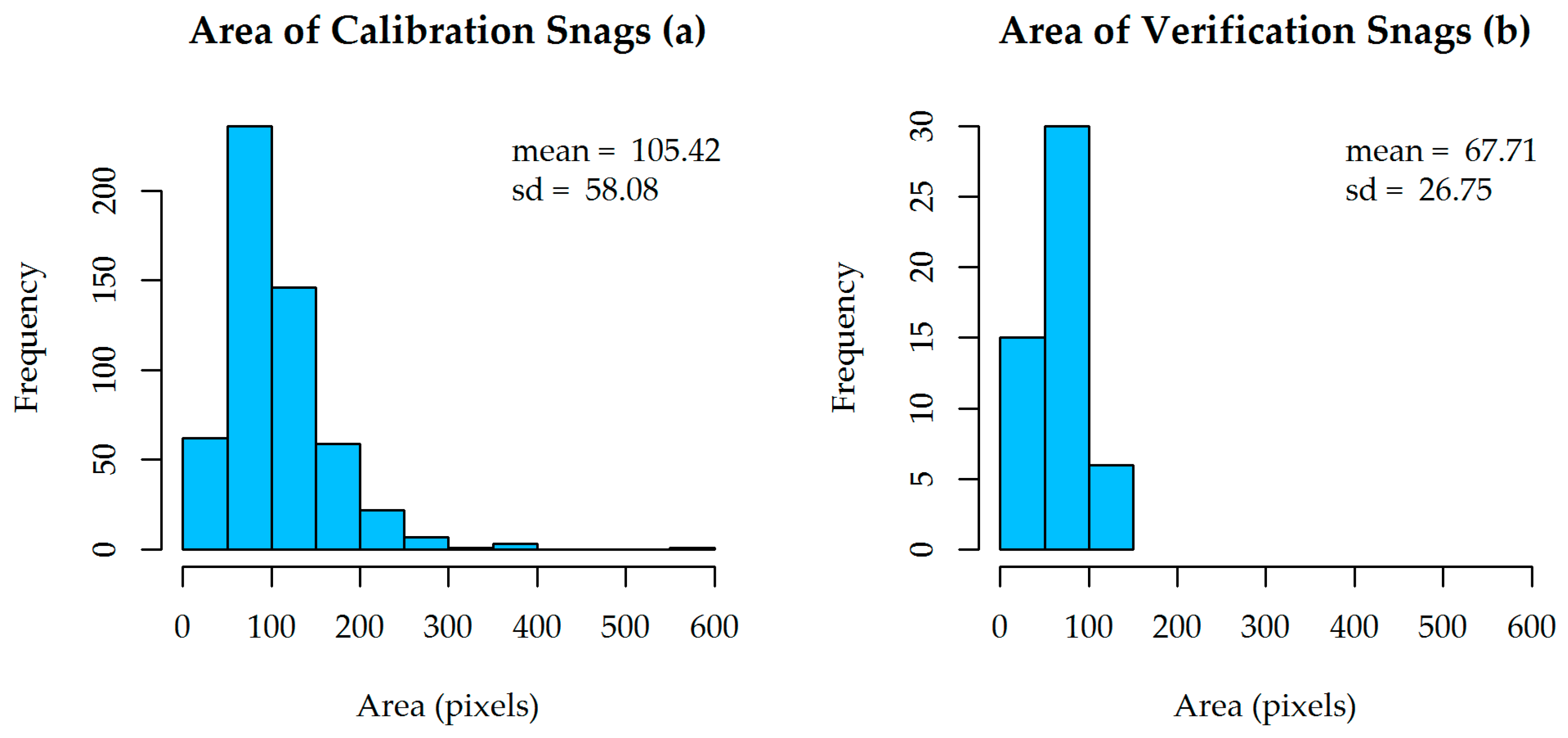
The considerable decrease in snag completeness between the calibration and verification tests in this study is likely due to the fact that most snags identified in the verification area were small coniferous trees, whereas most snags identified in the calibration area corresponded to medium to large sized conifers or large deciduous trees, as can be seen in the histograms of the area of snag objects (Figure 7). This highlights that the method is most effective when applied to an area with similar species compositions to the training area, or when ensured that the full range of composition is included in the training part.

The developed method was most accurate when mapping CWD regardless of the log/snag distinction, obtaining completeness and correctness for the CWD union class of 80.6% and 92.3%, respectively, in the verification area, and 93.4% and 94.5%, respectively, in the calibration area. These results support the observation that the workflow yields highly accurate detection of overall CWD given the complex and extensive nature of the study area. Since the accuracy metrics for the log and snag classes is significantly lower than for the CWD union class, it is evident that there is some confusion between log and snag objects. This suggests that there is room for improvement in the automated distinction between the CWD classes, which could be addressed in future studies.

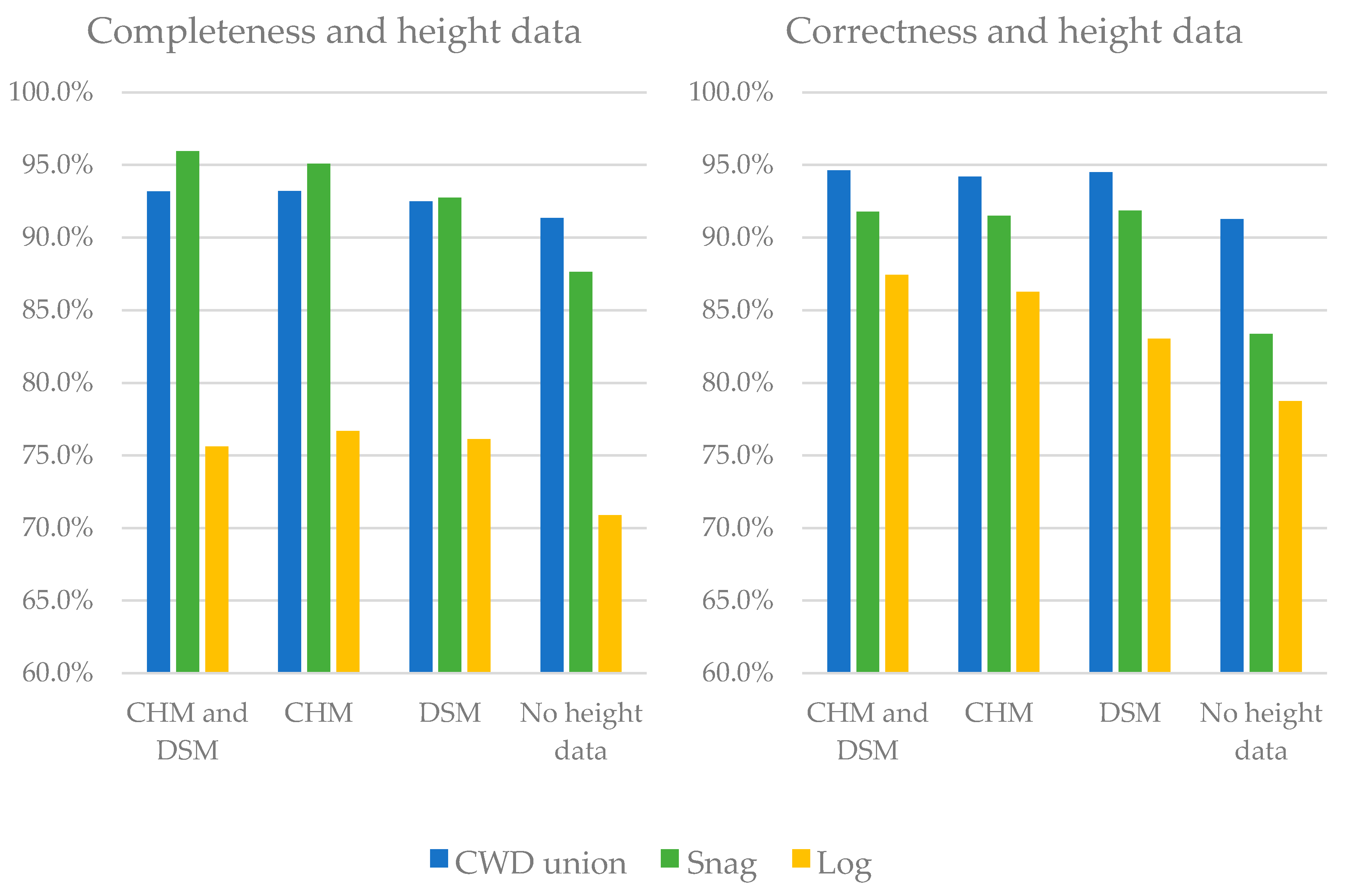
4.2. Significance of LiDAR-Derived Height Variables

Experiments using both, either, and none of the two types of height data—DSM and CHM—significantly increased the distinction between logs and snags, though the classification accuracy of the undistinguished CWD union improved by just 2%. We found the CHM to be significantly better than the DSM for the purpose of distinguishing logs from snags, particularly with respect to completeness. Although they theoretically present the same information, this difference might be due the fact that the dynamic data range in the CHM is larger (compared to the DSM), which is able to account for smaller variability of objects (heights).

There were no significant benefits of using both a DSM and a CHM. Since the CHM was derived from the DSM and a digital terrain model, the addition of DSM variables could be considered redundant in this case. The handling of redundant variables by the random forest algorithm is further discussed in the following subsection. We suggest that the most parsimonious selection of attributes concerning height data is the CHM, in addition to the spectral and shape attributes.

Future studies using similar methods that are not concerned with the distinction between logs and snags might choose to not use height data as predictor variables for CWD, since neither the CHM nor DSM significantly increased CWD union accuracy. Conversely, studies targeting snags or logs specifically, or concerned with the distinction between the two classes, will benefit from adding height data as predictor variables.

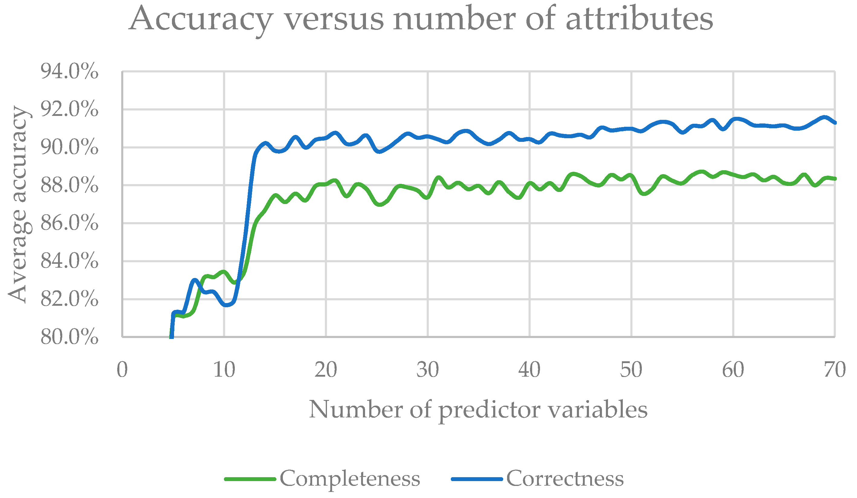
4.3. Importance of Predictor Variables

The NDVI was the most important predictor variable type overall, which was expected since CWD exhibits a very low NDVI signal overall. The top 15 attributes in the importance test included a mix of NDVI, spectral, spatial, and CHM variables, with DSM being the only variable type not included. This can be explained as random forest prioritizing CHM variables as better predictors than DSM for the target classes. However, one DSM-related variable was an outlier. DSM standard deviation ranked 18th place, while CHM standard deviation ranked 31st. It is possible that some of the local variability of the DSM was lost when subtracting a terrain model to generate the CHM, which could explain why RF ranks higher this one instance of DSM vs. CHM variables.

We found that accurate CWD detection could be achieved with as few as 15 predictor variables. As more attributes are added completeness seems to rise indefinitely, while correctness peaks around 45 attributes, after which it stabilizes around 88.5%. This effect suggests that RF is highly effective in boosting the effect of more important variables in its classification trees, minimizing the influence of redundant or ineffective variables.

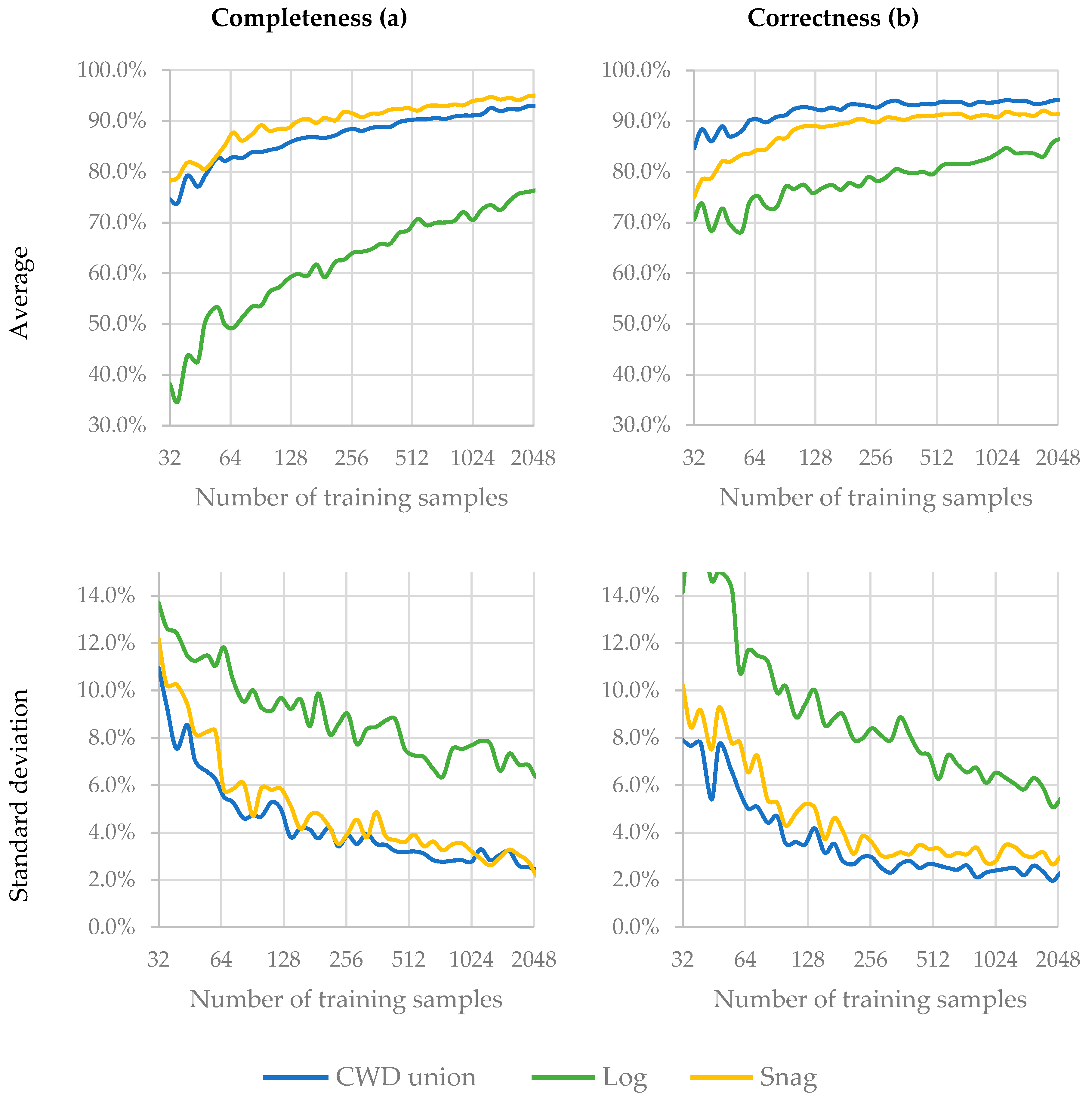
4.4. Effect of Training-Sample Size

Larger training-sample sizes yielded higher accuracy results, as expected. However, this effect seemed to be more drastic for the log class than the snag or CWD union classes. Since there were more snag samples (537) than log samples (364) in the calibration area, and since the number of samples in this experiment was decreased while maintaining the original proportion of samples for each class, it is logical to expect that the class with less samples will be more strongly affected when reducing the sample size. Completeness and correctness above 90% could be achieved in the CWD union class with as few as 512 samples. Good distinction between logs and snags, with accuracy metrics higher than 70%, could be achieved with about 1000 training samples.

4.5. Sources of Error

One important limitation to note is that the proposed method is only as reliable as the quality of the remote sensing data used, since blurriness, shadows, and occlusions can interfere with the identification of CWD. The accuracy tests performed in this study were based on what the human interpreter was capable to identify on the segmented orthomosaic, therefore human mistakes, as well as unidentifiable objects caused by small size, segmentation problems, and image processing artifacts, could not be fully accounted for in the accuracy assessments. These factors add a certain degree of uncertainty to our reported results. However, we consider the error sources related to pre-processing and segmentation to be minor relative to the number of meaningful identifiable objects in the images, as explained in Appendix A.

Some initial tests comparing leaf-on (summer) and leaf-off (spring) data of the study area suggested that there are trade-offs in accuracy when using either. Leaf-on has the advantage of much stronger NDVI contrast between live and dead vegetation, increasing the correctness of CWD detection. Leaf-off enables a more complete view of logs, since the occlusion caused by canopy is lessened, increasing the completeness of CWD detection. In this study, we prioritized correctness and used leaf-on data; future studies may compare and combine data obtained at different times for an assessment of the best configuration of input images for CWD classification.

Given the variability built into the selection process of the training and testing samples, as well as the creation of the random forest classifier, we suggest that the accuracy metrics be considered alongside their respective standard deviations. For example, given the results of Table 1, and given the normal distribution of completeness and correctness for CWD union in the calibration area, test metrics could be expressed as 93.4 ± 4.2% and 94.5 ± 3.2%, respectively, 19 out of 20 times.

4.6. Application and Next Steps

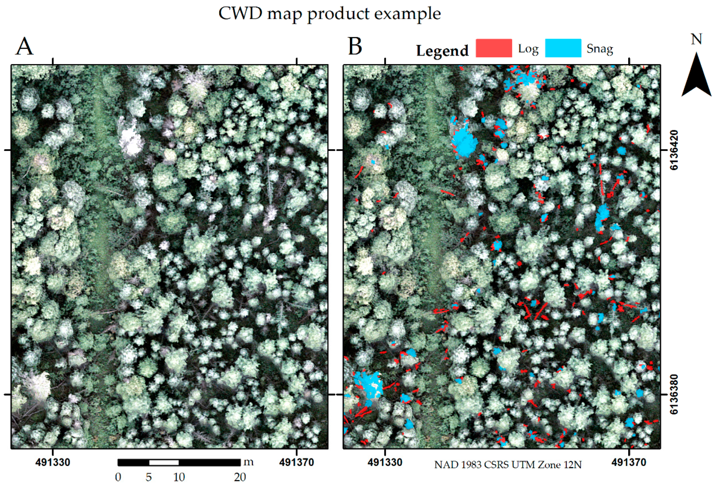
The developed method could be promptly applied to studies interested in CWD detection under any environmental context, be it forestry, biogeography, or disaster management. All that is required is for the user to possess aerial data of equivalent resolution to this study and produce a modest number (~100) of training samples. A sample CWD map, derived from a small subset of the study area, is shown in Figure 8.

Assuming that a hypothetical application area has similar variability in terms of CWD distribution and image-object attributes to the areas in this study, reliable accuracy could be expected by using the top 35 predictor variables listed in Appendix C. If an end user was not concerned with the distinction between logs and snags, then our experience suggest that a minimum of 100 training samples, assuming a NDVI-based random stratified sampling strategy, should suffice. If the distinction between logs and snags was important, then our results suggests that 1000 training samples would be required.

When applying this method to a different area, differences in CWD spatial distribution, species composition, class distribution, and climate will affect the accuracy of this method and importance of its predictor variables. The verification area test demonstrated that it is possible to apply a model developed in a different area of the same natural sub-region and overall structure without additional training and obtain reliable results. Studies outside of the boreal forest context or containing different unique features, such as an urban environment, should utilize their own training samples as explained above and expect similar results given an appropriate number of training samples. The more different the ecosystem of an application area is from the boreal context, the larger the anticipated difference between the results of this hypothetical application area and the results of this study in terms of accuracy, significance, and importance of predictor variables. However, given the robustness of random forests in prioritizing important variables based on the reference data, a new round of training on a hypothetical area should produce a random forest classifier well prepared for the specific features of this area. Additionally, the relative effect of transferability on classification accuracy, as observed in the verification area test, should be similar in different ecosystems when using a unique training set, assuming that these environments have similar within-ecosystem variability to the study area presented here.

This study achieved accurate detection of logs and snags in high-resolution (centimetric) images of an extensive and complex application area, located in the boreal forest of Alberta. We note the results in this paper are relative to what is visible in the input images. Occlusion caused by superimposed vegetation and visual ambiguities, such as similarities between live and recently dead trees or any other factor that may hinder manual visual identification of CWD objects, should also be expected to affect CWD detection based on supervised classification. For example, Inoue et al. (2014) evaluated manually identified remotely-sensed CWD relative to ground-truth and achieved about 85% completeness in a broadleaf forest of Japan. Further research could involve validating this method according to field-measured CWD and modelling the volume of the detected CWD objects, similar to Davis [29], but concerning both logs and snags in both forested and disturbed areas within the boreal application context.

5. Conclusions

We applied random-forest classification within a GEOBIA workflow to identify logs and snags in aerial four-band centimetric images (5.5 cm GSD) and LiDAR data (20 cm pixel CHM and DSM derived from 20 points/m² ALS) of the boreal forest. Great accuracy results—93.4 ± 4.2% completeness and 94.5 ± 3.2% correctness—were documented when training samples were present in the application area. Good accuracy results—80.6 ± 6.0% completeness and 92.3 ± 5.8% correctness—were found when training samples were detached from the application area. Experiments with CHM and DSM height variables as predictor variables revealed that even though height data did not increase overall CWD classification accuracy by more than 2% overall, it significantly improved the distinction between logs and snags. The CHM was significantly better than the DSM for this purpose. An attribute-importance test revealed that the most important predictor variables were a mix of NDVI, spectral, spatial, and CHM variables, and that a minimum of 15 attributes was required to obtain accurate classification. Adding more than 45 variables did not increase overall correctness. A test of training-dataset size showed that accurate results for the CWD union class could be achieved with as few as 512 training samples, but about 1000 samples were required to distinguish between logs and snags. Our results suggest that researchers, foresters, biogeographers, and government agencies can reliably make use of the developed workflow for mapping CWD on complex environments, such as the boreal forest of Alberta, and generate accurate products of strong ecological value.