Comparison of Horizontal Accuracy, Shape Similarity and Cost of Three Different Road Mapping Techniques

Abstract

Accurate spatial information on forest roads is important for forest management and harvest operations. This study evaluated the positional accuracy, shape similarity, and cost of three mapping techniques: GNSS (Global Navigation Satellite System) mapping, CAD file conversion (as-built drawing), and image warping. We chose five road routes within the national forest road system in the Republic of Korea and made digital road maps using each technique. We then compared map accuracy to reference maps made from field surveys. The mapping and field-survey results were compared using point-correspondence, buffering analysis, shape index, and turning function methods. The comparisons indicate that GNSS mapping is the best technique because it generated the highest accuracy (Root Mean Square Error: GNSS mapping 1.28, image warping 7.13, CAD file conversion 13.35), the narrowest buffering width for 95% of the routes overlapped (buffering width: GNSS mapping 1.5 m, image warping 18 m, CAD file conversion 24 m), highest shape similarity (shape index: GNSS mapping 19.6–28.9, image warping 7.2–10.8, CAD file conversion 6.5–7.4), and smallest area size difference in turning function analysis (GNSS mapping 2814–4949, image warping 7972–26,256, CAD file conversion 8661–27,845). However, GNSS requires more time (236 min/km) and costs more ($139.64/km) to produce a digital road map as compared to CAD file conversion (99 min/km and $40.90/km) and image warping (180 min/km and $81.84/km). Managers must decide on the trade-off between accuracy and cost while considering the demand and purpose of maps. GNSS mapping can be used for small-scale mapping or short-haul routes that require a small error range. Image warping was the lowest cost and produced low-accuracy maps, but may be suitable for large-scale mapping at the regional or national level. CAD file conversion was expected to be the most accurate method, because it converted as-built drawings to a map. However, we found that it was the least accurate method, indicating low accuracy of the as-built drawings. Efforts should be made to improve the accuracy of the as-built drawings in Korea.

1. Introduction

Forest roads are the infrastructure that affects accessibility to work sites that allow the continuation of forest management and harvest operations [1,2]. Forest roads are often considered an integral part of forest operations and, therefore, existing and new roads are either mapped or planned within the entire harvest operations platform. Because roads are essential for equipment and material movement, accurate spatial information on forest roads is crucial.

Forest maps are the most commonly used method to present spatial information. They can show terrain, land use, route position, land ownership, and stream channel networks. The display of this information requires current maps that are highly accurate [3,4]. Recently, with the advancement of computer technology, Geographic Information System (GIS) is widely used to analyze spatial information. In addition, thematic maps of forest vegetation, soil, and topography are now available in GIS [5]. In particular, GIS software is used to plan forest management activities that require a road network for planning and conducting forest operations [6]; necessitating a digital mapping system that is both accurate and cost-effective [2].

Spatial information for forest road mapping can be obtained in four ways: (i) digitizing after scanning of non-digital data (i.e., paper maps and as-built drawings); (ii) aerial photography and satellite imagery; (iii) field surveying; and (iv) data transference [7]. First, digitizing after scanning non-digital maps is highly efficient because it uses existing non-digital data. However, this type of mapping is impossible when non-digital data do not exist. Furthermore, periodic updates of non-digital data are required to maintain accuracy even if they do exist [4] and digitizing has the potential for errors caused by scaling or by the operator [7]. Second, aerial photography and satellite imagery are currently the most frequently-used methods for acquisition of spatial information due to their accuracy and efficiency, but it is expensive to obtain this data [8]. Third, field surveying is a time-consuming task and it is difficult to map a wide range of sites because data acquisition is performed by a few surveyors [6]. Fourth, data transference obtains spatial information by converting digital information through specific software such as GIS. This method is highly efficient as it can handle a wide range of spatial information at a given place [4,7], but it does not obtain information when there is no spatial data in a target area [4].

These methods for spatial information acquisition include a variety of detailed techniques, and the most representative techniques in terms of cost and time efficiency may be Computer Aided Design (CAD) file conversion [4,9], image warping [10,11] of as-built drawings, and Global Network Satellite System (GNSS) mapping [1,2]. The CAD file conversion technique utilizes digital as-built drawings with relatively up-to-date spatial information [8], and thus, it is easy to store, utilize and convert data on forest roads. The image warping technique is used for digital mapping of forest roads by calibrating image data on the as-built drawing based on the position coordinates established by GNSS surveys [11]. GNSS surveys are very useful in forest areas with a high-degree of roughness (i.e., complex topography, geology, and vegetation), and can produce relatively accurate and inexpensive thematic maps within a relatively small area [2,3].

Several studies [1,2,8,9] evaluated the accuracy of spatial information gathered from forest roads and compared the positional accuracy of GNSS field data collected from forest routes and its availability. GNSS mapping is considered a cost-effective tool to help manage and maintain forest road systems [1]. Kim et al. [9] produced digital maps of forest road networks using GNSS field data, satellite imagery, ortho-aerial photographs, and digital photogrammetry, and evaluated the positional accuracy and work efficiency. They concluded that the digital photogrammetric method was the most accurate although it required the greatest amount of time. In addition, advances in survey equipment, such as Airborne Laser Scanner (ALS) or Terrestrial Laser Scanner (TLS) obtain high-resolution spatial data, but this equipment has the disadvantage of a high cost to obtain data [8]. In recent years, 3D-based surveying technology was introduced to acquire precise and accurate spatial information. Both ALS and Structure from Motion (SfM) processing is being used to acquire spatial data based on a point-cloud for forest resource measurement [8,12]. For example, White et al. [8] measured the accuracy of log-haul roads and terrain using Light Detection and Ranging (LiDAR), generated Digital Terrain Models (DEMs), and evaluated the availability of Airborne LiDAR for spatial information on forest road and terrain.

The accuracy of digital maps can be evaluated by point-to-point positional comparisons [1,13] or shape similarity [14,15]. In order to evaluate the positional accuracy of a point object, the most commonly-used method is to determine the error (e.g., Root Mean Square Error (RMSE)) using a specific point or a corresponding point [1,13]. However, it is difficult to evaluate the accuracy and error range of features in linear or polygon form [14,16]. Therefore, many studies used RMSE of two- or three-dimensional coordinates to compare the geographical accuracy of linear objects such as roads [1,8,9]. In addition, methods have been developed to accurately evaluate the shape similarity or matching of linear or polygonal objects. This is similar to a buffering analysis that compares shape differences by evaluating the area size and shape of a polygon created by overlaying two objects [14,15] and the turning function by plotting the rotation angles and lengths of polygonal chains [17,18]. However, previous studies have only investigated the positional accuracy of each tool and none have compared both the positional accuracy and shape similarity of forest roads by digital mapping techniques, such as CAD file conversion, image warping, and GNSS mapping techniques. Without investigating these, the accuracy of these tools may not be fully evaluated.

Consequently, the aim of this study is to evaluate the horizontal accuracy, shape similarity, and cost of creating forest road maps using different mapping techniques. Specifically, we (i) made digital forest road maps using three techniques: (1) CAD file conversion, (2) image warping, and (3) GNSS mapping, and (ii) compared their accuracy, shape similarity time, and cost. The results of this study will contribute to improved long-term forest road maintenance, and road construction with a digital map of forest roads.

2. Materials and Methods

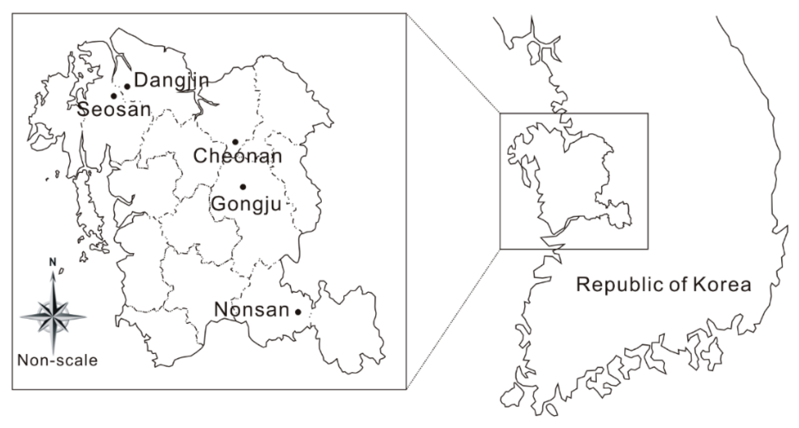
2.1. Study Area Description

This study consisted of five forest road routes that were located in Chungcheongnam-do in the Republic of Korea (Figure 1). The length of each route was 1–1.4 km (

Table 1. Information on study forest road routes.

Location	Length (m) 1	Construction Year	Altitude (m)				Forest Type
			B.P. 2	E.P. 3	Max.	Min.
Dangjin	1417	2009	147	190	190	143	Hardwood-forest
Seosan	1275	2008	116	98	124	97	Softwood-forest
Nonsan	1012	2009	151	154	175	151	Mixed forest
Choenan	1020	2007	174	197	197	167	Mixed forest
Gongju	1105	2009	401	412	447	397	Mixed forest

¹ Road length is the distance from as-built drawings. ² Beginning point. ³ End point.

) and were a part of the national forest road system of the Korea Forest Service (KFS). This study compares two-dimensional horizontal accuracy and, therefore, forest road sections with a small altitude difference were selected.

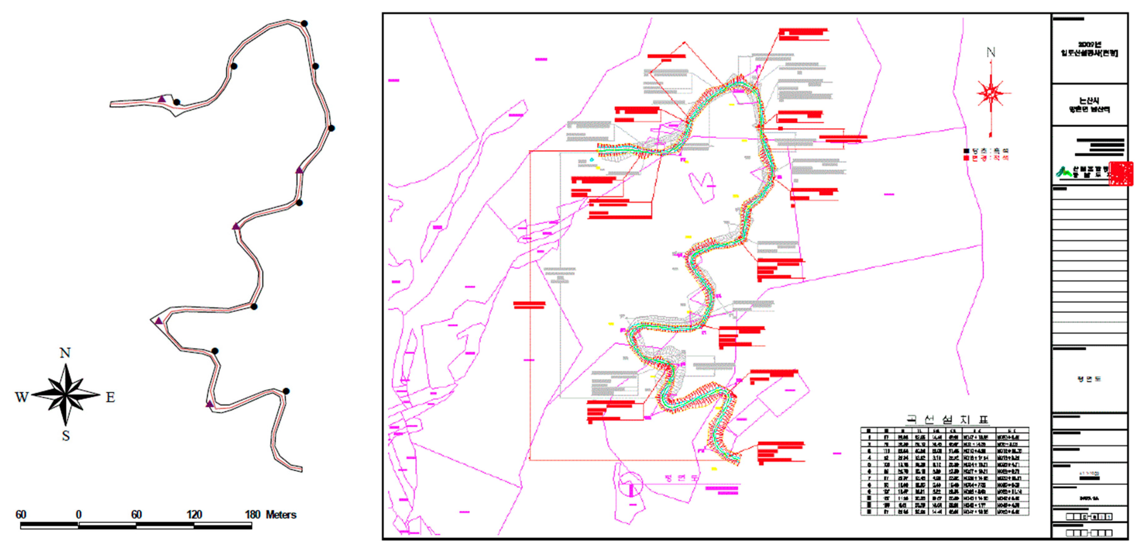
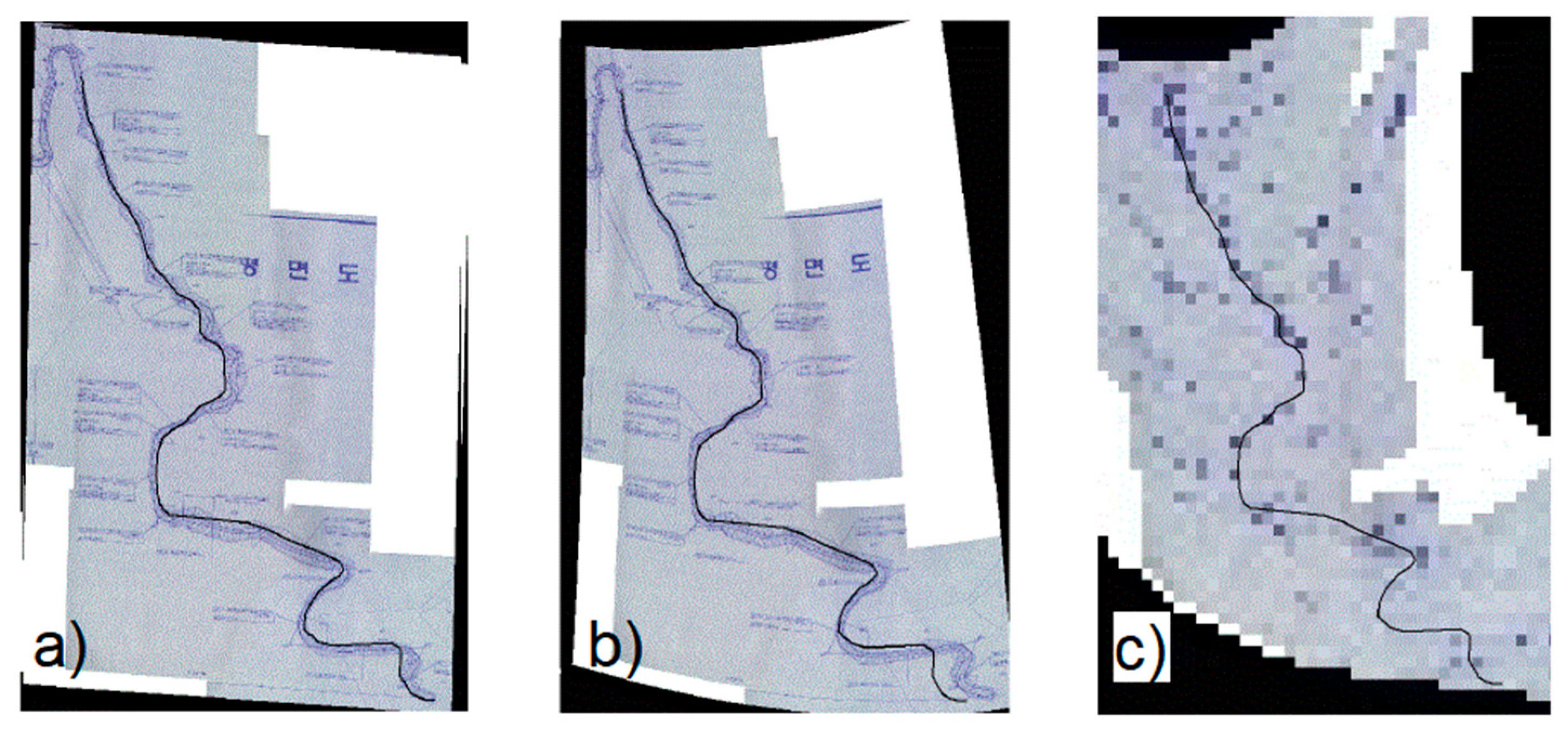
2.2. Mapping Techniques of Forest Roads

Digital road maps were made using three road-mapping techniques: (i) CAD file conversion, (ii) image warping, and (iii) GNSS mapping. Once mapping was complete, each method had their horizontal accuracies compared to the field-survey maps (i.e., reference maps) that were considered the most accurate (Figure 2, Figure S1). Development of a reference map was done with a SET530R Total Station (SOKKIA, Seoul, Korea) with an error range of ± 2 mm. This technique was used to measure the centerline and outline of the study routes. Reference maps were made using Power Comms [19] and AutoCAD [20].

The CAD file conversion technique created road maps using the as-built drawings, which comprised of CAD files without further enhancement (Figure 2). Only the objects related to the route were selected and converted to a CAD data file format (Drawing Exchange Format, DXF).

The CAD file conversion technique created road maps by scanning the as-built drawing files. The image warping technique used as-built drawings based on Ground Control Point (GCP). Image warping scanned and enhanced the blueprints from as-built drawings using the affine (linear) transformation [21] and image warp feature of ESRI ArcView® 3.2 [22]. We found that the affine transformation worked best for the image warping (Figure 3).

The GNSS mapping used a Pro-XRS (Trimble Corp., Sunnyvale, CA) to acquire route data that was downloaded and converted to the road maps using Pathfinder Office software [23] (Figure 4).

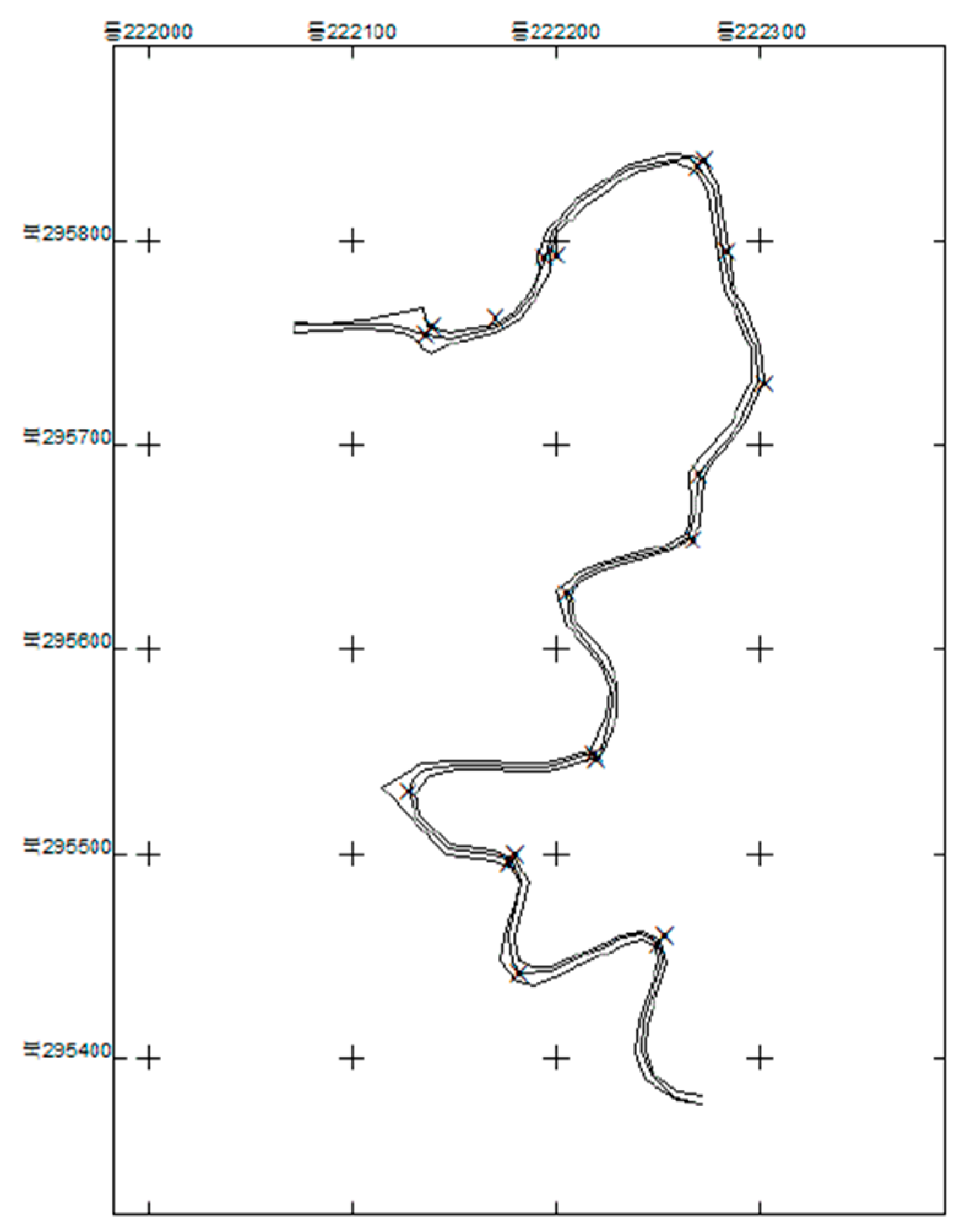
2.3. Comparison of the Horizontal Accuracy and Shape Similarity between Three Mapping Techniques

Four methods were used to evaluate the horizontal accuracy and shape similarity between the three mapping techniques: (1) point-correspondence [13,24,25], (2) buffering analysis [14,15], (3) shape index [26], and (4) turning function [17,27]. We only investigated the horizontal positional accuracy because that is more important than vertical accuracy, since most maps are shown in the horizontal plane.

2.3.1. Point-Correspondence

Point-correspondence accuracy is based on the corresponding point to evaluate a difference between the same points using different techniques. An error is determined using Root Mean Square Error (RMSE) based on the deviation between the two points on the x- and y-axes [13,24,25]. Therefore, a single RMSE on the plane position can be calculated as follows:

$$rmse=\sqrt{{\left(rms{e}_x\right)}^2+{\left(rms{e}_y\right)}^2}$$

(1)

where:

• rmse_x is root mean square error of x-axis,
• rmse_y is root mean square error of y-axis.

We selected 49 corresponding points from the five forest road routes and calculated RMSE values by the mapping technique and study site location. The results were statistically analyzed with a two-tailed t-test using a significance level of 0.01.

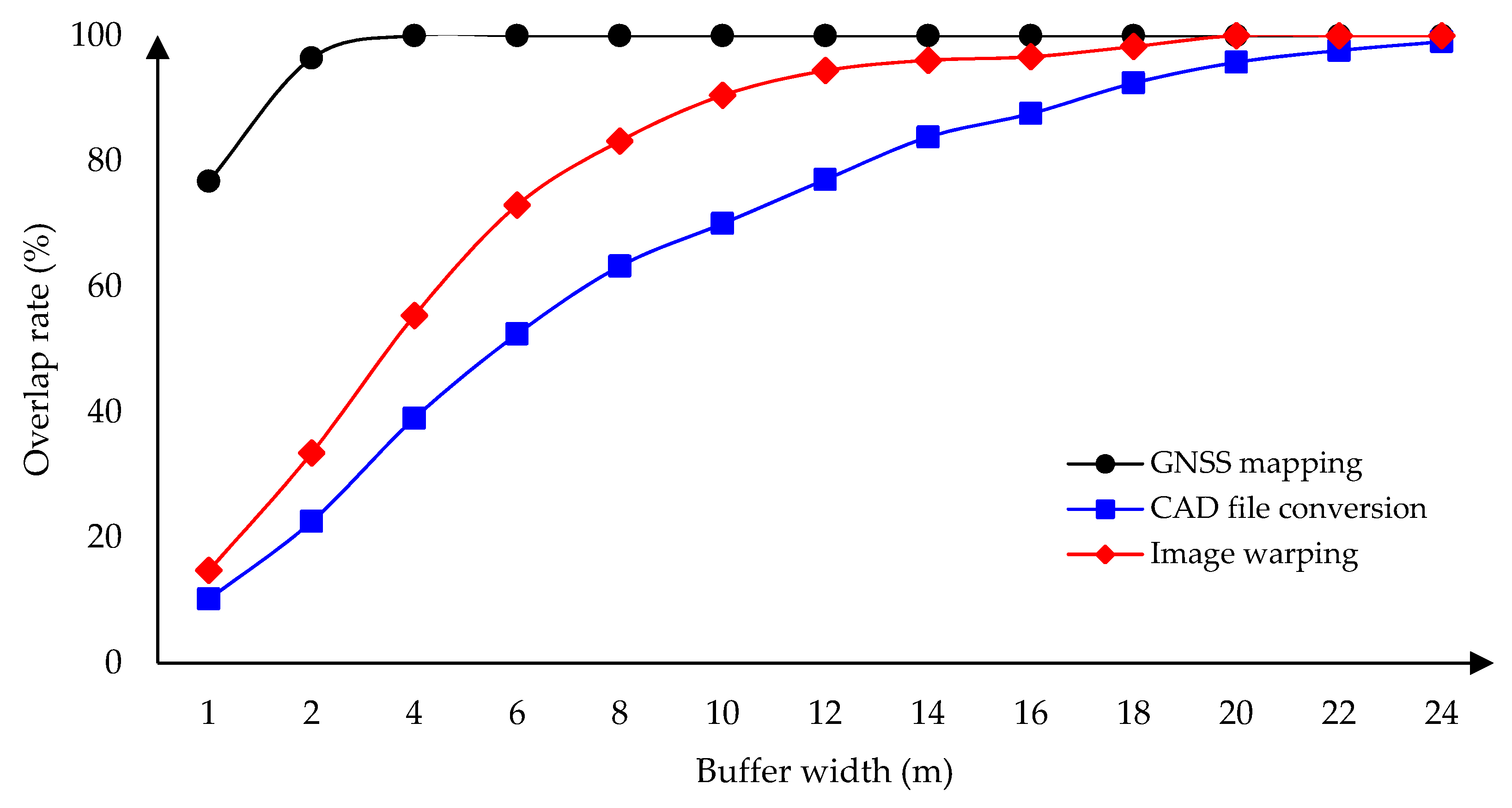
2.3.2. Buffering Analysis

It is very difficult to define the accuracy of vector data on unequal locations. Buffering methods are used to compare the accuracy of linear objects that do not correspond to each other [14,15]. We buffered the reference route at 2 m intervals, calculated the buffer width using 95% of the comparable routes, and compared the buffer widths by the mapping technique.

2.3.3. Shape Index

Buffering methods evaluate map accuracy through proximity to lines that do not correspond to each other, but the similarity of shapes cannot be determined. Therefore, it is necessary to further compare the similarity of the shapes of the study routes. Shape index is a method of comparing shapes as an index used to calculate the shape ratio. It is expressed as a ratio of area to circumference length [28]. Shape index was calculated for the polygon generated from the buffering analysis. If the shape was circular, the shape index is one (i.e., the small perimeter in a given internal area). If the shape was square, the shape index is 1.13. The shape index can be expressed as follows [15]:

$$D_i=\frac{p}{2\sqrt{A\pi }}$$

(2)

where:

• $D_i$: shape index,
• p: perimeter (m),
• A: Area (m²).

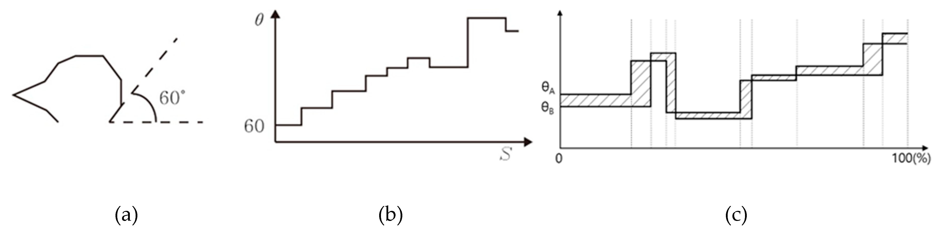
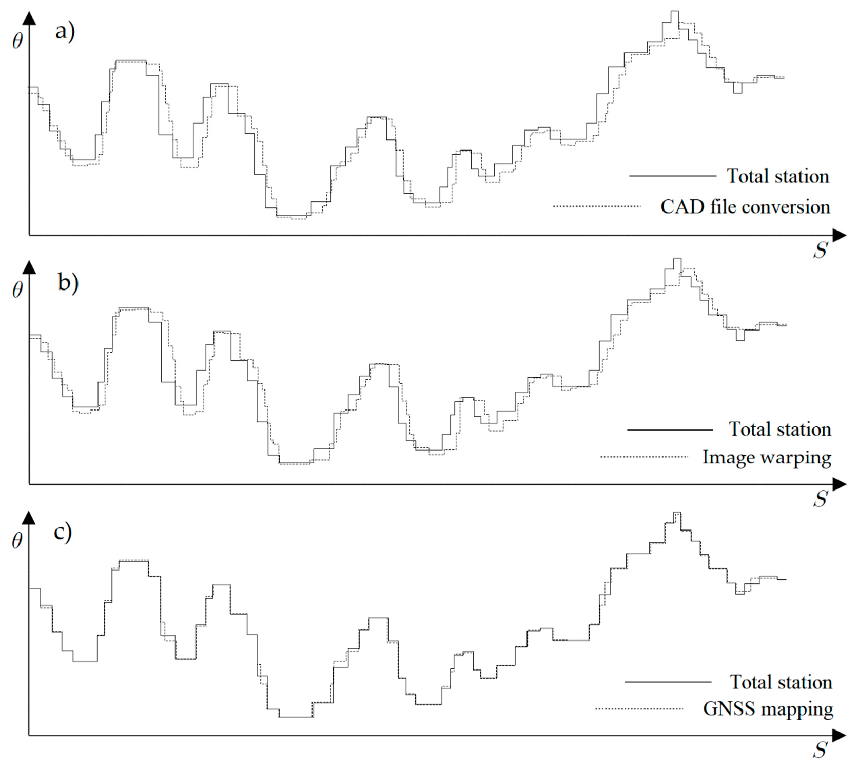
2.3.4. Turning Function Analysis

Turning function analysis is another method to compare the shape differences of objects, by plotting the rotation angles and lengths of polygonal chains [17,18]. It typically uses a graph that has the x-axis as the length of the comparing object and the y-axis as the rotation angle. Thus, the x-axis depends on the chain length. The y-axis value increases as the rotation angle of the chain increases, and decreases as the rotation angle decreases.

We had one reference map and three maps from each mapping technique. Therefore, the total lengths of polygonal chains might vary depending on the mapping technique. In order to only compare shape similarities, the total length was set to 100% and the ratio of each polygonal chain length was calculated [17,27]. After that, the rotational angles and ratios of polygonal chain lengths were plotted (Figure 5a,b). The shape similarities were compared by calculating the area difference between the graphs plotted from the reference map and three mapping techniques (Figure 5c). The area difference between two graphs is a relative value, and therefore a lower value indicates a higher shape similarity.

2.3.5. Estimation of Map-Making Time and Cost

The working time of the three mapping techniques was estimated by measuring the time spent on the field survey and digital map-making of the five road routes. We determined the labor cost [29] and work time to estimate the total cost. Worktime and cost are presented as an average cost per unit road length (US dollar/km).

3. Results

There were differences in route length between the maps created when using the total station and three mapping techniques (

Table 2. Comparisons of the study route length by mapping technique.

Area	No. of IP 1 (ea)	Total Station (m)	CAD File Conversion (m)	Image Warping (m)	GNSS Mapping (m)
Dangjin	11	1398	1417 (△19)	1438 (△40)	1396 (▽2)
Seosan	19	1209	1275 (△66)	1280 (△71)	1211 (△2)
Nonsan	12	985	1012 (△27)	1040 (△55)	986 (△1)
Cheonan	13	1048	1020 (▽28)	1123 (△75)	1047 (▽1)
Gongju	23	1022	1105 (△83)	1101 (△79)	1027 (△5)
Total	78	5662	5829 (△167)	5982 (△320)	5667 (△5)

¹ Intermediate point.

). The Total Station data indicated that the length of the study area was 5662 m. This was shorter than the lengths produced by both the CAD file and image warping, but very similar to GNSS mapping.

3.1. Point-correspondence

After analyzing 49 points along the surveyed routes, the average RMREs from CAD file conversion, image warping, and GNSS mapping were 13.53 m, 7.13 m, and 1.28 m respectively, indicating that the GNSS mapping accuracy is the highest (

Table 3. Comparison of point-correspondence results (RMSE) by mapping technique.

Mapping Technique	Total		Dangjin		Seosan		Nonsan		Cheonan		Gongju
	Mean	SD 1	Mean	SD	Mean	SD	Mean	SD	Mean	SD	Mean	SD
CAD file conversion	13.35 a	7.36	14.78 c	9.38	14.51 c	6.25	11.04 c	4.52	13.07 c	6.86	14.01 c	7.68
Image warping	7.13 b	3.75	8.79 b	3.34	8.97 b	3.66	5.63 b	2.49	5.66 b	3.06	6.46 b	4.16
GNSS mapping	1.28 c	0.86	1.99 a	0.63	0.81 a	0.48	1.08 a	0.64	1.16 a	0.82	1.36 a	1.00
F	79.89		11.10		24.28		22.08		17.08		14.14
P	< 0.01		< 0.01		< 0.01		< 0.01		< 0.01		< 0.01

¹ SD: Standard deviation. Superscript letters (a, b, and c) next to means represent significant difference at α = 0.01.

). In particular, CAD file conversion had 10.4 times the mean and 8.56 times the standard deviation of the RMSE as compared to GNSS mapping.

The positional accuracy (RMSE) of the image warping is about 47% as compared to the CAD file conversion, indicating that image warping is more accurate than the CAD file conversion. For all five study routes, the RMSEs were significantly different.

3.2. Buffering Analysis

In the buffering analysis, overlaying the CAD file conversion maps on top of the reference maps resulted in a buffer width of 24 m, and greater than 95% of routes being included in the buffer range. Buffer widths, when overlapping 95% of the routes, were as follows: Gongju (16 m), Dangjin (18 m), Nonsan (18 m), Cheonsan (22 m), and Seosan (24 m) (Figure S2). Overlaying the image warping and reference maps indicated that with a buffer width of 18 m, more than 95% of the routes were included in the buffer range (Figure S3). Buffer width, when overlapping 95% of the routes, were as follows: Nonsan (10 m), Dangjin (12 m), Cheonsan (12 m), Gongju (18 m) and Seosan (18 m). GNSS mapping allowed the use of the narrowest buffer width (Figure 6). On average, more than 95% of the routes were included in the buffer range of the reference map when the buffer width was 1.5 m. When the all routes (100%) were included, buffer widths were 4 m (Figure S4).

3.3. Shape Index

The shape index of the converted CAD file was 6.5–7.4, image warping was 7.2–10.8, and GNSS mapping was 19.6–28.9 (

Table 4. The shape index by mapping technique.

Route Location	Mapping Technique	Area (m2)	Length (m)	Shape Index
Dangjin	CAD file conversion	11,715	2839.7	7.4
	Image warping	5548	2852.8	10.8
	GNSS mapping	1624	2800.0	19.6
Seosan	CAD file conversion	11,884	2506.6	6.5
	Image warping	6733	2503.9	8.6
	GNSS mapping	557	2422.0	28.9
Nonsan	CAD file conversion	6040	2019.4	7.3
	Image warping	3517	2037.1	9.7
	GNSS mapping	554	1974.0	23.7
Cheonan	CAD file conversion	6942	2123.8	7.2
	Image warping	4582	2194.1	9.1
	GNSS mapping	479	2099.0	27.0
Gongju	CAD file conversion	8612	2165.4	6.6
	Image warping	7169	2164.2	7.2
	GNSS mapping	681	2042.0	22.1

). As previously noted, when the shape of the measured polygon is circular the shape index is 1. The index increases when the shape elongates (e.g., becomes bar-shaped) [26]. Therefore, a higher index indicates that the shape is closer to the reference map. In general, polygons from GNSS mapping results in a shape index greater than 20, indicating narrow and long shapes more closely resembling the reference map. In contrast, the shape indices from the CAD file conversion and image warping methods resulted in shape indices that were generally less than 10, indicating broader shapes and less shape similarity to the reference map.

3.4. Turning Function Analysis

Differences in mapped area size among the three mapping techniques as compared to the reference map were as follows: CAD file conversion (8661–27,845), image warping (7972–26,256), and GNSS mapping (2814–4949) (

Table 5. Area size difference in turning function analysis between the three mapping techniques and reference map.

Route Location	Mapping Technique
	CAD File Conversion	Image Warping	GNSS Mapping
Dangjin	8661	7972	3357
Seosan	19,633	16,984	3230
Nonsan	14,211	13,994	2814
Cheonan	23,588	19,331	4130
Gongju	27,845	26,256	4949

, Figure 7, Figures S5–S8). Overall, the mapped area differences were lowest using GNSS mapping, followed by image warping, and CAD file conversion. Our results indicate that the GNSS mapping produced maps that were most similar to the reference map.

3.5. Estimation of Map-Making Time and Cost

The working time of three mapping techniques, inclusive of field survey and map-making, were 236 min/km for GNSS mapping, 180 min/km for image warping, and 99 min/km for CAD file conversion. Production costs to create a digital map were $139.64/km for GNSS, $81.84/km for image warping, and $40.90/km for CAD file conversion, indicating that CAD file conversion was the most cost-efficient (

Table 6. Time study and cost analysis of forest road digital map by three mapping techniques.

Mapping Technique	Average Working Time (min/km)			Production Cost (US$/km) 3
	Field Survey 1	Map-making 2	Total
CAD file conversion	-	99	99	40.90
Image warping	31	149	180	81.84
GNSS mapping	175	61	236	139.64
Total station	195	120	315	180.66

¹ Conducted by one experienced technician ($175.47/day) and one beginner technician ($138.25/day). ² Conducted by one expert technician ($198.22/day). ³ Converted from Korean Won (₩) based on 2018 currency exchange rate [30].

). In addition, the working time to produce the reference map using the total station was 315 min/km (195 min/km for on-site survey and 120 min/km for map-making work), and the total cost was $180.66/km.

4. Discussion

Map accuracy is one metric for determining the best mapping method and, for our study, map accuracy followed the trend (from greatest to smallest) of GNSS, image warping, and CAD file conversion. However, there are several error-sources inherent within spatial data that should be addressed before making a digital map using GIS or CAD programs. In the forest environment, the constraints of surveying include difficult terrain and trees taller than the user, but GNSS is primarily used because of convenience and efficiency [1,2,31]. Many studies have shown, however, that the accuracy of GPS-based surveying has an error range of 1–88 m [2,8] and depends on the user and/or receiver environment. In particular, the failure to receive satellite signals because they are blocked by a forest canopy or hilly terrain during forest road route surveys is one possibility of user error [1]. Therefore, in order to increase the accuracy of GPS surveying, it is necessary to reduce the influence of the forest canopy and terrain, to have enough time to receive satellite signals, and to educate and train users to reduce human error [1,32]. Scanning and data transferring methods such as image warping and CAD file conversion might also have an error of positional accuracy due to the data itself. For example, during road construction changes made in the route are often not reflected in the as-built drawings. After completion of road construction, the as-built drawings are made using blueprints rather than conducting field surveys again. We considered data inaccuracy as a part of the overall methodological errors, due to lack of detailed field survey data after the road construction. Future studies are needed to further assess the different errors associated with image warping and CAD file conversion.

In many forest studies the positional accuracy was evaluated by measuring the difference between a known reference point and the corresponding points, and then calculating the position error (e.g., RMSE). However, it is difficult to compare the morphological differences of line segments [14,16] because mid- and endpoints in a line segment can contain disproportionate error terms [33]. Furthermore, since linear networks, such as roads, often do not have adequate comparison points, it may be more appropriate to simply compare features within a road network to a more accurate, linear reference [14,15] or to internal digital geometry [24,34,35].

Shape matching is important for comparing accuracy and similarity [18], especially for a line or polygon segment such as the centerline of roads, railways, shorelines, and boundaries of natural phenomena [15]. Thus, we used the highly accurate reference map to compare the positional accuracy and shape similarity of the other mapping methods by using point-correspondence and buffering analysis. The results from both methods showed that GNSS mapping was the most accurate technique. However, this method also takes more time and has a greater associated cost to collect field data and construct maps as compared to the other two techniques. For the CAD file conversion technique, the only time requirement was to input or edit locations and information on the forest road routes and facilities without the need for a field survey. Therefore, it took 42% less field and mapping time and had 27% less cost as compared to GNSS. Image warping took more time than the CAD file conversion because it required a field survey to obtain the GCP and additional processing time to scan the drawings.

This study reports high GNSS time and costs and is similar to findings of previous studies. Kim et al. [9] reported it took 17 h to measure 35 km of forest road routes using a GPS receiver, while it took 6 h using aerial imagery. Furthermore, Ömer & Ayhan [7] reported that the production cost of GNSS mapping for spatial information ($17.22/ha) was about 3.6 times that of the digitizing method ($4.79/ha).

LiDAR is a widely used remote sensing technology that can be used as a road mapping method [8,36]. In Korea, road map-making using LiDAR costed $11.05/ha for 1:1000 map and $7.10/ha for 1:5000 map [30,37], which are less than GNSS but greater than the digitizing method [7]. Future studies are needed to assess more up-to-date map-making technologies for forest road, such as LiDAR and 3D-based geographical information using point-cloud.

If higher map-making accuracy is required, then there will be associated increase in mapping costs. Similarly, if mapping funds are limited, map accuracy will be lower [9]. Therefore, it is necessary to make decisions regarding the trade-off between accuracy and cost, while considering the demand and purpose of maps. GNSS mapping techniques are most suitable for small-scale mapping or short-haul routes where a small error range is required (e.g., less than 1m). CAD file conversion can be accurate because it converts as-built drawings with high accuracy into a map. However, this study found that the data did not match well with the reference map and the technique was less accurate than GNSS mapping. In Korea, more efforts should be made to improve the accuracy of the as-built drawings and CAD file conversion. Due to their lower level of accuracy, CAD file conversion is recommended for making a large-scale road inventory at the regional or national level. Due to low accuracy, the image warping technique can also be considered for large-scale mapping or long-distance routes, such as 1:25,000 or greater.

This study compared the horizontal accuracy of different mapping techniques in forested areas in Korea. Considering that most maps are shown in the horizontal plane, we did not include vertical accuracy in this study. However, Korea has steep terrains [38], and vertical accuracy might be of importance and is worth future investigations.

5. Conclusions

This study compared the horizontal accuracy, shape similarity, and production cost of creating forest road maps using different mapping techniques (i.e., CAD file conversion, image warping, and GNSS mapping) to determine the most effective methods to produce digital forest road maps. We conclude that GNSS mapping is the best technique when considering high accuracy and shape similarity. GNSS mapping, however, requires a substantial amount of time and considerable costs to produce digital maps. Therefore, GNSS mapping should be used for small-scale mapping or short-haul routes that require a small error range, while CAD file conversion and image warping can be used for large-scale mapping. CAD file conversion has been shown to be relatively accurate, but our data did not match well with the reference map and were less accurate than GNSS mapping. Since this method is less expensive and can produce maps suitable for long distances (large areas), greater effort should be made to improve the accuracy of the CAD file conversion in Korea. In addition, the accuracy of GPS surveying for GNSS mapping can be increased by educating and training users on how to reduce the influence of the forest canopy and terrain, while ensuring that there is enough time to receive satellite signals.

Effective forest management and harvest operations require precise spatial information. This study contributes knowledge about how to improve forest road mapping accuracy. There are increasing interests and needs (e.g., earthwork, cut and fill) for 3D-based geographical information using point-cloud. In the future, it will be necessary to make 3D road maps from point-cloud based data and to utilize this to develop an effective and efficient road inventory for large aerial extent mapping projects in mountainous areas.

References

1. Abdi, E.; Sisakht, L.; Goushbor, L.; Soufi, H. Accuracy assessment of GPS and surveying technique in forest road mapping. Ann. For. Res. 2012, 55, 309–317. [Google Scholar]
2. Talebi, M.; Majnounian, B.; Ehsan, A.; Tehrani, F.B. Development a GIS database for forest road management in Arasbaran forest, Iran. For. Sci. Technol. 2015, 11, 27–35. [Google Scholar] [CrossRef]
3. Murphy, P.N.C.; Ogilvie, J.; Castonguay, M.; Zhang, C.F.; Meng, F.R.; Arp, P.A. Improving forest operations planning through high-resolution flow-channel and wet-areas mapping. For. Chron. 2008, 84, 568–574. [Google Scholar] [CrossRef] [Green Version]
4. Yang, S.; Choi, J.; Yu, K. Development of the Digital Map Updating System using CAD Object Extracted from As-Built Drawings. J. Korean Soc. GIS 2009, 17, 13–21, (In Korean with English Abstract). [Google Scholar]
5. Alizadeh, S.; Majnounian, B.; Darvishsefat, A. Possibility of designing and evaluation of forest road network variants using GIS and field investigation. J. For. Wood Prod. 2011, 63, 399–408. [Google Scholar]
6. Grigolato, S.; Mologni, O.; Raffaele, C. GIS applications in forest operations and road network planning: An overview over the last two decades. Croat. J. For. Eng. 2017, 38, 175–186. [Google Scholar]
7. Ömer, M.; Ayhan, C. Accuracy and cost comparison of spatial data acquisition methods for the development of geographical information systems. J. Geogr. Regional Plan. 2009, 2, 235–242. [Google Scholar] [CrossRef]
8. White, R.A.; Dietterick, B.C.; Mastin, T.; Strohman, R. Forest roads mapped using LiDAR in steep forested terrain. Remote Sens. 2010, 2, 1120–1141. [Google Scholar] [CrossRef]
9. Kim, T.; Yoon, J.; Woo, C.; Lee, K.; Hong, C. Comparison of methodology and accuracy of digital mapping of forest roads. J. Geogr. Inform. Syst. Assoc. Korea 2005, 13, 195–209. (In Korean) [Google Scholar]
10. Glasbey, C.; Mardia, K. A review of image warping methods. J. Appl. Stat. 1998, 25, 155–171. [Google Scholar] [CrossRef]
11. Kim, M.; Kweon, H.; Choi, Y.; Yeom, I.; Lee, J. Evaluation of horizontal position accuracy in forest road completion drawing. Korean J. Agr. Sci. 2010, 37, 471–479, (In Korean with English Abstract). [Google Scholar]
12. Wallace, L.; Lucieer, A.; Malenovský, Z.; Turner, D.; Vopěnka, P. Assessment of Forest Structure Using Two UAV Techniques: A Comparison of Airborne Laser Scanning and Structure from Motion (SfM) Point Clouds. Forests 2016, 7, 62–78. [Google Scholar] [CrossRef]
13. Kagawa, Y.; Sekimoto, Y.; Shibasaki, R. Comparative study of positional accuracy evaluation of line data. In Proceedings of the 20th Asian Conference on Remote Sensing, Hong Kong, China, 22–25 November 1999. [Google Scholar]
14. Goodchild, M.; Hunter, G. A simple positional accuracy measure for linear features. Int. J. Geogr. Inform. Sci. 1997, 11, 299–306. [Google Scholar] [CrossRef]
15. Tveite, H.; Langaas, S. An accuracy assessment method for geographical line data sets based on buffering. Int. J. Geogr. Inform. Sci. 1999, 13, 27–47. [Google Scholar] [CrossRef]
16. Lueng, Y.; Yan, J. A locational error model for spatial features. Int. J. Geogr. Inform. Sci. 1998, 12, 607–620. [Google Scholar] [CrossRef]
17. Arkin, E.; Chew, P.; Huttenlocher, D.; Kedem, K.; Mitchel, J. An efficiently computable metric for comparing polygonal shapes. IEEE Trans. Pattern Anal. Mach. Intell. 1991, 13, 209–215. [Google Scholar] [CrossRef]
18. Velkamp, R.C. Shape matching: similarity measures and algorithms. In Proceedings of the International Conference on Shape Modeling and Applications, Genova, Italy, 7–11 May 2001. [Google Scholar]
19. SOKKIA KOREA. Available online: https://www.sokkia.co.kr (accessed on 15 August 2010).
20. AutoCAD. Available online: https://www.autodesk.com (accessed on 15 April 2012).
21. Parkhomenko, A.S. Affine transformation. In Encyclopedia of Mathematics; Hazewinkel, M., Ed.; Springer: Berlin, Germany, 2010; Available online: http://www.encyclopediaofmath.org/index.php?title=Affine_transformation&oldid=17980 (accessed on 9 September 2018).
22. ESRI. Available online: http://support.esri.com (accessed on 15 August 2010).
23. Trimble Korea. Available online: https://geospatial.trimble.com (accessed on 15 June 2010).
24. Van Niel, T.G.; McVicar, T.R. Experimental evaluation of positional accuracy estimates from a linear network using point-and line-based testing methods. Int. J. Geogr. Inform. Sci. 2002, 16, 459–473. [Google Scholar] [CrossRef]
25. Ramirez, J.R.; Ali, T. Progress in metrics development to measure positional accuracy of spatial data. In Proceedings of the 21st International Cartographic Conference, Durban, South Africa, 10–16 August 2003; pp. 1763–1772. [Google Scholar]
26. Forman, R.T.T.; Godron, M. Landscape Ecology; John Wiley and Sons: New York, NY, USA, 1986; pp. 188–189. [Google Scholar]
27. Velkamp, R.C.; Hagedoorn, M. Shape similarities, properties, and constructions. In Proceedings of the 4th International Conference, Lyan, France, 2–4 November 2000; pp. 467–476. [Google Scholar]
28. Kim, M.; Ahn, D. Landscape ecological analysis of urban parks –analysis of index of patch shape and the dispersion of patches. J. Korean Inst. Landsc. Archit. 1996, 23, 12–19, (In Korean with English Abstract). [Google Scholar]
29. Korea Engineering and Consulting Association (KENCA). Available online: https://www.etis.or.kr/webs/statistics/statistics_board.jsp?leftParam=1&topParam=3&boardId=TOTALBBS&categorygroup2=TB050 (accessed on 6 May 2019).
30. KEB Hanabank. Available online: https://www.kebhana.com (accessed on 14 January 2019).
31. Pirti, A. Accuracy analysis of GPS positioning near the forest environment. Croat. J. For. Eng. 2008, 29, 189–199. [Google Scholar]
32. Yosimura, T.; Hasegawa, H. Comparing the precision and accuracy of GPS positioning in forested areas. J. For. Res. 2003, 8, 147–152. [Google Scholar] [CrossRef]
33. Shi, W. A generic statistical approach for modelling error of geometric features in GIS. Int. J. Geogr. Inform. Sci. 1998, 12, 131–143. [Google Scholar] [CrossRef]
34. Duckham, M.; Drummond, J. Assessment of error in digital vector data using fractal geometry. Int. J. Geogr. Inform. Sci. 2000, 14, 67–84. [Google Scholar] [CrossRef] [Green Version]
35. Veregin, H. Quantifying positional error induced by line simplification. Int. J. Geogr. Inform. Sci. 2000, 14, 113–130. [Google Scholar] [CrossRef]
36. Azizi, Z.; Najafi, A.; Sadeghian, S. Forest road detection using LiDAR data. J. For. Res. 2014, 25, 975–980. [Google Scholar] [CrossRef]
37. Kang, J.M.; Yoon, H.C.; Lee, J.D.; Park, J.K. Analysis of economical efficiency of digital map in production cost by aerial LiDAR surveying. J. KOGSIS 2007, 15, 67–73, (In Korean with English Abstract). [Google Scholar]
38. Yang, B. Republic of Korea, Nation Map Book II; Ministry of Land, Infrastructure and Transport, National Geographic Information Institute: Suwon, Gyeonggi-do, Korea, 2016. Available online: http://map.ngii.go.kr/ms/pblictn/nationMapBook.do (accessed on 17 September 2018).
Figure 1. Study site locations.
Forests 10 00452 g001
Figure 2. Examples of the reference map using the total station (left, ▴ GCP, centerline of forest road) and conversion from the as-built drawing file to DXF file format (right).
Forests 10 00452 g002
Figure 3. Examples of image warping using blueprints and GCP: (a) 1st transformation (linear), (b) 2nd transformation, (c) 3rd transformation. The image warping effect decreases when using the 2nd and 3rd transformations.
Forests 10 00452 g003
Figure 4. An example of GNSS mapping.
Forests 10 00452 g004
Figure 5. Turning function analysis: (a) calculating rotational angles and polygonal chain length, (b) plotting rotational angles and ratios of polygonal chain lengths, and (c) comparing shape similarities by calculating the area difference.
Forests 10 00452 g005
Figure 6. Results of buffering analysis by mapping technique. The overlapping rates were average values.
Forests 10 00452 g006
Figure 7. Example of turning function analysis between the three mapping techniques and reference map on Nonsan: (a) CAD file conversion, (b) image warping, and (c) GNSS mapping.
Forests 10 00452 g007