Influence of 3D Spruce Tree Representation on Accuracy of Airborne and Satellite Forest Reflectance Simulated in DART

 , ,
, ,  , ,
, ,
Abstract
1. Introduction
2. Materials and Methods
2.1. Study Sites and Input Data
2.1.1. Forest Structure Data
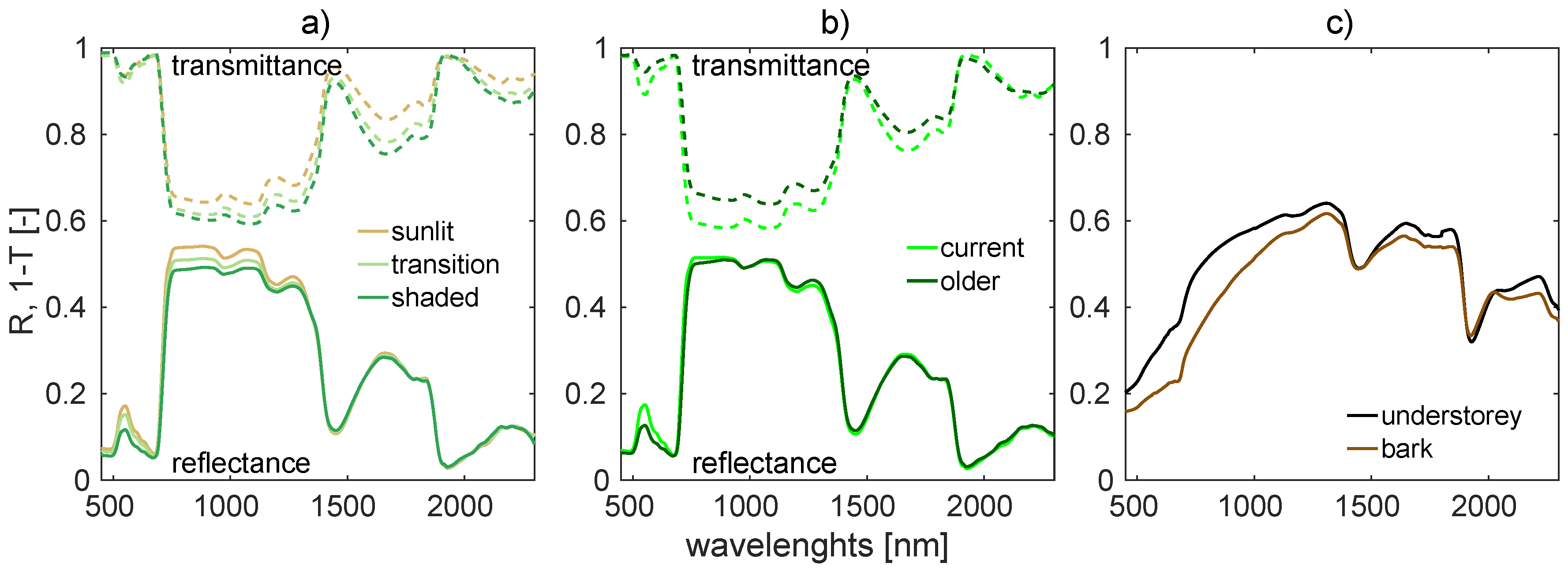
2.1.2. Needle Optical Properties
2.1.3. Remote Sensing Data
2.2. Reconstruction of 3D Spruce Tree Representation
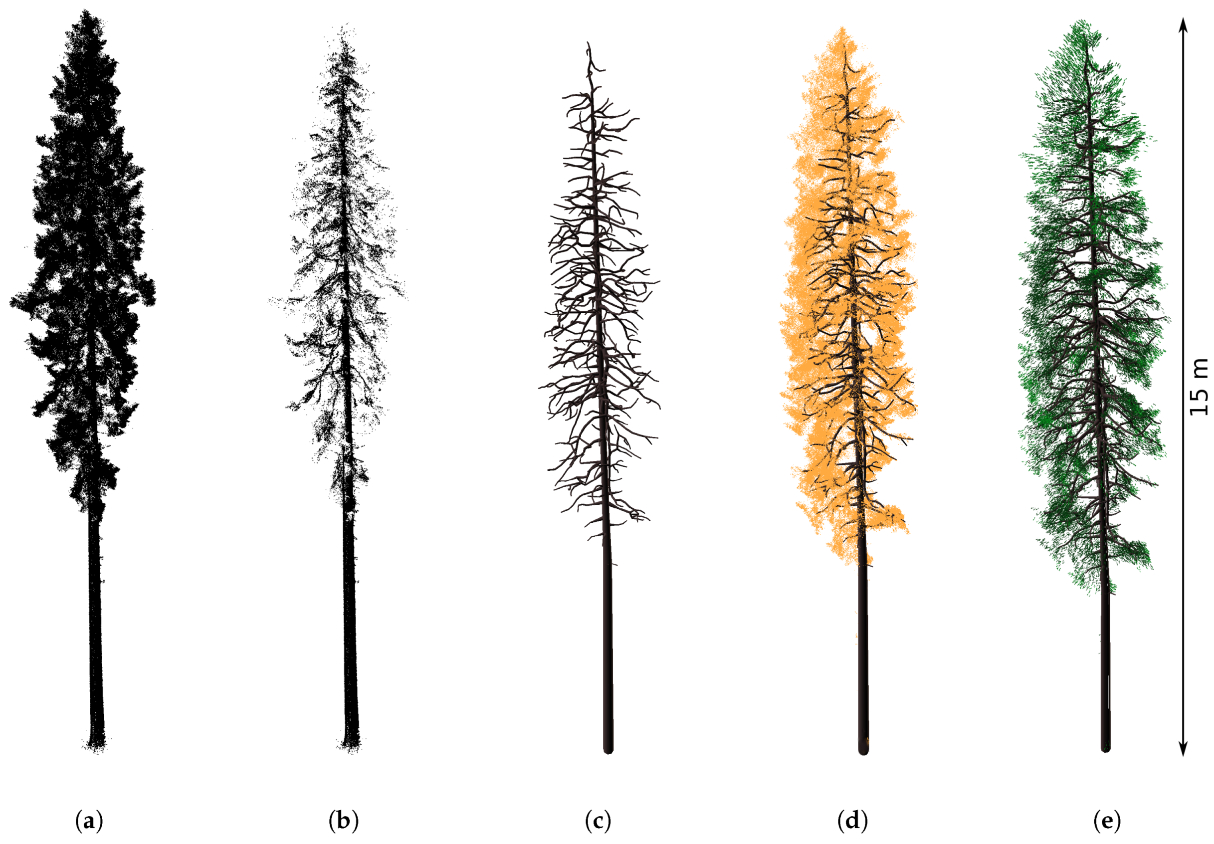
- Spatial separation and reconstruction of the wooden skeleton including trunk and main branches using an automated algorithm developed by Sloup [41] (Section 2.2.1, Figure 3b,c).
- Translation and scaling of the foliage point cloud and the reconstructed wooden skeleton to fit site-specific tree dimensions. As the TLS data had been acquired at the Černá hora site for taller trees, a scaling of dimensions was required to fit tree sizes at our Bílý Kříž primary research site (Section 2.2.2, Figure 3d).
- Distribution of shoots within the tree crown by combining the information about foliage density from the TLS data with the ancillary information on shoot angular distribution [54,55]. (Section 2.2.3, Figure 3e).
2.2.1. Reconstruction of Wooden Skeleton—Trunk and Main Branches
- Component identification: spatially related clusters of TLS points are identified and separated.
- –
- constructing a neighbourhood graph to connect close points [61];
- –
- the result is a set of components, each consisting of spatially related points belonging to the same branch or trunk part.
- Component analysis: branch-like structures are reconstructed for each identified component.
- –
- constructing a geodesic graph for each component that describes how the distance from the designated source point gradually increases throughout the component [61];
- –
- collapsing points with similar distance from the source point, unless they belong to a different sub-branch.
- Component connection: components are interconnected to form final trunk–branch structures.
- –
- initial estimation of a trunk by fitting a segmented conical model to automatically selected trunk components;
- –
- iterative selection of components to be connected to any other component while minimizing a cost function (combining the euclidean distance of the endpoints, outgoing vectors describing directions and probabilities of branch continuations, and slope function that roughly estimated expected slope of the main branches).
2.2.2. Translation and Scaling of Foliage Point Cloud
2.2.3. Shoot Distribution within a Crown
Calculation of Shoot Position
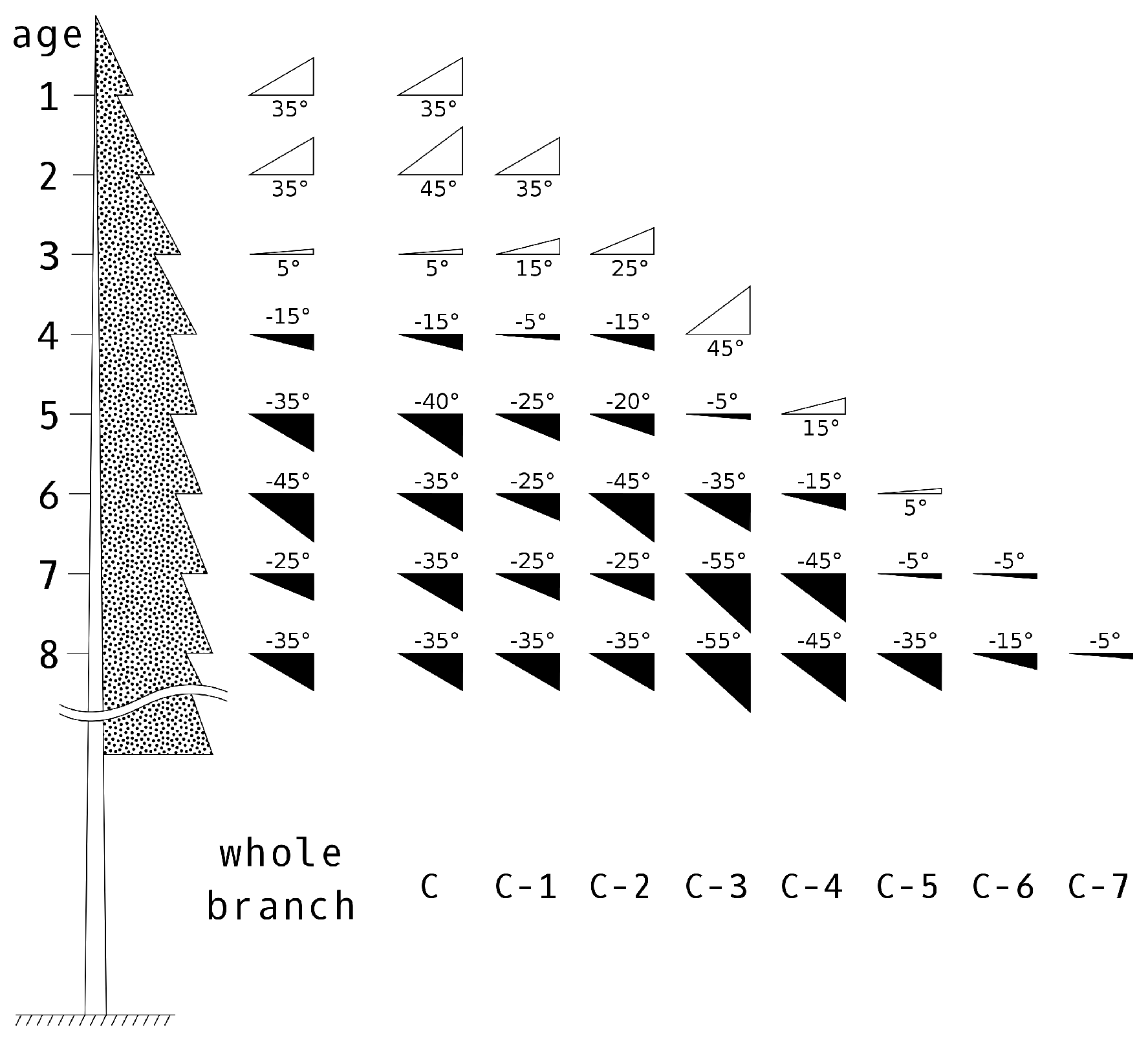
Separation of Shoots by Age Categories
Shoot Types and Their Positioning within the Crown
2.3. DART Forest Scene Parametrization
2.4. Evaluation of the Spruce Forest RT Simulations
3. Results
3.1. Reconstructed 3D Spruce Trees
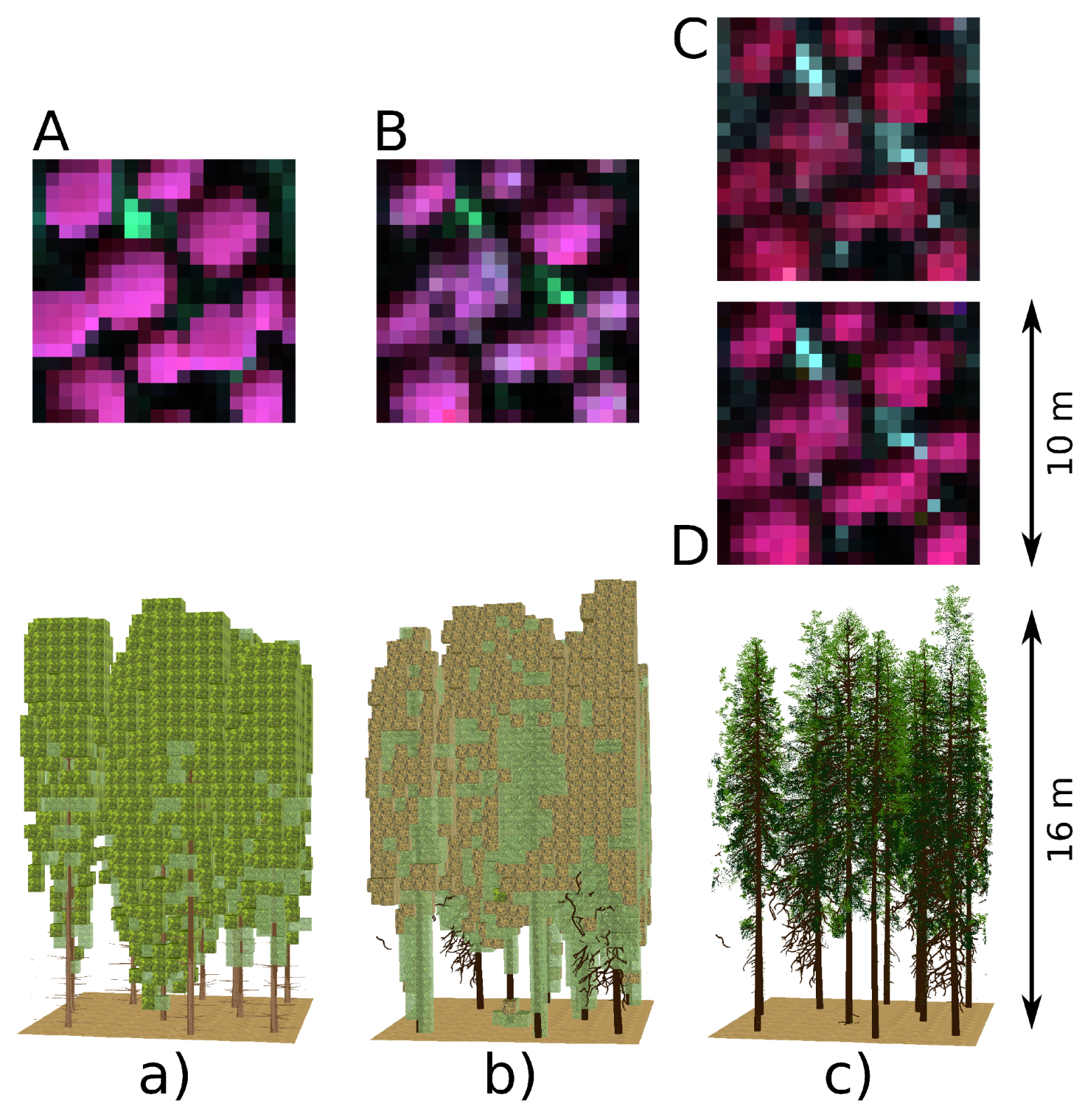
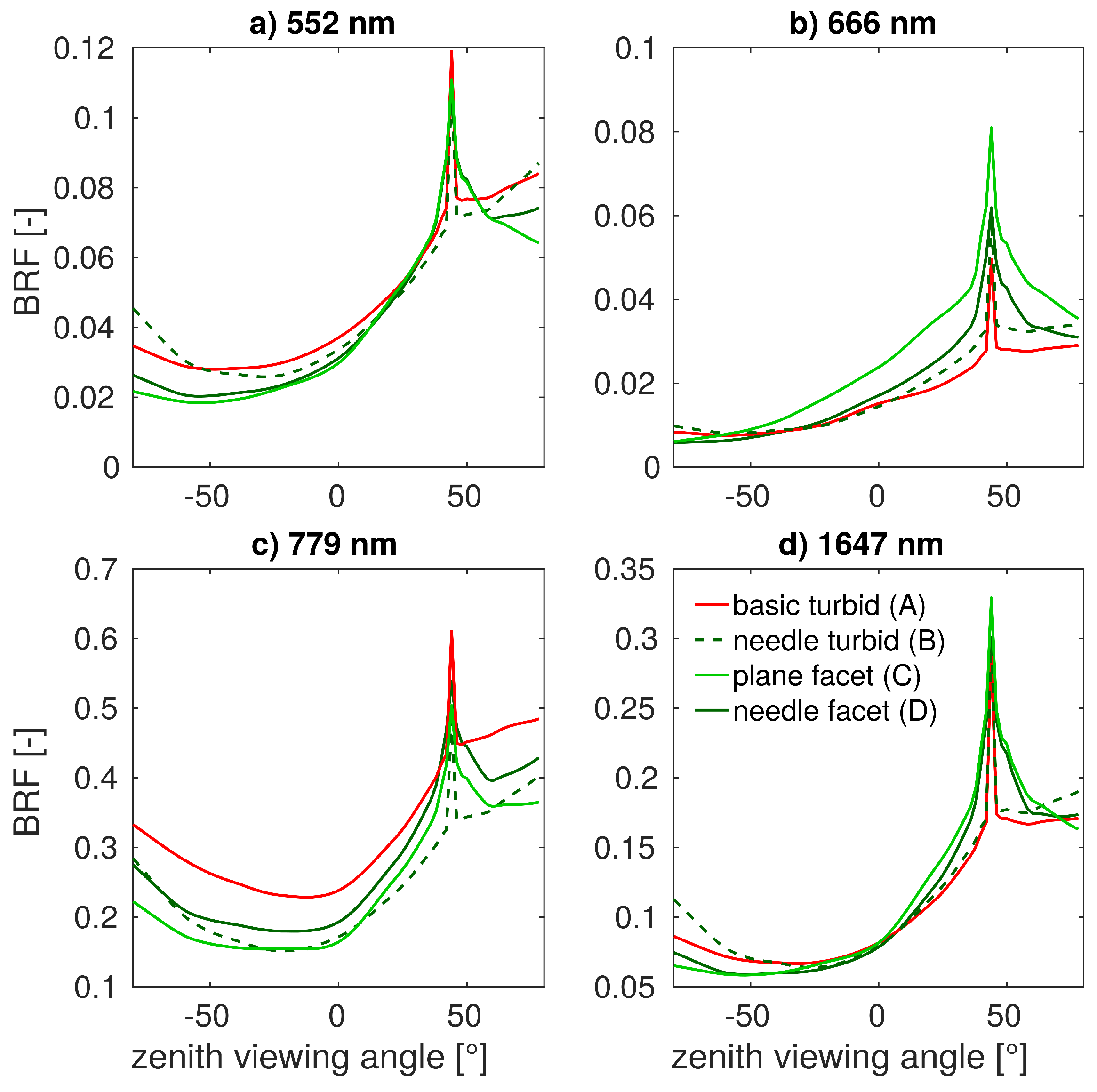
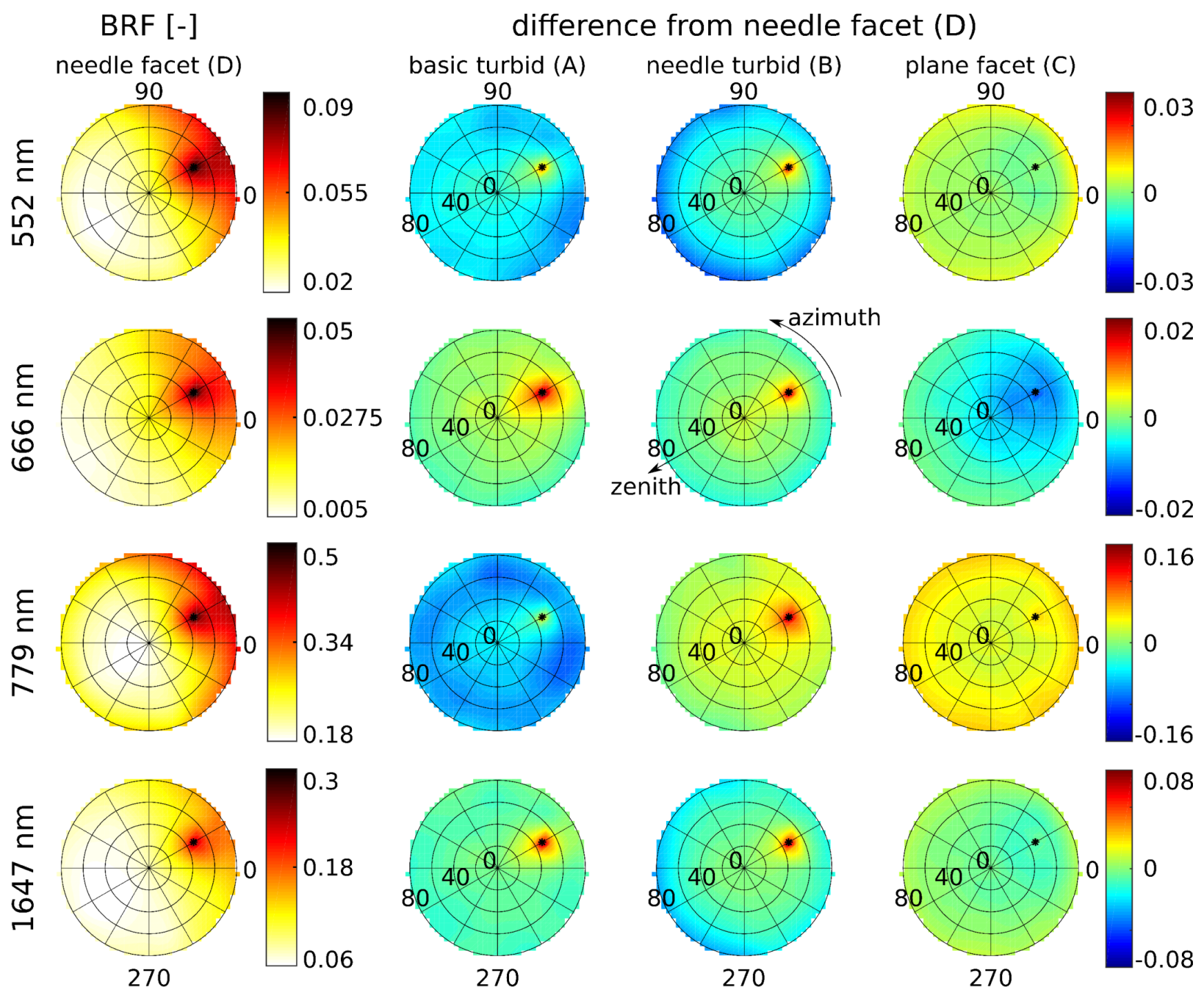
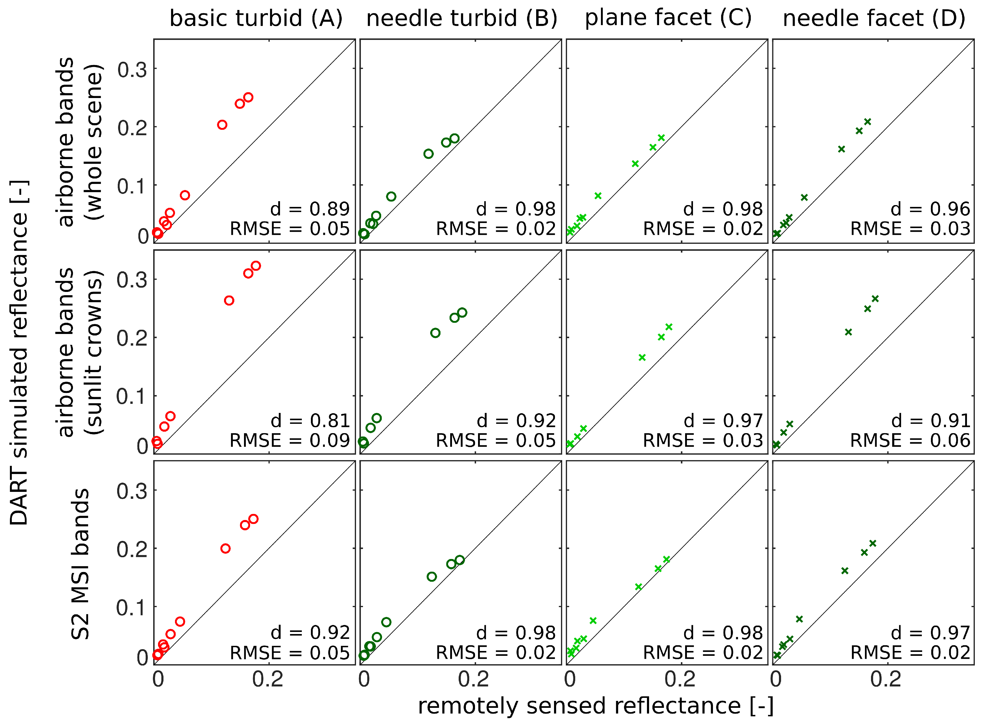
3.2. Simulations of Forest Canopy Reflectance in DART
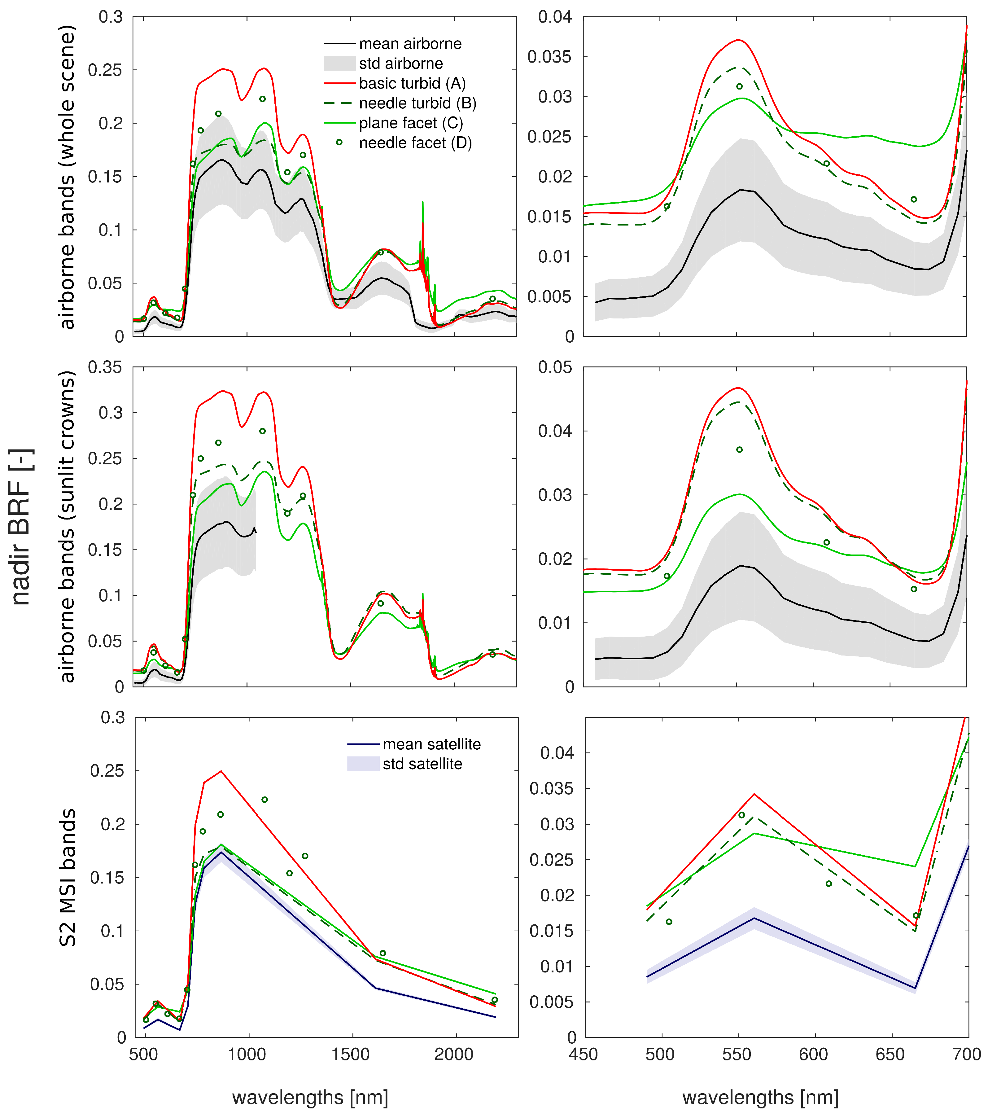
3.3. Comparison with Airborne and Satellite Data
4. Discussion
4.1. Reconstructed 3D Spruce Trees
4.2. Simulations of Forest Canopy Reflectance in DART
4.3. Comparison with Airborne and Satellite Data
5. Conclusions
Author Contributions
Funding
Acknowledgments
Conflicts of Interest
Abbreviations
| ASD | Analytical Spherical Devices |
| CASI | Compact Airborne Spectrographic Imager |
| CzeCOS | Czech Carbon Observation System |
| DART | Discrete Anisotropic Radiative Transfer |
| DBH | Diameter at Breast Height |
| FD | First Derivative |
| FLiES | Forest Light Environmental Simulator |
| FRT | Forest Radiative Transfer |
| ICOS | Integrated Carbon Observation System |
| LAD | Leaf Angle Distribution |
| LAI | Leaf Area Index |
| LiDAR | Light Detection And Ranging |
| MSI | MultiSpectral Imager |
| QSM | Quantitative Structure Model |
| RAMI | RAdiation transfer Model Intercomparison |
| RMSE | Root Mean Square Error |
| RS | Remote sensing |
| RT | Radiative Transfer |
| RTM | Radiative Transfer Model |
| SAIL | Scattering by Arbitrary Inclined Leaves |
| SASI | Smaller SWIR Airborne Spectrographic Imager |
| TLS | Terrestrial Laser Scanning |
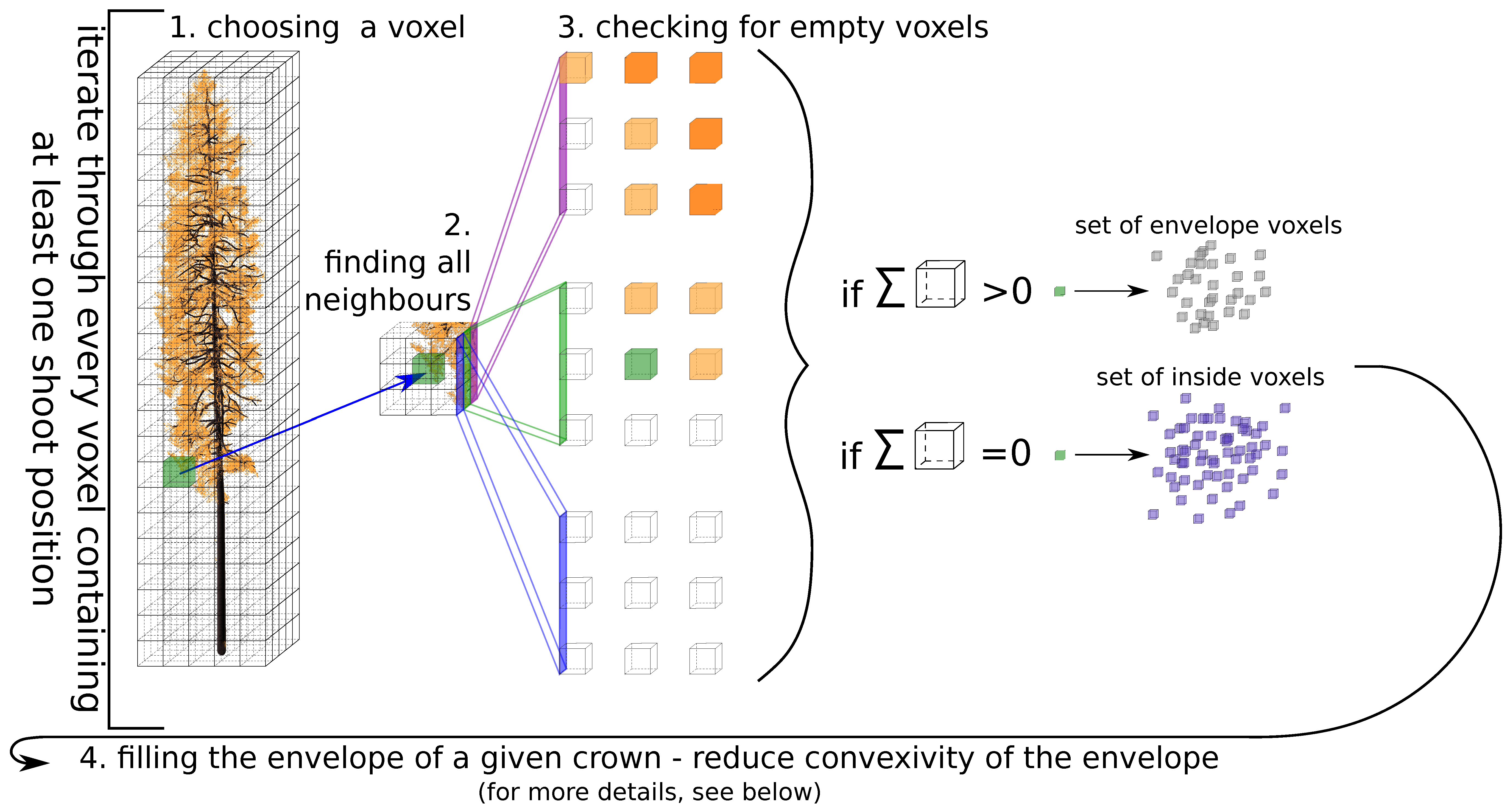
Appendix A. Finding Tree Crown Envelope
- choosing a voxel : the algorithm iterates through every voxel containing at least one shoot position;
- finding a set of all neighbours of voxel (26 voxels around the current one);
- creation of the tree envelope—checking if at least one voxel of the does not contain a shoot positions; if yes, add the to the set of edge voxels and continue with the next voxel, otherwise continue directly with the next voxel;
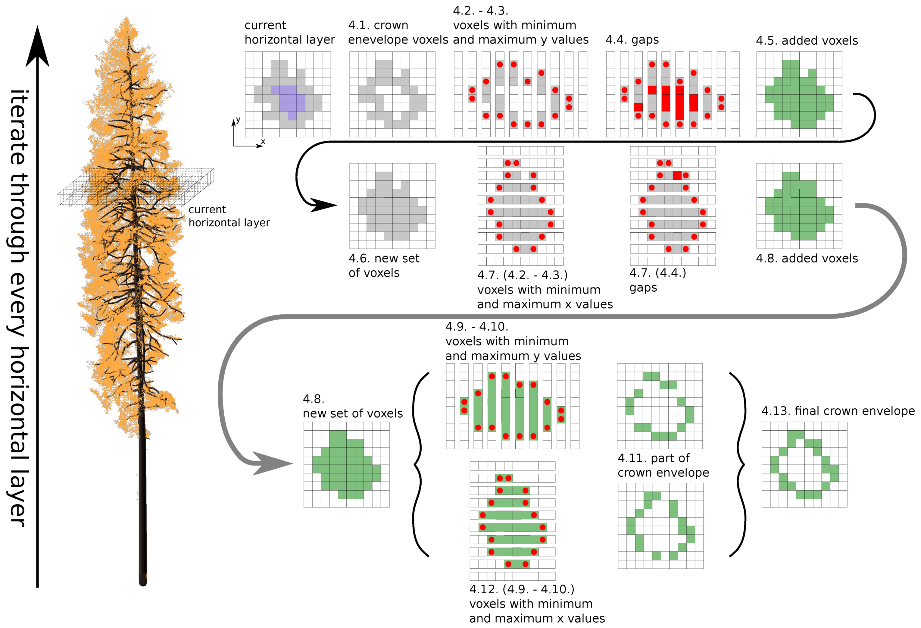
- filling the envelope of a given crown—reduce convexity of the envelope (for more details, see explanation below).

- 4.1.
- finding voxels from the crown envelope in the current horizontal layer—;
- 4.2.
- separating into lines by x coordinate;
- 4.3.
- finding cubes with minimum and maximum y coordinate values—, ;
- 4.4.
- finding gaps between and ;
- 4.5.
- if there are any gaps, fill them with new voxels;
- 4.6.
- creating a new set and adding new voxels together with voxels from ;
- 4.7.
- repeating steps 4.2.–4.5. for the y-axis;
- 4.8.
- adding new voxels into ;
- 4.9.
- separating in lines by x coordinate;
- 4.10.
- finding voxels with the minimum and maximum y coordinate values—, ;
- 4.11.
- adding voxels and into ;
- 4.12.
- repeating steps 4.9.–4.11. for the y-axis;
- 4.13.
- setting of voxels as the new set of envelope voxels for the current horizontal layer.

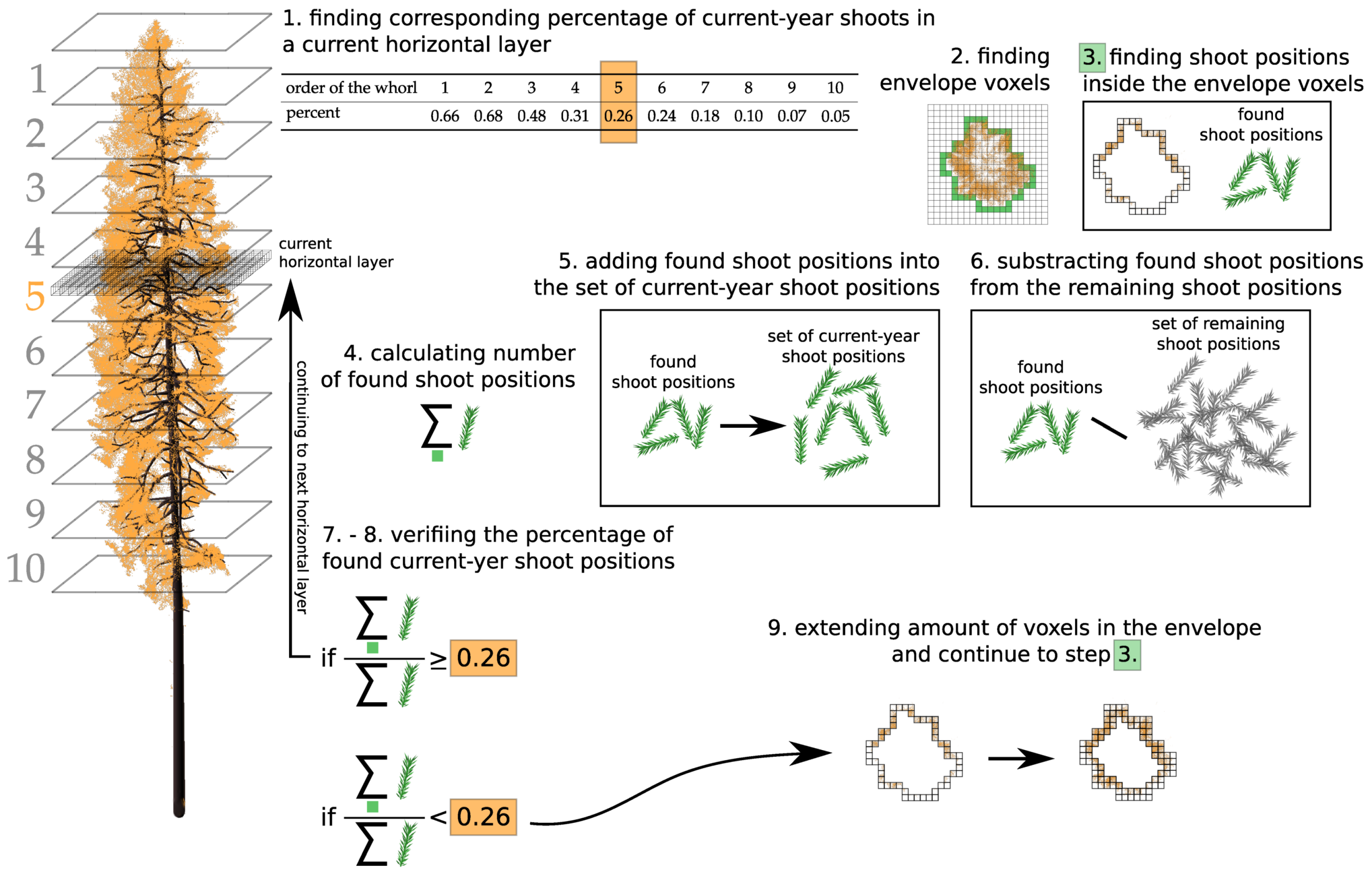
Appendix B. Assigning Shoots into Age Categories
- finding corresponding percentage of current-year shoots in a horizontal layer ;
- finding envelope voxels of the tree crown in ;
- finding shoot positions inside the envelope voxels;
- calculating number of shoot positions found;
- adding shoot positions found into the set of current-year shoot positions;
- subtracting the shoot positions found from the remaining shoot positions;
- verifying the percentage of shoot positions in the set of current-year shoot positions; testing if the percentage is higher or lower than the corresponding percentage in ;
- deciding to continue or stop the algorithm; if there are not enough current shoot positions, the algorithm continues to the next step, 9; otherwise, it continues to the next layer and repeats steps 1.–7.;
- extending amount of voxels in the envelope of tree crown towards the tree trunk in is done for x- and y-axes separately (see Figure A4);
- returning to step 3., then continuing until the end.


Appendix C. Angular Distribution of Shoots
Appendix D. Parametrization of the Basic Turbid DART Tree Representation


| Parameter | Tree 1 | Tree 2 | Tree 3 | Tree 4 |
|---|---|---|---|---|
| (1) trunk height below crown (m) | 1.55 | 4.6 | 0 | 2.5 |
| (2) trunk height within crown (m) | 13.46 | 10.41 | 16.04 | 11.5 |
| (3) trunk diameter below crown (m) | 0.26 | 0.25 | 0.27 | 0.3 |
| (4) crown height (m) | 13.45 | 10.52 | 16.26 | 11.65 |
| (5) intermediate height (m) | 9 | 10 | 9.5 | 9 |
| (6) crown projection—first axis (m) | 2.58 | 2.74 | 3.95 | 3.5 |
| (7) crown projection—second axis (m) | 2.38 | 2.88 | 3.79 | 3.3 |

| Parameter | Top | Middle | Bottom |
|---|---|---|---|
| level height relative to crown length | 0.17 | 0.3 | 0.53 |
| trunk diameter relative to one below | 0 | 0.375 | 0.75 |
| percentage of full leaf cells | 0.85 | 0.50 | 0.30 |
| start of the inner defoliation zone (a) | 0 | 0.3 | 0.75 |
| end of the inner defoliation zone (b) | 1 | 1 | 1 |
| Needle Age | |||
|---|---|---|---|
| C | C+1 | C+2 | |
| top | 0.70 | 0.20 | 0.10 |
| middle | 0.50 | 0.25 | 0.25 |
| bottom | 0.10 | 0.15 | 0.75 |
References
- Mittermeier, R.A.; Myers, N.; Thomsen, J.B.; Fonseca, G.A.B.D.; Olivieri, S. Biodiversity Hotspots and Major Tropical Wilderness Areas: Approaches to Setting Conservation Priorities. Conserv. Biol. 1998, 12, 516–520. [Google Scholar] [CrossRef]
- Myers, N. The biodiversity challenge: Expanded hot-spots analysis. Environmentalist 1990, 10, 243–256. [Google Scholar] [CrossRef] [PubMed]
- Pan, Y.; Birdsey, R.A.; Fang, J.; Houghton, R.; Kauppi, P.E.; Kurz, W.A.; Phillips, O.L.; Shvidenko, A.; Lewis, S.L.; Canadell, J.G.; et al. A Large and Persistent Carbon Sink in the World’s Forests. Science 2011, 333, 988–993. [Google Scholar] [CrossRef] [PubMed]
- Schröter, D.; Cramer, W.; Leemans, R.; Prentice, I.C.; Araújo, M.B.; Arnell, N.W.; Bondeau, A.; Bugmann, H.; Carter, T.R.; Gracia, C.A.; et al. Ecosystem Service Supply and Vulnerability to Global Change in Europe. Science 2005, 310, 1333–1337. [Google Scholar] [CrossRef] [PubMed]
- Chazdon, R.L. Beyond Deforestation: Restoring Forests and Ecosystem Services on Degraded Lands. Science 2008, 320, 1458–1460. [Google Scholar] [CrossRef] [PubMed]
- Leuning, R.; Kelliher, F.M.; Pury, D.G.G.D.; Schulze, E.D. Leaf nitrogen, photosynthesis, conductance and transpiration: Scaling from leaves to canopies. Plant Cell Environ. 1995, 18, 1183–1200. [Google Scholar] [CrossRef]
- Trumbore, S.; Brando, P.; Hartmann, H. Forest health and global change. Science 2015, 349, 814–818. [Google Scholar] [CrossRef] [PubMed]
- Chambers, J.Q.; Asner, G.P.; Morton, D.C.; Anderson, L.O.; Saatchi, S.S.; Espírito-Santo, F.D.B.; Palace, M.; Souza, C. Regional ecosystem structure and function: Ecological insights from remote sensing of tropical forests. Trends Ecol. Evol. 2007, 22, 414–423. [Google Scholar] [CrossRef] [PubMed]
- Fassnacht, F.E.; Latifi, H.; Stereńczak, K.; Modzelewska, A.; Lefsky, M.; Waser, L.T.; Straub, C.; Ghosh, A. Review of studies on tree species classification from remotely sensed data. Remote Sens. Environ. 2016, 186, 64–87. [Google Scholar] [CrossRef]
- Hansen, M.C.; Loveland, T.R. A review of large area monitoring of land cover change using Landsat data. Remote Sens. Environ. 2012, 122, 66–74. [Google Scholar] [CrossRef]
- Koch, B. Status and future of laser scanning, synthetic aperture radar and hyperspectral remote sensing data for forest biomass assessment. ISPRS J. Photogramm. Remote Sens. 2010, 65, 581–590. [Google Scholar] [CrossRef]
- Lausch, A.; Erasmi, S.; King, D.; Magdon, P.; Heurich, M.; Lausch, A.; Erasmi, S.; King, D.J.; Magdon, P.; Heurich, M. Understanding Forest Health with Remote Sensing-Part I—A Review of Spectral Traits, Processes and Remote-Sensing Characteristics. Remote Sens. 2016, 8, 1029. [Google Scholar] [CrossRef]
- Lausch, A.; Erasmi, S.; King, D.; Magdon, P.; Heurich, M.; Lausch, A.; Erasmi, S.; King, D.J.; Magdon, P.; Heurich, M. Understanding Forest Health with Remote Sensing-Part II—A Review of Approaches and Data Models. Remote Sens. 2017, 9, 129. [Google Scholar] [CrossRef]
- White, J.C.; Coops, N.C.; Wulder, M.A.; Vastaranta, M.; Hilker, T.; Tompalski, P. Remote Sensing Technologies for Enhancing Forest Inventories: A Review. Can. J. Remote Sens. 2016, 42, 619–641. [Google Scholar] [CrossRef]
- Disney, M.; Lewis, P.; Saich, P. 3D modelling of forest canopy structure for remote sensing simulations in the optical and microwave domains. Remote Sens. Environ. 2006, 100, 114–132. [Google Scholar] [CrossRef]
- Panferov, O.; Knyazikhin, Y.; Myneni, R.B.; Szarzynski, J.; Engwald, S.; Schnitzler, K.G.; Gravenhorst, G. The role of canopy structure in the spectral variation of transmission and absorption of solar radiation in vegetation canopies. IEEE Trans. Geosci. Remote Sens. 2001, 39, 241–253. [Google Scholar] [CrossRef]
- Widlowski, J.L.; Pinty, B.; Gobron, N.; Verstraete, M.M.; Diner, D.J.; Davis, A.B. Canopy Structure Parameters Derived from Multi-Angular Remote Sensing Data for Terrestrial Carbon Studies. Clim. Chang. 2004, 67, 403–415. [Google Scholar] [CrossRef]
- Verhoef, W. Light scattering by leaf layers with application to canopy reflectance modeling: The SAIL model. Remote Sens. Environ. 1984, 16, 125–141. [Google Scholar] [CrossRef]
- Verhoef, W.; Bach, H. Coupled soil–leaf-canopy and atmosphere radiative transfer modeling to simulate hyperspectral multi-angular surface reflectance and TOA radiance data. Remote Sens. Environ. 2007, 109, 166–182. [Google Scholar] [CrossRef]
- Gobron, N.; Pinty, B.; Verstraete, M.M.; Govaerts, Y. A semidiscrete model for the scattering of light by vegetation. J. Geophys. Res. Atmos. 1997, 102, 9431–9446. [Google Scholar] [CrossRef]
- Kallel, A. Vegetation radiative transfer modeling based on virtual flux decomposition. J. Quant. Spectrosc. Radiat. Transf. 2010, 111, 1389–1405. [Google Scholar] [CrossRef]
- North, P. Three-dimensional forest light interaction model using a Monte Carlo method. IEEE Trans. Geosci. Remote Sens. 1996, 34, 946–956. [Google Scholar] [CrossRef]
- Kuusk, A.; Nilson, T. A Directional Multispectral Forest Reflectance Model. Remote Sens. Environ. 2000, 72, 244–252. [Google Scholar] [CrossRef]
- Kobayashi, H.; Iwabuchi, H. A coupled 1-D atmosphere and 3-D canopy radiative transfer model for canopy reflectance, light environment, and photosynthesis simulation in a heterogeneous landscape. Remote Sens. Environ. 2008, 112, 173–185. [Google Scholar] [CrossRef]
- Govaerts, Y.M.; Verstraete, M.M. Raytran: A Monte Carlo ray-tracing model to compute light scattering in three-dimensional heterogeneous media. IEEE Trans. Geosci. Remote Sens. 1998, 36, 493–505. [Google Scholar] [CrossRef]
- Qin, W.; Gerstl, S.A.W. 3-D Scene Modeling of Semidesert Vegetation Cover and its Radiation Regime. Remote Sens. Environ. 2000, 74, 145–162. [Google Scholar] [CrossRef]
- Bailey, B.N.; Overby, M.; Willemsen, P.; Pardyjak, E.R.; Mahaffee, W.F.; Stoll, R. A scalable plant-resolving radiative transfer model based on optimized GPU ray tracing. Agric. For. Meteorol. 2014, 198–199, 192–208. [Google Scholar] [CrossRef]
- Gastellu-Etchegorry, J.P.; Demarez, V.; Pinel, V.; Zagolski, F. Modeling radiative transfer in heterogeneous 3-D vegetation canopies. Remote Sens. Environ. 1996, 58, 131–156. [Google Scholar] [CrossRef]
- Gastellu-Etchegorry, J.P.; Lauret, N.; Yin, T.; Landier, L.; Kallel, A.; Malenovský, Z.; Bitar, A.A.; Aval, J.; Benhmida, S.; Qi, J.; et al. DART: Recent Advances in Remote Sensing Data Modeling With Atmosphere, Polarization, and Chlorophyll Fluorescence. IEEE J. Sel. Top. Appl. Earth Obs. Remote Sens. 2017, 10, 2640–2649. [Google Scholar] [CrossRef]
- Gastellu-Etchegorry, J.P. DART User Manual. 2019. Available online: http://www.cesbio.ups-tlse.fr/dart/Public/documentation/contenu/documentation/DART_User_Manual.pdf (accessed on 25 March 2019).
- Prusinkiewicz, P.; Lindenmayer, A. The Algorithmic Beauty of Plants; The Virtual Laboratory, Springer: New York, NY, USA, 1990. [Google Scholar]
- Kurth, W.; Sloboda, B. Growth grammars simulating trees–an extension of L-systems incorporating local variables and sensitivity. Silva Fenn. 1997, 31, 285–295. [Google Scholar] [CrossRef]
- Pradal, C.; Fournier, C.; Valduriez, P.; Cohen-Boulakia, S. OpenAlea: Scientific Workflows Combining Data Analysis and Simulation. In Proceedings of the 27th International Conference on Scientific and Statistical Database Management, (SSDBM ’15), La Jolla, CA, USA, 29 June–1 July 2015; ACM: New York, NY, USA, 2015; pp. 11:1–11:6. [Google Scholar] [CrossRef]
- Widlowski, J.L.; Mio, C.; Disney, M.; Adams, J.; Andredakis, I.; Atzberger, C.; Brennan, J.; Busetto, L.; Chelle, M.; Ceccherini, G.; et al. The fourth phase of the radiative transfer model intercomparison (RAMI) exercise: Actual canopy scenarios and conformity testing. Remote Sens. Environ. 2015, 169, 418–437. [Google Scholar] [CrossRef]
- Gruber, F. Morphology of coniferous trees: Possible effects of soil acidification on the morphology of Norway spruce and silver fir. In Effects of Acid Rain on Forest Processes; Wiley-Liss: New York, NY, USA, 1994; pp. 265–324. [Google Scholar]
- Van Leeuwen, M.; Nieuwenhuis, M. Retrieval of forest structural parameters using LiDAR remote sensing. Eur. J. For. Res. 2010, 129, 749–770. [Google Scholar] [CrossRef]
- Dassot, M.; Constant, T.; Fournier, M. The use of terrestrial LiDAR technology in forest science: application fields, benefits and challenges. Ann. For. Sci. 2011, 68, 959–974. [Google Scholar] [CrossRef]
- Disney, M.I.; Boni Vicari, M.; Burt, A.; Calders, K.; Lewis, S.L.; Raumonen, P.; Wilkes, P. Weighing trees with lasers: Advances, challenges and opportunities. Interface Focus 2018, 8, 20170048. [Google Scholar] [CrossRef] [PubMed]
- Raumonen, P.; Kaasalainen, M.; Åkerblom, M.; Kaasalainen, S.; Kaartinen, H.; Vastaranta, M.; Holopainen, M.; Disney, M.; Lewis, P. Fast Automatic Precision Tree Models from Terrestrial Laser Scanner Data. Remote Sens. 2013, 5, 491–520. [Google Scholar] [CrossRef]
- Hackenberg, J.; Spiecker, H.; Calders, K.; Disney, M.; Raumonen, P. SimpleTree —An Efficient Open Source Tool to Build Tree Models from TLS Clouds. Forests 2015, 6, 4245–4294. [Google Scholar] [CrossRef]
- Sloup, P. Automatic Tree Reconstruction from Its Laser Scan. Master’s Thesis, Masaryk University Faculty of Informatics, Brno-Královo Pole-Ponava, Czechia, 2013. [Google Scholar]
- Ma, L.; Zheng, G.; Eitel, J.U.H.; Moskal, L.M.; He, W.; Huang, H. Improved Salient Feature-Based Approach for Automatically Separating Photosynthetic and Nonphotosynthetic Components Within Terrestrial Lidar Point Cloud Data of Forest Canopies. IEEE Trans. Geosci. Remote Sens. 2016, 54, 679–696. [Google Scholar] [CrossRef]
- Douglas, E.S.; Martel, J.; Li, Z.; Howe, G.; Hewawasam, K.; Marshall, R.A.; Schaaf, C.L.; Cook, T.A.; Newnham, G.J.; Strahler, A.; et al. Finding Leaves in the Forest: The Dual-Wavelength Echidna Lidar. IEEE Geosci. Remote Sens. Lett. 2015, 12, 776–780. [Google Scholar] [CrossRef]
- Zhu, X.; Skidmore, A.K.; Darvishzadeh, R.; Niemann, K.O.; Liu, J.; Shi, Y.; Wang, T. Foliar and woody materials discriminated using terrestrial LiDAR in a mixed natural forest. Int. J. Appl. Earth Obs. Geoinf. 2018, 64, 43–50. [Google Scholar] [CrossRef]
- Xie, D.; Wang, X.; Qi, J.; Chen, Y.; Mu, X.; Zhang, W.; Yan, G. Reconstruction of Single Tree with Leaves Based on Terrestrial LiDAR Point Cloud Data. Remote Sens. 2018, 10, 686. [Google Scholar] [CrossRef]
- Åkerblom, M.; Raumonen, P.; Casella, E.; Disney, M.I.; Danson, F.M.; Gaulton, R.; Schofield, L.A.; Kaasalainen, M. Non-intersecting leaf insertion algorithm for tree structure models. Interface Focus 2018, 8, 20170045. [Google Scholar] [CrossRef] [PubMed]
- Calders, K.; Origo, N.; Burt, A.; Disney, M.; Nightingale, J.; Raumonen, P.; Åkerblom, M.; Malhi, Y.; Lewis, P. Realistic Forest Stand Reconstruction from Terrestrial LiDAR for Radiative Transfer Modelling. Remote Sens. 2018, 10, 933. [Google Scholar] [CrossRef]
- Côté, J.F.; Widlowski, J.L.; Fournier, R.A.; Verstraete, M.M. The structural and radiative consistency of three-dimensional tree reconstructions from terrestrial lidar. Remote Sens. Environ. 2009, 113, 1067–1081. [Google Scholar] [CrossRef]
- Zheng, G.; Moskal, L.M. Leaf Orientation Retrieval From Terrestrial Laser Scanning (TLS) Data. IEEE Trans. Geosci. Remote Sens. 2012, 50, 3970–3979. [Google Scholar] [CrossRef]
- Bailey, B.N.; Mahaffee, W.F. Rapid measurement of the three-dimensional distribution of leaf orientation and the leaf angle probability density function using terrestrial LiDAR scanning. Remote Sens. Environ. 2017, 194, 63–76. [Google Scholar] [CrossRef]
- Krupková, L.; Marková, I.; Havránková, K.; Pokorný, R.; Urban, O.; Šigut, L.; Pavelka, M.; Cienciala, E.; Marek, M.V. Comparison of different approaches of radiation use efficiency of biomass formation estimation in Mountain Norway spruce. Trees 2017, 31, 325–337. [Google Scholar] [CrossRef]
- Urban, O.; Hrstka, M.; Zitová, M.; Holišová, P.; Šprtová, M.; Klem, K.; Calfapietra, C.; De Angelis, P.; Marek, M.V. Effect of season, needle age and elevated CO2 concentration on photosynthesis and Rubisco acclimation in Picea abies. Plant Physiol. Biochem. 2012, 58, 135–141. [Google Scholar] [CrossRef] [PubMed]
- Homolová, L.; Janoutová, R.; Lukeš, P.; Hanuš, J.; Novotný, J.; Brovkina, O.; Loayza Fernandez, R.R. In situ data supporting remote sensing estimation of spruce forest parameters at the ecosystem station Bílý Kříž. Beskydy 2017, 10, 75–86. [Google Scholar] [CrossRef]
- Barták, M. Struktura Koruny Smrku Ztepilého ve Vztahu k Produkci. Ph.D. Thesis, Kandidátská Dizertační Práce, Ústav Systematické a Ekologické Biologie, Brno, Czechia, 1992. [Google Scholar]
- Barták, M.; Dvořák, V.; Hudcová, L. Rozložení biomasy jehlic v korunové vrstvě smrkového porostu. Lesnictví-Forestry 1993, 39, 273–281. [Google Scholar]
- Mesarch, M.A.; Walter-Shea, E.A.; Asner, G.P.; Middleton, E.M.; Chan, S.S. A Revised Measurement Methodology for Conifer Needles Spectral Optical Properties: Evaluating the Influence of Gaps between Elements. Remote Sens. Environ. 1999, 68, 177–192. [Google Scholar] [CrossRef]
- Malenovský, Z.; Albrechtová, J.; Lhotáková, Z.; Zurita-Milla, R.; Clevers, J.G.P.W.; Schaepman, M.E.; Cudlín, P. Applicability of the PROSPECT model for Norway spruce needles. Int. J. Remote Sens. 2006, 27, 5315–5340. [Google Scholar] [CrossRef]
- Yáñez-Rausell, L.; Malenovský, Z.; Clevers, J.G.P.W.; Schaepman, M.E. Minimizing Measurement Uncertainties of Coniferous Needle-Leaf Optical Properties. Part II: Experimental Setup and Error Analysis. IEEE J. Sel. Top. Appl. Earth Obs. Remote Sens. 2014, 7, 406–420. [Google Scholar] [CrossRef]
- Hanuš, J.; Fabiánek, T.; Fajmon, L. Potential of Airborne Imaging Spectroscopy at Czechglobe. ISPRS 2016, XLI-B1, 15–17. [Google Scholar] [CrossRef]
- Richter, R.; Schläpfer, D. Geo-atmospheric processing of airborne imaging spectrometry data. Part 2: Atmospheric/topographic correction. Int. J. Remote Sens. 2002, 23, 2631–2649. [Google Scholar] [CrossRef]
- Verroust, A.; Lazarus, F. Extracting skeletal curves from 3D scattered data. In Proceedings of the Shape Modeling International’99, International Conference on Shape Modeling and Applications, Aizu-Wakamatsu, Japan, 1–4 March 1999; IEEE: Aizu-Wakamatsu, Japan, 1999; pp. 194–201. [Google Scholar] [CrossRef]
- Berk, A.; Conforti, P.; Kennett, R.; Perkins, T.; Hawes, F.; van den Bosch, J. MODTRAN6: A major upgrade of the MODTRAN radiative transfer code. In Proceedings of the Algorithms and Technologies for Multispectral, Hyperspectral, and Ultraspectral Imagery XX, Baltimore, MD, USA, 13 June 2014; International Society for Optics and Photonics: Bellingham, WA, USA, 2014; Volume 9088, p. 90880H. [Google Scholar] [CrossRef]
- Malenovský, Z.; Martin, E.; Homolová, L.; Gastellu-Etchegorry, J.P.; Zurita-Milla, R.; Schaepman, M.E.; Pokorný, R.; Clevers, J.G.; Cudlín, P. Influence of woody elements of a Norway spruce canopy on nadir reflectance simulated by the DART model at very high spatial resolution. Remote Sens. Environ. 2008, 112, 1–18. [Google Scholar] [CrossRef]
- Malenovský, Z.; Homolová, L.; Zurita-Milla, R.; Lukeš, P.; Kaplan, V.; Hanuš, J.; Gastellu-Etchegorry, J.P.; Schaepman, M.E. Retrieval of spruce leaf chlorophyll content from airborne image data using continuum removal and radiative transfer. Remote Sens. Environ. 2013, 131, 85–102. [Google Scholar] [CrossRef]
- Yáñez, L.; Homolová, L.; Schaepman, M.E.; Malenovský, Z. Geometrical and structural parametrization of forest canopy radiative transfer by LIDAR measurements. In Proceedings of the 21th ISPRS Congress, Beijing, China, 3–11 July 2008. [Google Scholar] [CrossRef]
- Yáñez-Rausell, L.; Malenovský, Z.; Rautiainen, M.; Clevers, J.G.P.W.; Lukeš, P.; Hanuš, J.; Schaepman, M.E. Estimation of Spruce Needle-Leaf Chlorophyll Content Based on DART and PARAS Canopy Reflectance Models. IEEE J. Sel. Top. Appl. Earth Obs. Remote Sens. 2015, 8, 1534–1544. [Google Scholar] [CrossRef]
- Stenberg, P. Simulations of the effects of shoot structure and orientation on vertical gradients in intercepted light by conifer canopies. Tree Physiol. 1996, 16, 99–108. [Google Scholar] [CrossRef]
- Smolander, S.; Stenberg, P. A method to account for shoot scale clumping in coniferous canopy reflectance models. Remote Sens. Environ. 2003, 88, 363–373. [Google Scholar] [CrossRef]
- Rautiainen, M.; Mõttus, M.; Yáñez-Rausell, L.; Homolová, L.; Malenovský, Z.; Schaepman, M.E. A note on upscaling coniferous needle spectra to shoot spectral albedo. Remote Sens. Environ. 2012, 117, 469–474. [Google Scholar] [CrossRef]
- Mõttus, M.; Rautiainen, M.; Schaepman, M.E. Shoot scattering phase function for Scots pine and its effect on canopy reflectance. Agric. For. Meteorol. 2012, 154–155, 67–74. [Google Scholar] [CrossRef]
- Pokorný, R.; Marek, M.V. Test of Accuracy of LAI Estimation by LAI-2000 under Artificially Changed Leaf to Wood Area Proportions. Biol. Plant. 2000, 43, 537–544. [Google Scholar] [CrossRef]


| Whorl Order | 1 | 2 | 3 | 4 | 5 | 6 | 7 | 8 | 9 | >10 |
|---|---|---|---|---|---|---|---|---|---|---|
| whorl hight (m) | 0–1 | 1–2 | 2–3 | 3–4 | 4–5 | 5–6 | 6–7 | 7–8 | 8–9 | >9 |
| % of current shoots | 1 | 0.82 | 0.61 | 0.49 | 0.35 | 0.29 | 0.23 | 0.17 | 0.07 | 0.05 |
| mean shoot elevation angle (°) | 35 | 35 | 5 | −15 | −35 | −45 | −25 | −35 | −32 | −35 |
| elevation angle variation (°) | 30–40 | 30–40 | 0–20 | −20–15 | −45–5 | −50–−5 | −40–−5 | −50–−20 | −50–−20 | −50–−20 |
| Parameter | Value |
|---|---|
| scene dimension | 10 m |
| cell dimension | 0.5 m |
| terrain | flat |
| number of trees | 10 |
| scene canopy cover | 80% |
| scene LAI | 8.5 |
| average tree height | 15 m |
| sun zenith angle | 44° |
| sun azimuth angle | 153° |
| Scenario Label | 3D Tree Rep. | 3D Shoot Rep. | DART Forest Scene Types |
|---|---|---|---|
| Abasic turbid | DART predefined tree crown shapes | not applicable | turbid cells |
| Bneedle turbid | reconstructed from laser scans | exact 3D needles | transformed into turbid cells |
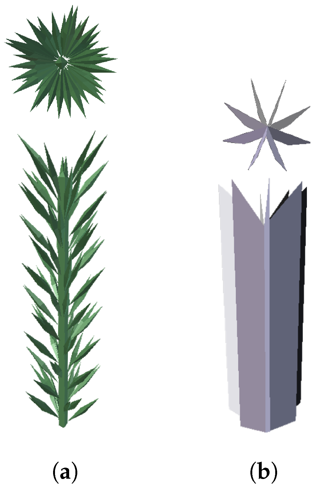
| Cplane facet | reconstructed from laser scans | simplified 3D shoots as planes | 3D shoots with object facets |
| Dneedle facet | reconstructed from laser scans | exact 3D needles | 3D needle object facets |
| Parameter | Tree 1 | Tree 2 | Tree 3 | Tree 4 |
|---|---|---|---|---|
| tree height (m) | 15.0 | 15.1 | 16.3 | 14.0 |
| crown length (m) | 13.5 | 10.5 | 13.0 | 11.5 |
| crown diameter (m) | 2.3 | 2.5 | 3.5 | 3.7 |
| number of wood facets | 112, 448 | 106, 112 | 186, 432 | 197, 760 |
| number of leaf facets | 11, 617, 576 | 16, 829, 376 | 30, 385, 824 | 30, 791, 232 |
| proportion of current shoot facets | 0.40 | 0.47 | 0.29 | 0.22 |
© 2019 by the authors. Licensee MDPI, Basel, Switzerland. This article is an open access article distributed under the terms and conditions of the Creative Commons Attribution (CC BY) license (http://creativecommons.org/licenses/by/4.0/).
Share and Cite
Janoutová, R.; Homolová, L.; Malenovský, Z.; Hanuš, J.; Lauret, N.; Gastellu-Etchegorry, J.-P. Influence of 3D Spruce Tree Representation on Accuracy of Airborne and Satellite Forest Reflectance Simulated in DART. Forests 2019, 10, 292. https://doi.org/10.3390/f10030292
Janoutová R, Homolová L, Malenovský Z, Hanuš J, Lauret N, Gastellu-Etchegorry J-P. Influence of 3D Spruce Tree Representation on Accuracy of Airborne and Satellite Forest Reflectance Simulated in DART. Forests. 2019; 10(3):292. https://doi.org/10.3390/f10030292
Chicago/Turabian StyleJanoutová, Růžena, Lucie Homolová, Zbyněk Malenovský, Jan Hanuš, Nicolas Lauret, and Jean-Philippe Gastellu-Etchegorry. 2019. "Influence of 3D Spruce Tree Representation on Accuracy of Airborne and Satellite Forest Reflectance Simulated in DART" Forests 10, no. 3: 292. https://doi.org/10.3390/f10030292
APA StyleJanoutová, R., Homolová, L., Malenovský, Z., Hanuš, J., Lauret, N., & Gastellu-Etchegorry, J.-P. (2019). Influence of 3D Spruce Tree Representation on Accuracy of Airborne and Satellite Forest Reflectance Simulated in DART. Forests, 10(3), 292. https://doi.org/10.3390/f10030292