Article

Interactive Effects of Climatic Factors on Seasonal Vegetation Dynamics in the Central Loess Plateau, China

1
School of Science, Northwest A&F University, Yangling 712100, China
2
School of Forestry, Northwest A&F University, Yangling 712100, China
3
School of Natural Resource, University of Missouri, Columbia, MO 65211, USA
4
Key Laboratory of Geographical Processes and Ecological Security in Changbai Mountains, Ministry of Education, School of Geographical Sciences, Northeast Normal University, Changchun 130024, China
*
Author to whom correspondence should be addressed.
Forests 2019, 10(12), 1071; https://doi.org/10.3390/f10121071
Submission received: 21 October 2019 / Revised: 12 November 2019 / Accepted: 18 November 2019 / Published: 25 November 2019
(This article belongs to the Section Forest Ecology and Management)

Abstract

:
The interactive effects of climatic factors (precipitation and temperature) on vegetation growth can be characterized by their effect on vegetation seasonal dynamics. The interactive effects, seasonal trend of vegetation growth, and its future consistency (potential for future trend) have not been adequately studied in the literature. In this work, using the Enhanced Vegetation Index (EVI) and gridded climate data at a resolution of 250 m in the central Loess Plateau region, we examined seasonal vegetation dynamics with climate changes and the interactive effects of climatic factors on vegetation growth at the pixel and regional scales from the period 2000 to 2015. Vegetation cover in the Central Loess Plateau in China has dramatically changed due to the Grain-for-Green (GFG) ecological restoration program, which was designed to convert cropland to forestland or grassland since 1999. Our results show that the EVI increased significantly during the 16 year period and is likely to continue to increase in the near future. Relatively small Hurst exponents for forestland suggests that the potential for a future increased trend will be weak for the forest. Large Hurst exponents for grassland indicate its strong potential of further increase. Significant increases in spring precipitation have promoted vegetation growth, while significant decreases in summer temperature have had negative effects on vegetation growth. For temperatures between 10 to 20 °C, the impact of temperature on vegetation growth has a clear positive relationship with the moderator variable precipitation. For precipitation < 200 mm in the growing season, the impact of precipitation on vegetation growth has a clearly positive relationship with the moderator variable temperature. Results of this study will provide useful and important guidelines for designing forestland and grassland restoration plans in arid, semiarid and sub-humid regions.

1. Introduction

Vegetation dynamics are strongly affected by climate changes [1,2,3,4]. Ecosystems in arid, semiarid, and semi-humid regions are usually unstable and particularly vulnerable to environmental changes, such as climate changes, desertification, and soil erosion [5,6,7]. Recently, researchers have recognized the importance of interactions between climatic factors in driving vegetation dynamics and their responses to climate changes [5,7,8]. Those interactions are particularly important for controlling seasonal vegetation dynamics as modified by biophysical, ecological and physiological processes, such as photosynthesis, disturbance, and competition [9]. Thus, understanding the interactions of climatic factors relative to vegetation dynamics has emerged as an important research task, especially for managing vegetation restoration in the aforementioned regions.
Substantial research progress has been achieved in studying vegetation dynamics under climate changes in arid, semiarid and semi-humid regions by using the satellite earth observation time-series data, for example the Normalized Difference Vegetation Index (NDVI) data [5,10,11,12]. Studies in the Tibetan Plateau region have found that vegetation cover has mainly been affected by climatic factors and increased as temperature and precipitation increased [13,14]. In central Asia, precipitation has been identified as the main factor driving vegetation growth, while temperature has been identified as a control variable for vegetation greenness [11,15,16]. The characterization and understanding of historical changes is important for understanding future trends. Predicting that future trend is challenging [17] due to complex vegetation–climate interactions [18], as well as delayed responses of vegetation growth to climate changes [19]. A few studies [11,17,20,21] have performed trend analysis using the Hurst exponent, which characterizes the autocorrelation of time series or index of long-range dependence. However, the positive or negative direction of future vegetation growth trends in different seasons has not been carefully studied using this approach.
Recent research has recognized the interactive and moderation effects of various climate factors [22,23]. For example, the study in [23] showed that the increase in summer precipitation had the strongest positive impact on NDVI slopes, and the interactions between mean annual temperature and changes in mean annual temperature had a positive relationship on NDVI slopes in the Great Yellowstone Ecosystem from 1989 to 2014. The study in [22] investigated the multifactor interactive effects of precipitation, temperature, and CO2 on the changes in carbon and water in the ecosystem. The study in [24] showed that the interactions between elevated CO2 and global warming were antagonistic on total vegetation biomass. The vegetation growth might be overestimated if only individual climate factors were used in the analysis [24]. Concurrent changes in multiple climate factors triggers complex interactive effects on vegetation growth [22,24]. In recent studies, vegetation dynamic models considering global climate changes at large scales have been developed to analyze bidirectional vegetation–climate interactions [9,25,26,27]. However, these models relied on simultaneous vegetation indicators and meteorological data, which have often involved high levels of uncertainty [19]. Data-driven approaches (e.g., neural and Granger causality analyses [28]) have been developed to study drivers of climatic behaviors. Their results show that anthropogenic activity was the major factor in temperature changes [27,28]. The study in [28] examined the interaction between vegetation and climate changes in the Loess Plateau region of China using the Granger causality. It showed that there were indeed interactions between local climate and vegetation changes. However, specific interactive effects between climatic factors and vegetation growth have not been carefully examined.
In this work, we focused on studying the interactive effects of climatic factors on vegetation dynamics. We proposed the use of simple-slope analysis [29,30] and the Johnson-Neyman technique [31] to perform in-depth analysis of the interactive effects between vegetation growth and major climate factors, such as precipitation and temperature. We hypothesized that the interactive effects of climatic factors would affect vegetation growth seasonally, and it could provide a better understanding of the climate changes on vegetation growth. These two methods have been successfully used in psychology studies [32,33] and medical applications [34] to analyze dependency and interactive effects between different study variables. However, they have not been used for studying vegetation–climate relationships, especially for different seasons. Compared to nonlinear methods, the simple-slope analysis and Johnson-Neyman technique have the advantage of being able to more directly and robustly capture the detailed interactions of climatic factors on vegetation growth [17,18,35]. Another important factor to be considered is global climate change. In this case, the interaction models between climatic factors on vegetation growth should be adapted. For example, in some areas global warming may cause an increase in precipitation and soil moisture.
With arid, semi-arid and sub-humid climates, the Loess Plateau region has experienced severe soil erosion for decades [36,37,38]. Grain-for-Green (GFG), one of the world’s largest ecological restoration projects, was launched in 1999 on the Loess Plateau by the Chinese government to convert inappropriate croplands to forests or grasslands. As a result, vegetation coverage has considerably increased. For example, the NDVI had an increased rate of 0.0015 per year over the entire Plateau from 1981 to 2010 [7,36,37,38]. Although the GFG has achieved great progress, researchers have found some negative consequences, such as poor plantation sustainability, decreased soil moisture, death of natural vegetation with shallow roots [39,40,41].
This study aimed to analyze seasonal vegetation dynamics, including observed and future trends, in relation to climate changes, as well as the interactions of climate factors in relation to vegetation changes in the central Loess Plateau region. Precipitation and temperature are the dominant climatic factors affecting vegetation growth [11,19]. Therefore, we focused on these two climate factors. Specific objectives of this study were to (1) investigate seasonal observed vegetation growth and its consistency in response to climate change in the central Loess Plateau region during the periods of 2000 to 2015; (2) study the impacts of climate factors on vegetation growth; and (3) analyze the interactive effects of climate factors (precipitation and temperature) on vegetation growth.
We chose the enhanced vegetation index (EVI) data in MOD13Q1 products because EVI sensitively captures the seasonal vegetation variation compared to the NDVI [42,43]. The seasons studied were the growing season (April–September), spring (March–May), summer (June–August), autumn (September–November), and winter (December–January). Note that only the inter-annual variation analysis included winter. Other analyses mainly focused on the growing season, spring, summer, and autumn because of little vegetation greenness in winter.

2. Materials and Methods

2.1. Study Area

Our study area, a key experimental area of the GFG project, was the central Loess Plateau (Yanan) in China, covering 3.7 million hectares (Figure 1a; 35°21′ N–37°31′ N, and 107°41′ E–110°31′ E). It is a typical loess hilly region, experiencing severe soil erosion. Forestland of the study region was mainly distributed in the south and grassland was mainly in the north (Figure 1b). Cropland was scattered in the study area (Figure 1b). The climate was inland arid, semiarid, and semi-humid with four distinct seasons, abundant sunshine, and a large diurnal temperature difference. The average annual temperature was 6.3–13.7 °C (Figure 1c), decreasing from the Southeast to Northwest, while the total average precipitation was 443.9–707.2 mm (Figure 1d), increasing from north to south with large seasonal and annual variations. The elevation range was 392–1804 m.
Vegetation cover varied greatly within the study area. We calculated the average annual EVI of the growing season at the pixel level for 2000–2015 (Figure 1a). Average EVI in the growing season was large in the south and small in the north. The statistical classification (Figure 1a) of average EVI showed that the area with low EVI values (0.1–0.2) was mainly in the north and accounted for 50.3% of the study area. Areas with EVI values between 0.2 and 0.3 were mainly in the southeast and southwest, about 36.9% of the study area. Areas with large EVI values (0.3–0.4) were in the mid-south, accounting for 12.3% of the study area. The area with EVI values <0.1 or >0.4 was relatively small (0.45%).

2.2. Data Sources

The Enhanced Vegetation Index (EVI) is designed to enhance the vegetation signal by a reduction in the canopy background signal and atmosphere influence. EVI is defined as
E V I = G N I R R e d N I R + C 1 R e d C 2 B l u e + L ,
where NIR, Red, and Blue are the full or partially atmospheric-corrected surface reflectance; L is the canopy background adjustment; C1 and C2 are the coefficients of the aerosol resistance term; and G is a scaling factor. The coefficients were L = 1, C1 = 6, C2 = 7.5, and G = 2.5 adopted for the MODIS-EVI algorithm.
We used time-series EVI data of 2000–2015 from the Terra sensor MOD13Q1 product with a spatial resolution of 0.017° (approximately 250 m). The images were geometrically and atmospherically corrected [44]. The dataset had 16-day intervals over periods of 16 years. Twenty-three EVI images were obtained for each year using the maximum value composite (MVC) method. These included quality assessment files used to mask out pixels for cloud, shade, water, snow or areas with high aerosol contents [8,45]. From the moderate Resolution Imaging Spectroradiometer (MODIS) data, it has been observed that clouds form and aggregate in the middle latitudes, 60 degrees north and south of the equator [46]. While at 15 and 30 degrees north, clouds are rare [46]. Our study area lay in the latitude range of 35°21′ N–37°31′ N. Thus, the MODIS data used in this study was relatively reliable for vegetation growth analysis. For each year, we obtained monthly EVI data using the MVC approach [1]. Mean EVI was also calculated for each year, the growing season, spring, summer, and autumn. Pixels with average monthly and seasonal EVI values not greater than zero were treated as non-vegetation areas and were excluded to reduce the effects of clouds, water and snow cover [1].
We obtained daily mean precipitation and temperature data from 839 meteorological stations over the time period 2000 to 2015 from the China Meteorological Data Sharing Service System (http://cdc.cma.gov.cn). We used the ANUSPLIN 4.3 algorithm, which was based on the thin-plate spline function, to interpolate the meteorological data [47]. This method can greatly improve precision by incorporating major impact factors as covariates into the interpolation process. In our study, latitude, longitude, and monthly temperature or precipitation of each meteorological station were used as independent variables and elevation as a covariate in the interpolation process [47]. Elevation data was obtained from the digital elevation model (DEM) from the National Imagery and Mapping Agency (NIMA) Shuttle Radar Topography Mission (SRTM) of NASA (http://glcf.umd.edu/data/srtm/). The daily climate data were converted to monthly average and interpolated to grids at resolution of 0.1°. Precipitation and temperature datasets were extracted from the boundary vector file of the study area using the batch method in ArcMap Version 10.5 software (Esri Inc, Redlands, CA, USA). Precipitation and temperature datasets were resampled from 0.1° to 0.017° using mask analysis in ArcMap 10.5 for the harmonization of datasets and further correlation analysis with the EVI [47]. Average precipitation and temperature for the growing season (April–September), spring (March–May), summer (June–August), autumn (September–November), and winter (December–January) were also calculated for subsequent analyses.

2.3. Data Analysis

2.3.1. Observed Trend Analysis of Enhanced Vegetation Index and Climatic Factors

Two methods were used in this work for trend analysis: the ordinary least squares (OLS) method [1] and Theil–Sen trend analysis [48]. We used OLS to study the relationship between observed interannual variations of the seasonal EVI and climatic factors at the regional scale from 2000–2015 (Figure 2). The significance of those variations was tested at the 0.05 level. The OLS slope was calculated as:
S = n × i = 1 n i × E V I i i = 1 n i i = 1 n E V I i n × i = 1 n i 2 ( i = 1 n i ) 2 ,
where n represents the total number of years; year i ranges from 1 to 16 and EVIi is the average maximum EVI in i. We also used the Theil–Sen trend analysis, a robust nonparametric statistical method [3,20], to investigate observed trends of EVI and climatic factors at the pixel level from 2000–2015 (Figure 3). The Theil–Sen median SEVI was calculated as:
S E V I = m e d i a n   ( E V I j E V I i j i ) ,     1 i < j 16 ,
where EVIi and EVIj are the EVI values in years i and j, respectively. If SEVI is > 0, the EVI has an upward trend; otherwise, it has a downward trend. The Mann–Kendall trend test [49] was used to test the significance of the observed trend of EVI and climate factors from 2000 to 2015. This test, based on a nonparametric statistical method, had two major advantages: (1) it did not require samples to follow certain distributions, and (2) it was not sensitive to outliers [20]. The test statistics were calculated using:
Z = { S 1 v a r ( S ) S > 0 0 S = 0 S + 1 v a r ( S ) S < 0 ,
where S = j = 1 n 1 i = j + 1 n s g n   ( E V I j E V I i ) ; v a r ( S ) = n ( n 1 ) ( 2 n + 5 ) 18 ; and sgn is the sign function. For the two-sides hypothesis test, | Z | > u α / 2 indicates that the time-series trend is significant. We chose a significance level of α = 0.05. The observed trend analysis and test were performed in the R environment (version 3.4.4) using the trend package.

2.3.2. Consistency of Vegetation Growth Trend

We used the Hurst exponent method [50] to investigate seasonal consistency of the vegetation growth trend at the pixel level over 2000–2015 in the study area. The Hurst exponent (H) [20] is a statistical measurement used to characterize the consistency of time series, and has been widely used in climatological, ecological, and geological studies. According to previous studies [11,17,20,21], the value of H ranges from 0 to 1. H = 0.5 indicates that the EVI time series is random without consistency, which means that the trend of future time series is not related to the observed trend. H > 0.5 indicates that the EVI time series have consistency, meaning that the time series trend will continue in the future. Larger values imply greater consistency. H < 0.5 represents anti-consistency of the EVI time series, which indicates an opposite trend of that series in the future, with a smaller value of H indicating greater anti-consistency.
The results of the Theil–Sen median method and the Mann–Kendall trend test were reclassified with the results of Hurst exponent analysis (Figure 4e–h) to synthesize variations in future trends for the growing season, spring, summer, and autumn (Figure 4a–d). We designated six categories (Table 1) as follows: (1) consistency and significant increase; (2) consistency and slight increase; (3) consistency and stability; (4) consistency and slight degradation; (5) consistency and severe degradation and (6) undetermined future trend.
The significant difference in the distribution of Hurst exponents between land-cover classes was tested using one-way simple ANOVA analysis for the growing season, spring, summer, and autumn. We compared different land cover types, including forest and crop, forest and grassland, and crop and grassland, respectively. We performed the ANOVA analysis in the R Version 3.4.4 environment (by R Core Team, Vienna, Austria).

2.3.3. Responses of Vegetation Growth to Climate Change

• Correlation and partial correlation analysis between EVI and climatic factors
We analyzed the responses of EVI to climate changes using Pearson correlation and partial correlation methods over 2000 to 2015. We calculated the Pearson correlation coefficient, the partial correlation coefficient between EVI and precipitation and EVI and temperature, and corresponding p-values for various months at the regional scale (Figure 5). The partial correlation coefficient between the EVI and climatic factors (precipitation and temperature) was defined as:
R x y . z = R x y R x z R y z ( 1 R x z 2 ) ( 1 R y z 2 ) ,
where Rxy.z is the partial correlation coefficient between variables x and y when z is constant. Rxy, Rxz, and Ryz represent the simple correlation coefficients between variables x and y, y and z, and x and z, respectively. We also calculated the Pearson correlation coefficient between EVI and climatic factors and the corresponding p-values for different seasons at the pixel level, in order to investigate the spatial variation of EVI responses to climate changes. The correlation results were synthesized for information on spatial correlation variation in the various seasons, which had four classes (i.e., significant positive, non-significant positive, significant negative and non-significant negative correlation). Correlations were computed in the R environment (version 3.4.4) using the packages stats and ppcor.
• Interactive effects of precipitation and temperature on vegetation growth
We used the simple-slope analysis and Johnson-Neyman method to investigate the interactive effects of precipitation and temperature on vegetation growth. In statistics and regression analysis, moderation is used when the relationship between two variables depends on a third variable. The third variable is referred to as the moderator. For example, considering the following multiple regression equation:
y = b 0 + b 1 x + b 2 z + b 3 x z + ε ,
We can rearrange the aforementioned formula as:
y = ( b 0 + b 2 z ) + ( b 1 + b 3 z ) x + ε ,
where b0, b1, b2, and b3 are the regression coefficients; ε is random error. Here, x is a focal predictor, z is a moderator.
The simple-slope analysis was analyzed using the pick-a-point approach [51]. In this method, a subset of values of interest was selected for the moderator variable. For each value, we studied the effect of the focal predictor on the analysis outcome [29,52]. Generally, the moderator is shifted by adding and subtracting one standard deviation (SD) from each observation. After this data is pre-processed, the least squares model with an interaction term is used to obtain coefficients and p-values for the focal predictor at these selected moderator values. We chose precipitation as the moderator variable and temperature as the focal predictor for the growing season, spring, summer and autumn, and vice versa. Coefficients and p-values for the effects of the focal predictor on EVI were estimated at these selected values of the moderator variable. We used both raw and mean-centered data to complete the simple slope analysis. Multiple co-linearity could have existed in these variables, and it could have been reduced using the mean-centered data. However, we found that both results were quite similar to each other (Figures S1 and S2 and Figure 6 and Figure 7). Therefore, we chose to use the raw data.
We used the Johnson-Neyman method to estimate the range of the moderator in which the focal predictor had a significant association with the outcome (EVI) [53,54]. This method extends the simple-slope analysis. It detects interactions of the focal predictor on the outcome across all observed values of the moderator in the data, not just at the selected levels of the moderator. The interactions of the focal predictor on the outcome were characterized by the direction and significance of these simple slopes [29]. The simple-slope analysis and Johnson-Neyman method were implemented with R (version 3.4.4) using the package jtools.
We tested the significant differences of EVI values at the selected moderator levels (mean + SD, mean, and mean – SD) using a one-way ANOVA analysis. The significant differences of EVI values between the selected moderator levels were also tested using one-way simple ANOVA. We compared the following three different scenarios based the selected moderator level: (1) mean + SD and mean, (2) mean + SD and mean − SD, and (3) mean and mean − SD. The ANOVA analyses were performed in the R environment (version 3.4.4).

3. Results

3.1. Observed Vegetation and Climatic Factor Dynamics

3.1.1. Temporal Variation of EVI and Climatic Factors

During the study period (2000–2015), the EVI had a strong positive linear trend with rates of 0.008, 0.006, 0.009, 0.004 and 0.002 per year for the growing season, spring, summer, autumn and winter, respectively (Figure 2). The determination coefficients (R2) were large, suggesting that the EVI time series data were well fit by the linear model.
The growing season precipitation showed an upward trend at a rate of 1.76 mm/year (Figure 2). Spring precipitation showed a strong and significant increasing trend with a rate of 1.44 mm/year (Figure 2). Summer and autumn precipitation displayed non-significant increasing trends. Winter precipitation had a non-significant decreasing trend. These results indicated a wetter trend in all seasons except winter during recent decades on the central Loess Plateau. Compared to precipitation, temperature exhibited a more stable trend (Figure 2). Growing season and summer temperatures showed significant decreasing trends at rates of −0.062 and −0.073 °C/year, respectively; other seasons’ temperature trends were not significant.

3.1.2. Spatial Variation of EVI and Climatic Factors

The spatial distribution of EVI showed a significant increasing trend for most areas in all seasons during 2000–2015 (Figure 3a–d). However, EVI slope values had greater spatial heterogeneity across seasons. Growing season and summer had relatively large values, and areas with steep EVI slopes (≥0.01) were mainly in the north and east. Spring and especially autumn had relatively small EVI slope values in most areas.
Growing season and summer temperatures showed a significant decrease for most areas, accounting for 61.9% and 64.4% of the study area, respectively. Areas with large slope values were in the north and center (Figure 3i–m). Spring temperature had a non-significant decreasing trend in most areas, whereas autumn temperature had an upward trend in most areas.

3.2. Seasonal Consistency of Vegetation Dynamics

We examined the future trend of EVI for all six classes (Figure 4a–d) by reclassifying the results of the spatial trend using Hurst exponent analyses (Figure 4e–h). The future trend of EVI showed a wide distribution of consistency. The areas of increase were 96.1%, 87.3%, 92% and 76.7% of the total area for growing season, spring, summer, and autumn, respectively (Figure 4a–d).
The average Hurst exponent was 0.65, 0.62, 0.64 and 0.63 for the growing season, spring, summer, and autumn, respectively. The difference in Hurst exponents between land cover classes was significant for all the compared land cover classes in all seasons (p-value < 0.001) (Table 2). The forest had the smallest average Hurst exponents compared to grassland and crop (Table 3). However, the spatial distribution of the Hurst exponent had large seasonal variations (Figure 4e–h). In the growing season, the area with large Hurst exponents (0.7–0.75) was in the Northwest of the study area (8.6%), and the area with Hurst exponents 0.65–0.7 and 0.5–0.6 accounted for 53% and 30.4% of the study area, respectively.
In spring, the area with large Hurst exponents (0.7–0.75) was relatively small. The area with exponents 0.65–0.7 was mainly in the Northwest, accounting for 28.7% of the total area. Small exponents (<0.6) were found mainly in the center, south, and east, about 30% of the total area. The distribution of the summer Hurst exponent was very similar to that in the growing season, and the autumn distribution was similar to that in spring.

3.3. Responses of Vegetation Growth to Climate Change

3.3.1. Monthly Correlation Variation of EVI and Climate Factors

Correlation coefficients between EVI and precipitation and EVI and temperature both showed large monthly variations (Figure 5). EVI and precipitation had a positive correlation from February through November (except in June with a negative partial correlation coefficient) (Figure 5a). The correlation coefficients between EVI and precipitation during February through May were obviously greater than those from June through November, and the peak occurred in April. EVI and precipitation had a significant negative correlation in January and a strong negative correlation in December.
The correlation between EVI and temperature was positive in most months from January through April, and the partial correlation was significant and positive in April (Figure 5b). However, the value changed dramatically from positive to negative during April (0.25 and 0.52 for correlation and partial correlation coefficients respectively) to May (−0.36 and −0.34 for correlation and partial correlation coefficients, respectively). The negative correlation between EVI and temperature gradually increased from May through July, and the peak was in July (−0.57 and −0.63 for correlation and partial correlation coefficients, respectively). The correlation between EVI and temperature was not significant from August through December.

3.3.2. Spatial Distribution of Correlation between Vegetation and Climate Factors

The EVI had a positive correlation with precipitation at most pixels in all seasons (56.4% of the total area in the growing season, 98.3% in spring, 95.6% in summer, and 64.3% in autumn) (Figure S3a–d, Figure 8a–d). During spring, the area with significant correlation between EVI and precipitation accounted for 63.0% of the study area and was mostly in the Northeast and west (Figure S3b, Figure 8b).
The spatial distribution of correlation coefficients between EVI and temperature showed large seasonal variations (Figure S3e–h, Figure 8e–h). The EVI had a non-significant negative correlation with temperature in most areas during the growing season and spring (Figure S3e–f, Figure 8e–f). Particularly in summer, EVI had a negative correlation with temperature in most areas (97.8%), and the area with significant negative correlation, representing 37.5% of the total area, was found in the north and some southern zones (Figure S3g, Figure 8g). The correlation between EVI and temperature was positive and non-significant in most areas during autumn (Figure S3h, Figure 8h).

3.3.3. Predicting Interactive Effects of Vegetation Growth between Climatic Factors

• Predicting interactive effects of vegetation growth with precipitation as a moderator
We used the monthly average for the whole region from 2000 to 2015 to investigate the interactive effects of climatic factors on vegetation growth. Simple slopes of temperature with vegetation growth were significant and positive in the growing season (Figure 6a). According to the Johnson-Neyman interval analysis, the simple slopes were significant and nonzero for precipitation <152 mm (observed precipitation was 8.28–209.30 mm). When precipitation was used as the moderator variable, it had an obvious positive effect of temperature on vegetation growth during the growing season for temperatures < 20 °C.
In spring, the simple slopes of temperature versus vegetation growth were significantly positive (Figure 6b). According to the Johnson-Neyman interval analysis, the simple slopes of temperature were significant and nonzero for all observed values of precipitation (which were 1.51 to 72.82 mm). The precipitation, as the moderator, played an obvious positive effect of temperature on vegetation growth for temperatures > 10 °C in spring.
In summer, the simple slopes were not significant for the three levels of precipitation (Figure 6c). In autumn, the simple slopes of temperature were significant and positive (Figure 6d). According to the Johnson-Neyman interval analysis, the simple slopes of temperature were significant and nonzero for all observed values of precipitation (which were 0.21 to 209.3 mm). The trend of simple slopes in autumn was similar to that in spring.
Since the simple slopes were obtained with the statistical fitting of data grouped by the selected moderator levels, the significant differences of EVI values at the selected moderator levels were tested using the one-way ANOVA analysis (Table 4). The significant differences of EVI values between the selected moderator levels were also tested using one-way simple ANOVA (Table 5). The differences of EVI values at the selected moderator values were significant in the growing season, spring, and autumn respectively, but non-significant in summer when precipitation was used as the moderator (Table 4).
• Predicting interactive effects of vegetation growth with temperature as a moderator
The significant differences of EVI values at the selected moderator levels were tested using the one-way ANOVA analysis (Table 6). The significant differences of EVI values between the selected moderator levels were also tested using one-way simple ANOVA (Table 7).
In the growing season, the simple slopes of precipitation versus vegetation growth were significant and positive (Figure 7a). According to the Johnson-Neyman interval analysis, the simple slopes were significant and nonzero for temperatures <21.24 °C (observed temperature was 8.55 to 23.79 °C). When the temperature was used as the moderator, it had an obvious positive or negative effect of precipitation on vegetation growth in the growing season for precipitation <200 mm or >300 mm, respectively. This effect changed from positive to negative at a precipitation value of 250 mm in the growing season. It should be noted that extreme precipitation values (>400 mm) exist in the growing season. In order to test the relationship with and without the extreme precipitation values, a simple-slope analysis was performed using the data without the extreme precipitation value (Figure 9a). The Johnson-Neyman interval analysis also showed that the simple slopes were significant and nonzero for temperatures <20.64 °C which was slightly smaller than that with the extreme precipitation.
In spring, simple slopes of precipitation versus vegetation growth were significant and positive (Figure 7b). According to the Johnson-Neyman interval analysis, the simple slopes of precipitation were significant and nonzero for temperatures >8.64 °C (observed temperatures were 1.68 to 18.81 °C). In autumn, the situation was very similar to that of spring (Figure 7d).
In summer, the simple slopes of precipitation versus vegetation growth were significant and positive (Figure 7c). According to the Johnson-Neyman interval analysis, the simple slopes were significant and nonzero when temperatures were 20.58 to 20.58 °C (observed temperatures were 18.38 to 23.79 °C). The temperature, as the moderator, had a relatively apparent negative or positive effect of precipitation on vegetation growth in summer for precipitation <100 mm and >200 mm, respectively. The effect reversed from negative to positive at a precipitation value of 150 mm in summer. There was also an extreme precipitation value (>400 mm) in summer. The simple slopes in summer were positive but not significant when extreme precipitation was not considered (Figure 9b). The Johnson-Neyman interval was not found when the extreme precipitation value was excluded from the analysis for summer. These results indicated that the effect of the extreme precipitation event on summer may have been greater than that in the growing season.
The differences in the distribution of EVI at the selected moderator values were significant in the growing season, spring, and autumn respectively, but non-significant in summer when the temperature was used as the moderator (Table 6). Table 7 summarizes the significant differences in the distribution of EVI between the selected moderator levels.

4. Discussion

4.1. Observed Trends of Vegetation Growth and Climatic Factors

The PRECIS (Providing Regional Climates for Impacts Studies) regional climate modeling system has predicted a decline in precipitation and an increase in temperature for the Loess Plateau over the next 40 years (2011–2050) [12,55]. However, our results showed that precipitation increased significantly in spring and summer, with a significant temperature decrease in the growing season and summer between 2000 and 2015. This may have been caused by variations between large and local scales. Orographic precipitation due to the surrounding mountains at the local scale affects the time and locations of precipitation falls [56]. Changes in the timing and size of precipitation events may reduce the locale scale temperature due to increased cloud cover reducing solar radiation [57]. Other studies also showed an increasing trend of precipitation and a stable trend of temperature for the Loess Plateau during 2000–2012 [58,59,60], which was consistent with our findings. The EVI had a strong and significant increasing linear trend across all seasons in the study area during 2000–2015. The EVI spatial distribution trend indicated a strong and significant vegetation increase in most areas during all seasons of 2000–2015. Spring precipitation increased significantly in most areas, while growing season and summer temperatures declined significantly in most areas. However, the slopes of both precipitation and temperature trends showed large spatial variation because of the complex topography in the study area. Research has shown that forest expansion has caused local climate changes in China [61]. These influences may have potentially offset the warming effect of greenhouse gas emissions. Forest expansion affects the regional or local climate mainly through two processes: biogeochemical and biogeophysical processes [61]. The biogeochemical process occurs by affecting the chemical composition of the atmosphere, while the biogeophysical process impacts the physical properties of land surfaces, including the absorption of solar radiation and heat transfer [61]. The two-way regulation between vegetation and climate has produced local climatic changes [62]. Human activities such as deforestation and farming expansion have been another influence [12].

4.2. Seasonal Consistency of Vegetation Dynamics

The ‘future changes or trends’ of EVI in this study refers to the future consistency (the potential for future trend), which was quantified by the Hurst exponent values (H). It should be noted that these future trends might be reversed since future climate change might be different from that of the past. Vegetation growth showed a consistent increased trend in the future for most areas in all seasons. However, average Hurst exponents were relatively small for all seasons. This suggests that consistency of the increased trend of vegetation growth is weak, especially for spring and autumn. This may be because hydrothermal conditions (i.e., temperature and precipitation) in the growing season and summer are more conducive to plant growth than those in spring and autumn.
Compared with forest, grassland requires less water and heat for growth, and crops are harvested and replanted every year. Therefore, grassland and crops had larger Hurst exponents than forests [63]. The areas with small Hurst exponents were mainly in the south, west, and parts of the east. However, those areas had extensive vegetation coverage. One reason is that the forests already had extensive vegetation coverage, so the potential for consistent increase of vegetation cover is small. Another reason might be that some forests had weak biodiversity, because single species were planted in certain areas and some forests were in the old-growth stage [64,65].

4.3. Responses of Vegetation Growth to Climate Change

4.3.1. Temporal and Spatial Responses of EVI to Climatic Factors

Some months had a large difference between the Pearson correlation and partial correlation coefficients, implying a cross effect between precipitation and temperature on vegetation growth. The spatial correlation between EVI and precipitation was positive at most pixels for all seasons but especially in spring, and the area with significant correlation was in the northeast and some parts of the west. The reason might be that the study area is within an arid and semiarid climate regime, in which precipitation is a limiting factor for vegetation growth, especially in spring [1,39]. EVI and temperature had a negative correlation in most areas and seasons, especially summer. The reason is that summer’s higher temperatures accelerate evaporation, which can lead to water stress and inhibit vegetation growth [66].

4.3.2. Interactive Effects of Climatic Factors on Vegetation Growth

In the growing season, the moderator precipitation and the focus predictor temperature showed an antagonistic interaction. This suggests that the three predictors affected vegetation growth in the same direction [29] and, in this case, the effect weakened with temperature. In spring and autumn, the moderator precipitation and focus predictor temperature showed a synergistic effect, in which greater precipitation strengthened the effect of temperature on vegetation growth [29].
When precipitation was <250 mm, temperature and precipitation showed an antagonistic interaction during the growing season. For precipitation >250 mm, temperature and precipitation showed a buffering interaction that suggested that warmer temperatures reduced the effect of precipitation on vegetation growth [67] in that season. In spring and autumn, the moderator temperature and focus predictor precipitation indicated a synergistic effect. When temperature was treated as a moderator, there were two interactive effect reversals. One reversal from positive to negative was at a precipitation of 250 mm in the growing season, and the other from negative to positive occurred in summer at a precipitation of 150 mm. The reversal seemed to disappear in the growing season if the extreme precipitation event was not considered. It should be noted that the simple slopes in summer were not significant when the extreme precipitation event was not considered in the analysis.
The positive interaction between temperature and precipitation was expected because precipitation increases the availability of soil water and thereby promotes the response of processes in a water-limited ecosystem to warming weather [68]. The negative interactive effects of temperature and precipitation were caused by soil water limitation or water stress [23].

4.4. Study Limitations

We converted daily climate data from 839 meteorological stations to monthly data and produced grids of resolution 0.1° via interpolation. The relatively low resolution of the climate datasets may not contain details about surface climate characteristics, which may increase the uncertainty of the results.

5. Conclusions

We analyzed the seasonal spatiotemporal patterns and consistency of vegetation growth in relation to climate change in the central Loess Plateau region from 2000–2015. We also explored the seasonal interactive effects of climatic factors on vegetation growth using MODIS-EVI time series and gridded climate data. The distribution of EVI revealed strong and significant upward trends for all seasons. Regarding the future trend of vegetation growth, most areas showed a consistent increase in all seasons. However, the area with a small Hurst exponent, mainly in the extensive vegetation coverage area, suggested that the potential for consistent increase of vegetation growth was weak, especially in spring and autumn. Results also showed a wetter and non-warming trend on the central Loess Plateau from 2000–2015.
Significant increases in spring precipitation promoted vegetation growth in most areas, while significant decreases in summer temperature had negative effects on that growth. The moderator precipitation had an obvious positive effect of temperature on vegetation growth for temperatures between 10–20 °C. When the temperature was used as the moderator, it had an apparent positive effect of precipitation on vegetation growth for precipitation <200 mm in the growing season. When temperature was used as a moderator, the extreme precipitation events had a certain impact on the interactions between precipitation and temperature on vegetation growth in the growing season and summer. The results of the present study can provide important guidelines for developing effective ecological restoration plans in arid, semiarid and semi-humid regions.

Supplementary Materials

The following are available online at https://www.mdpi.com/1999-4907/10/12/1071/s1, Figure S1: Predicted effects of the interaction between temperature and precipitation on EVI for growing season, spring, summer, and autumn respectively using mean-centered data with precipitation as a moderator; Figure S2: Predicted effects of the interaction between temperature and precipitation on EVI for growing season, spring, summer and autumn respectively using mean-centered data with temperature as a moderator; Figure S3: Spatial distribution of correlation between EVI and climate factors in the study area during 2000–2015.

Author Contributions

Conceptualization, H.S.H.; methodology, X.Z.; validation, X.Z. and H.S.H.; formal analysis, X.Z.; resources, Y.F. and X.Z.; writing—original draft preparation, X.Z. and W.D.D.; writing—review and editing, H.S.H. and S.Z.; supervision, H.S.H. and S.Z.; funding acquisition, S.Z.

Funding

This work was supported by the Study and Demonstration of Water Saving Agroforestry System in Loess Gully Area China (grant numbers 2015BAD07B050202) and the Ministry of Science and Technology of Shaanxi in China (grant numbers 2019NY-188).

Acknowledgments

We acknowledge Haibo Du from the School of Geographical Sciences of Northeast Normal University, China for help with the revision of the abstract. We acknowledge Wen J. Wang from Northeast Institution of Geography and Agroecology, Chinese Academy of Sciences for helping with the revision of the manuscript. We also acknowledge Jacob S. Fraser from the School of Natural Resource at the University of Missouri in the USA for help with R programming. Many thanks to the two anonymous reviewers for their comments.

Conflicts of Interest

The authors declare no conflicts of interest.

References

  1. Chu, H.; Venevsky, S.; Wu, C.; Wang, M. NDVI-based vegetation dynamics and its response to climate changes at Amur-Heilongjiang River Basin from 1982 to 2015. Sci. Total Environ. 2019, 650, 2051–2062. [Google Scholar] [CrossRef] [PubMed]
  2. Combourieu-Nebout, N.; Bertini, A.; Russo-Ermolli, E.; Peyron, O.; Klotz, S.; Montade, V.; Fauquette, S.; Allen, J.; Fusco, F.; Goring, S. Climate changes in the central Mediterranean and Italian vegetation dynamics since the Pliocene. Rev. Palaeobot. 2015, 218, 127–147. [Google Scholar] [CrossRef]
  3. Fensholt, R.; Proud, S.R. Evaluation of earth observation based global long term vegetation trends—Comparing GIMMS and MODIS global NDVI time series. Remote Sens. Environ. 2012, 119, 131–147. [Google Scholar] [CrossRef]
  4. Seidl, R.; Thom, D.; Kautz, M.; Martin-Benito, D.; Peltoniemi, M.; Vacchiano, G.; Wild, J.; Ascoli, D.; Petr, M.; Honkaniemi, J. Forest disturbances under climate change. Nat. Clim. Chang. 2017, 7, 395. [Google Scholar] [CrossRef]
  5. Liu, Y.; Li, L.; Chen, X.; Zhang, R.; Yang, J. Temporal-spatial variations and influencing factors of vegetation cover in Xinjiang from 1982 to 2013 based on GIMMS-NDVI3g. Glob. Planet. Chang. 2018, 169, 145–155. [Google Scholar] [CrossRef]
  6. Mohammad, A.G.; Adam, M.A. The impact of vegetative cover type on runoff and soil erosion under different land uses. Catena 2010, 81, 97–103. [Google Scholar] [CrossRef]
  7. Sun, W.; Song, X.; Mu, X.; Gao, P.; Wang, F.; Zhao, G. Spatiotemporal vegetation cover variations associated with climate change and ecological restoration in the Loess Plateau. Agric. For. Meteorol. 2015, 209, 87–99. [Google Scholar] [CrossRef]
  8. Dubovyk, O.; Landmann, T.; Erasmus, B.F.; Tewes, A.; Schellberg, J. Monitoring vegetation dynamics with medium resolution MODIS-EVI time series at sub-regional scale in southern Africa. Int. J. Appl. Earth Obs. Geoinf. 2015, 38, 175–183. [Google Scholar] [CrossRef]
  9. Quillet, A.; Peng, C.; Garneau, M. Toward dynamic global vegetation models for simulating vegetation–climate interactions and feedbacks: Recent developments, limitations, and future challenges. Environ. Rev. 2010, 18, 333–353. [Google Scholar] [CrossRef]
  10. Herrmann, S.M.; Anyamba, A.; Tucker, C.J. Recent trends in vegetation dynamics in the African Sahel and their relationship to climate. Glob. Environ. Chang. 2005, 15, 394–404. [Google Scholar] [CrossRef]
  11. Jiang, L.; Bao, A.; Guo, H.; Ndayisaba, F. Vegetation dynamics and responses to climate change and human activities in Central Asia. Sci. Total Environ. 2017, 599, 967–980. [Google Scholar] [CrossRef] [PubMed]
  12. Li, S.; Yang, S.; Liu, X.; Liu, Y.; Shi, M. NDVI-based analysis on the influence of climate change and human activities on vegetation restoration in the Shaanxi-Gansu-Ningxia Region, Central China. Remote Sens. 2015, 7, 11163–11182. [Google Scholar] [CrossRef]
  13. Pang, G.; Wang, X.; Yang, M. Using the NDVI to identify variations in, and responses of, vegetation to climate change on the Tibetan Plateau from 1982 to 2012. Quat. Int. 2017, 444, 87–96. [Google Scholar] [CrossRef]
  14. Zhong, L.; Ma, Y.; Xue, Y.; Piao, S. Climate change trends and impacts on vegetation greening over the tibetan plateau. J. Geophys. Res. Atmos. 2019, 124, 7540–7552. [Google Scholar] [CrossRef]
  15. Gessner, U.; Naeimi, V.; Klein, I.; Kuenzer, C.; Klein, D.; Dech, S. The relationship between precipitation anomalies and satellite-derived vegetation activity in Central Asia. Glob. Planet. Chang. 2013, 110, 74–87. [Google Scholar] [CrossRef]
  16. Propastin, P.; Kappas, M.; Muratova, N. Inter-annual changes in vegetation activities and their relationship to temperature and precipitation in central Asia from 1982 to 2003. J. Environ. Inform. 2008, 12, 75–87. [Google Scholar] [CrossRef]
  17. Peng, J.; Liu, Z.; Liu, Y.; Wu, J.; Han, Y. Trend analysis of vegetation dynamics in Qinghai–Tibet Plateau using Hurst Exponent. Ecol. Indic. 2012, 14, 28–39. [Google Scholar] [CrossRef]
  18. Garcia-Barreda, S.; Reyna, S. Response of Tuber melanosporum fruiting to canopy opening in a Pinus-Quercus forest. Ecol. Eng. 2013, 53, 54–60. [Google Scholar] [CrossRef]
  19. Wu, D.; Zhao, X.; Liang, S.; Zhou, T.; Huang, K.; Tang, B.; Zhao, W. Time-lag effects of global vegetation responses to climate change. Glob. Chang. Biol. 2015, 21, 3520–3531. [Google Scholar] [CrossRef]
  20. Jiang, W.; Yuan, L.; Wang, W.; Cao, R.; Zhang, Y.; Shen, W. Spatio-temporal analysis of vegetation variation in the Yellow River Basin. Ecol. Indic. 2015, 51, 117–126. [Google Scholar] [CrossRef]
  21. Li, W.; Fu, R.; Juarez, R.I.N.; Fernandes, K. Observed change of the standardized precipitation index, its potential cause and implications to future climate change in the Amazon region. Philos. Trans. R. Soc. B Biol. Sci. 2008, 363, 1767–1772. [Google Scholar] [CrossRef] [PubMed]
  22. Luo, Y.; Gerten, D.; Le Maire, G.; Parton, W.J.; Weng, E.; Zhou, X.; Keough, C.; Beier, C.; Ciais, P.; Cramer, W. Modeled interactive effects of precipitation, temperature, and [CO2] on ecosystem carbon and water dynamics in different climatic zones. Glob. Chang. Biol. 2008, 14, 1986–1999. [Google Scholar] [CrossRef]
  23. Emmett, K.D.; Renwick, K.M.; Poulter, B.; Arora, V.K.; Boer, G.J. Disentangling climate and disturbance effects on regional vegetation greening trends. Ecosystems 2019, 22, 873–891. [Google Scholar] [CrossRef]
  24. Dieleman, W.I.; Vicca, S.; Dijkstra, F.A.; Hagedorn, F.; Hovenden, M.J.; Larsen, K.S.; Morgan, J.A.; Volder, A.; Beier, C.; Dukes, J.S. Simple additive effects are rare: A quantitative review of plant biomass and soil process responses to combined manipulations of CO2 and temperature. Glob. Chang. Biol. 2012, 18, 2681–2693. [Google Scholar] [CrossRef] [PubMed]
  25. Alessandri, A.; Gualdi, S.; Polcher, J.; Navarra, A. Effects of land surface–vegetation on the boreal summer surface climate of a GCM. J. Clim. 2007, 20, 255–278. [Google Scholar] [CrossRef]
  26. O’ishi, R.; Abe-Ouchi, A. Influence of dynamic vegetation on climate change arising from increasing CO2. Clim. Dyn. 2009, 33, 645–663. [Google Scholar] [CrossRef]
  27. Attanasio, A.; Pasini, A.; Triacca, U. Granger causality analyses for climatic attribution. Atmos. Clim. Sci. 2013, 3, 515. [Google Scholar] [CrossRef]
  28. Kong, D.; Miao, C.; Duan, Q.; Lei, X.; Li, H. Vegetation-climate interactions on the loess plateau: A nonlinear granger causality analysis. J. Geophys. Res. Atmos. 2018, 123, 11068–11079. [Google Scholar] [CrossRef]
  29. McCabe, C.J.; Kim, D.S.; King, K.M. Improving present practices in the visual display of interactions. Adv. Methods Pract. Psychol. Sci. 2018, 1, 147–165. [Google Scholar] [CrossRef]
  30. Preacher, K.J.; Curran, P.J.; Bauer, D.J. Computational tools for probing interactions in multiple linear regression, multilevel modeling, and latent curve analysis. J. Educ. Behav. Stat. 2006, 31, 437–448. [Google Scholar] [CrossRef]
  31. Johnson, P.O.; Neyman, J. Tests of certain linear hypotheses and their application to some educational problems. Stat. Res. Mem. 1936, 1, 57–93. [Google Scholar]
  32. Conner, M.; McMillan, B. Interaction effects in the theory of planned behaviour: Studying cannabis use. Br. J. Soc. Psychol. 1999, 38, 195–222. [Google Scholar] [CrossRef] [PubMed]
  33. Whisman, M.A.; McClelland, G.H. Designing, testing, and interpreting interactions and moderator effects in family research. J. Fam. Psychol. 2005, 19, 111. [Google Scholar] [CrossRef] [PubMed] [Green Version]
  34. Yap, M.B.; Whittle, S.; Yücel, M.; Sheeber, L.; Pantelis, C.; Simmons, J.G.; Allen, N.B. Interaction of parenting experiences and brain structure in the prediction of depressive symptoms in adolescents. Arch. Gen. Psychiatry 2008, 65, 1377–1385. [Google Scholar] [CrossRef] [Green Version]
  35. Burks, J.J.; Randolph, D.W.; Seida, J.A. Modeling and interpreting regressions with interactions. J. Account. Lit. 2019, 42, 61–79. [Google Scholar] [CrossRef]
  36. Kong, D.; Miao, C.; Borthwick, A.G.; Lei, X.; Li, H. Spatiotemporal variations in vegetation cover on the Loess Plateau, China, between 1982 and 2013: Possible causes and potential impacts. Environ. Sci. Pollut. Res. 2018, 25, 13633–13644. [Google Scholar] [CrossRef] [Green Version]
  37. Xin, Z.; Ran, L.; Lu, X. Soil erosion control and sediment load reduction in the Loess Plateau: Policy perspectives. Int. J. Water Resour. Dev. 2012, 28, 325–341. [Google Scholar] [CrossRef]
  38. Yang, K.; Lu, C. Evaluation of land-use change effects on runoff and soil erosion of a hilly basin—The Yanhe River in the Chinese Loess Plateau. Land Degrad. Dev. 2018, 29, 1211–1221. [Google Scholar] [CrossRef]
  39. Piao, S.; Wang, X.; Ciais, P.; Zhu, B.; Wang, T.; Liu, J. Changes in satellite-derived vegetation growth trend in temperate and boreal Eurasia from 1982 to 2006. Glob. Chang. Biol. 2011, 17, 3228–3239. [Google Scholar] [CrossRef]
  40. Sun, W.; Mu, X.; Song, X.; Wu, D.; Cheng, A.; Qiu, B. Changes in extreme temperature and precipitation events in the Loess Plateau (China) during 1960–2013 under global warming. Atmos. Res. 2016, 168, 33–48. [Google Scholar] [CrossRef]
  41. Wang, Y.; Shao, M.A.; Liu, Z. Vertical distribution and influencing factors of soil water content within 21-m profile on the Chinese Loess Plateau. Geoderma 2013, 193, 300–310. [Google Scholar] [CrossRef]
  42. Brando, P.M.; Goetz, S.J.; Baccini, A.; Nepstad, D.C.; Beck, P.S.; Christman, M.C. Seasonal and interannual variability of climate and vegetation indices across the Amazon. Proc. Natl. Acad. Sci. USA 2010, 107, 14685–14690. [Google Scholar] [CrossRef] [PubMed] [Green Version]
  43. Cabello, J.; Alcaraz-Segura, D.; Ferrero, R.; Castro, A.; Liras, E. The role of vegetation and lithology in the spatial and inter-annual response of EVI to climate in drylands of Southeastern Spain. J. Arid Environ. 2012, 79, 76–83. [Google Scholar] [CrossRef]
  44. Vermote, E.F.; El Saleous, N.Z.; Justice, C.O. Atmospheric correction of MODIS data in the visible to middle infrared: First results. Remote Sens. Environ. 2002, 83, 97–111. [Google Scholar] [CrossRef]
  45. Justice, C.; Townshend, J.; Vermote, E.; Masuoka, E.; Wolfe, R.; Saleous, N.; Roy, D.; Morisette, J. An overview of MODIS Land data processing and product status. Remote Sens. Environ. 2002, 83, 3–15. [Google Scholar] [CrossRef]
  46. King, M.D.; Platnick, S.; Menzel, W.P.; Ackerman, S.A.; Hubanks, P.A. Spatial and temporal distribution of clouds observed by MODIS onboard the Terra and Aqua satellites. IEEE Trans. Geosci. Remote Sens. 2013, 51, 3826–3852. [Google Scholar] [CrossRef]
  47. Fu, Y.; He, H.; Zhao, J.; Larsen, D.; Zhang, H.; Sunde, M.; Duan, S. Climate and spring phenology effects on autumn phenology in the greater khingan mountains, northeastern China. Remote Sens. 2018, 10, 449. [Google Scholar] [CrossRef] [Green Version]
  48. Thiel, H. A rank-invariant method of linear and polynomial regression analysis, Part 3. In Proceedings of Koninalijke Nederlandse Akademie van Weinenschatpen A; North-Holland Publishing Co.: Amsterdam, The Netherlands, 1950; pp. 1397–1412. [Google Scholar]
  49. Kendall, M.G. Rank Correlation Methods; Griffin: Oxford, UK, 1948. [Google Scholar]
  50. Hurst, H.E. Long-term storage capacity of reservoirs. Trans. Am. Soc. Civ. Eng. 1951, 116, 770–799. [Google Scholar]
  51. Aiken, L.S.; West, S.G.; Reno, R.R. Multiple Regression: Testing and Interpreting Interactions; Sage: Newbury Park, CA, USA, 1991. [Google Scholar]
  52. Cohen, P.; West, S.G.; Aiken, L.S. Applied Multiple Regression/Correlation Analysis for the Behavioral Sciences; Psychology Press: New York, NY, USA, 2014. [Google Scholar]
  53. Johnson, P.O.; Fay, L.C. The Johnson-Neyman technique, its theory and application. Psychometrika 1950, 15, 349–367. [Google Scholar] [CrossRef]
  54. Hayes, A.F.; Matthes, J. Computational procedures for probing interactions in OLS and logistic regression: SPSS and SAS implementations. Behav. Res. Methods 2009, 41, 924–936. [Google Scholar] [CrossRef] [Green Version]
  55. Youhao, E.; Qian, S.; Yuping, M. The impacts of future climatic change on agricultures and eco-environment of Loess Plateau in next decade. Acta Ecol. Sin. 2011, 31, 5542–5552. [Google Scholar]
  56. Houze, R.A., Jr. Orographic effects on precipitating clouds. Rev. Geophys. 2012, 50. [Google Scholar] [CrossRef]
  57. Arora, V.K.; Boer, G.J. A parameterization of leaf phenology for the terrestrial ecosystem component of climate models. Glob. Chang. Biol. 2005, 11, 39–59. [Google Scholar] [CrossRef]
  58. Li, W.; Lu, C. Aridity trend and response to vegetation restoration in the loess hilly region of northern Shaanxi Province. J. Geogr. Sci. 2015, 25, 289–300. [Google Scholar] [CrossRef] [Green Version]
  59. Yan, G.; Qi, F.; Wei, L.; Aigang, L.; Yu, W.; Jing, Y.; Aifang, C.; Yamin, W.; Yubo, S.; Li, L. Changes of daily climate extremes in Loess Plateau during 1960–2013. Quat. Int. 2015, 371, 5–21. [Google Scholar] [CrossRef]
  60. Li, S.; Liang, W.; Fu, B.; Lü, Y.; Fu, S.; Wang, S.; Su, H. Vegetation changes in recent large-scale ecological restoration projects and subsequent impact on water resources in China Loess Plateau. Sci. Total Environ. 2016, 569, 1032–1039. [Google Scholar] [CrossRef]
  61. Ma, E.; Liu, A.; Li, X.; Wu, F.; Zhan, J. Impacts of vegetation change on the regional surface climate: A scenario-based analysis of afforestation in Jiangxi Province, China. Adv. Meteorol. 2013, 2013, 1–8. [Google Scholar] [CrossRef] [Green Version]
  62. Marland, G.; Pielke, R.A., Sr.; Apps, M.; Avissar, R.; Betts, R.A.; Davis, K.J.; Frumhoff, P.C.; Jackson, S.T.; Joyce, L.A.; Kauppi, P. The climatic impacts of land surface change and carbon management, and the implications for climate-change mitigation policy. Clim. Policy 2003, 3, 149–157. [Google Scholar] [CrossRef] [Green Version]
  63. Singh, A.; Nizami, A.-S.; Korres, N.E.; Murphy, J.D. The effect of reactor design on the sustainability of grass biomethane. Renew. Sustain. Energy Rev. 2011, 15, 1567–1574. [Google Scholar] [CrossRef]
  64. Lamchin, M.; Lee, W.-K.; Jeon, S.W.; Wang, S.W.; Lim, C.H.; Song, C.; Sung, M. Long-term trend and correlation between vegetation greenness and climate variables in Asia based on satellite data. Sci. Total Environ. 2018, 618, 1089–1095. [Google Scholar] [CrossRef]
  65. Pfund, J.-L.; Watts, J.D.; Boissiere, M.; Boucard, A.; Bullock, R.M.; Ekadinata, A.; Dewi, S.; Feintrenie, L.; Levang, P.; Rantala, S. Understanding and integrating local perceptions of trees and forests into incentives for sustainable landscape management. Environ. Manag. 2011, 48, 334–349. [Google Scholar] [CrossRef] [PubMed] [Green Version]
  66. Jobbágy, E.G.; Sala, O.E.; Paruelo, J.M. Patterns and controls of primary production in the Patagonian steppe: A remote sensing approach. Ecology 2002, 83, 307–319. [Google Scholar] [CrossRef] [Green Version]
  67. Roisman, G.I.; Newman, D.A.; Fraley, R.C.; Haltigan, J.D.; Groh, A.M.; Haydon, K.C. Distinguishing differential susceptibility from diathesis–stress: Recommendations for evaluating interaction effects. Dev. Psychopathol. 2012, 24, 389–409. [Google Scholar] [CrossRef] [PubMed]
  68. Pyrgou, A.; Santamouris, M.; Livada, I. Spatiotemporal analysis of diurnal temperature range: Effect of urbanization, cloud cover, solar radiation, and precipitation. Climate 2019, 7, 89. [Google Scholar] [CrossRef] [Green Version]
Figure 1. Location, land-cover map, and variation of climatic factors. (a) The location of the study area and average Enhanced Vegetation Index (EVI) in the growing season in central Loess Plateau from 2000 to 2015. (b) The land-cover map in central Loess Plateau in 2015. The land-cover data was provided by the Resource Environment Cloud Platform of the Institute of Geosciences and Resources and Environment of the Chinese Academy of Sciences (http://www.resdc.cn/Default.aspx). (c) The spatial distribution of mean temperature (TMP, °C) in central Loess Plateau from 2000 to 2015. (d) The spatial distribution of total mean precipitation (PRE, mm) in central Loess Plateau from 2000 to 2015.
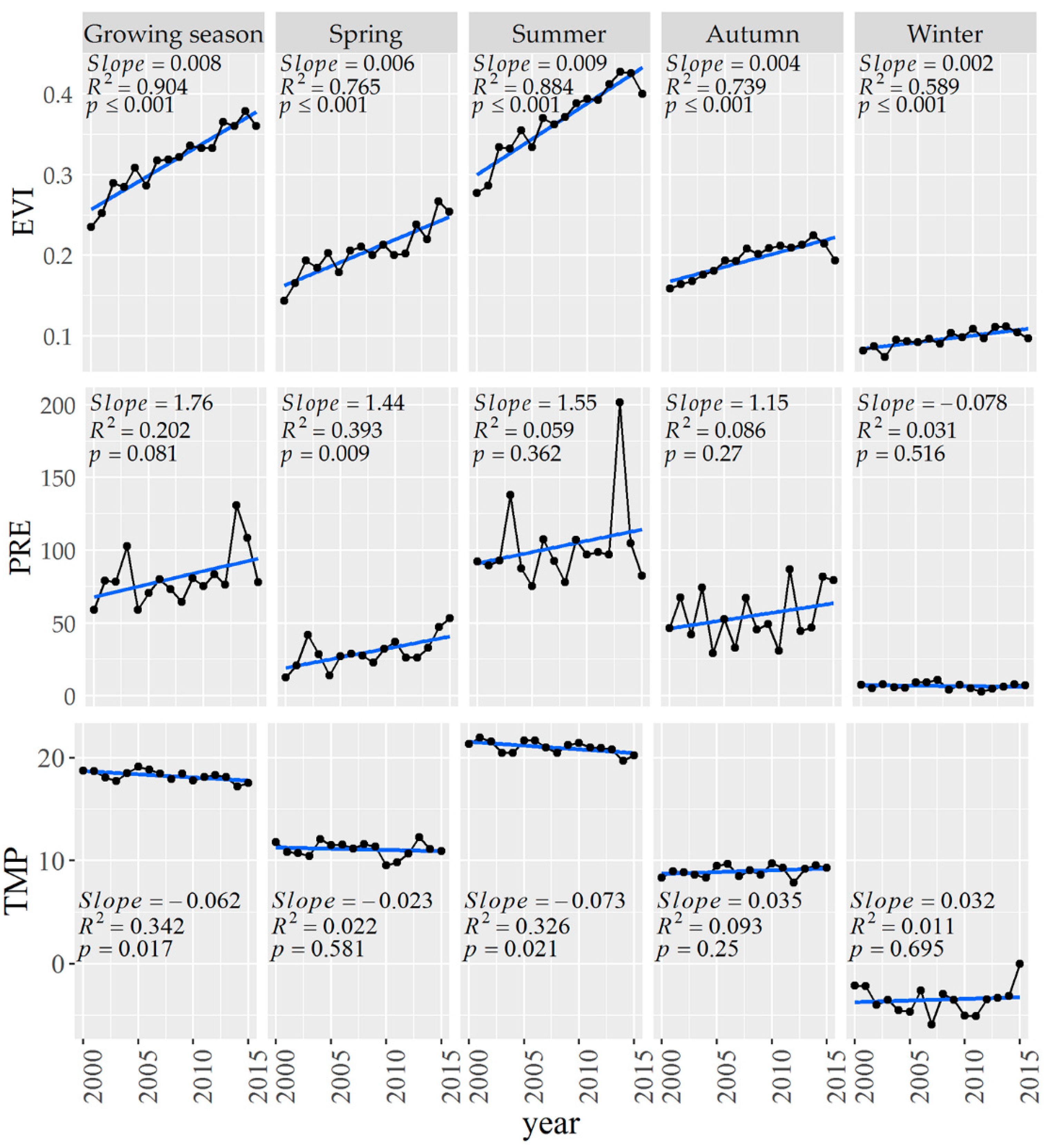
Forests 10 01071 g001
Figure 2. Interannual variation of EVI, mean annual precipitation (PRE, mm), and mean annual temperature (TMP, °C) over 2000–2015 for central Loess Plateau. The seasons include the growing season (April–September), spring (March–May), summer (June–August), autumn (September–November), and winter (December–February). The linear trends were fit by the ordinary least squares method.
Forests 10 01071 g002
Figure 3. Spatial distribution of EVI (/year), precipitation (mm/year) and temperature (°C/year) trends in the study area during the period 2000–2015. (a)–(d) show the EVI trend for the growing season, spring, summer, and autumn, respectively. (e)–(h) and (i)–(m) are respective precipitation and temperature trends for the same four study periods as (a)–(d). Regions with red hatching in (e)–(m) designate the trends are significant trends.
Forests 10 01071 g003
Figure 4. Spatial distribution of EVI dynamics consistency during 2000–2015. (ad) show consistency types of EVI dynamics for the growing season, spring, summer, and autumn, respectively. (eh) are spatial distributions of the Hurst exponent for the growing season, spring, summer, and autumn, respectively.
Forests 10 01071 g004
Figure 5. Variations of the correlation coefficient and partial correlation coefficient between EVI and climatic factors among different months (January–December) with a 16-year moving window in 2000–2015. (a) Correlations between EVI and PRE (precipitation, mm/year). (b) Correlations between EVI and TMP (temperature, °C/year). * and ** represent a p-value < 0.05 and p-value < 0.01, respectively.
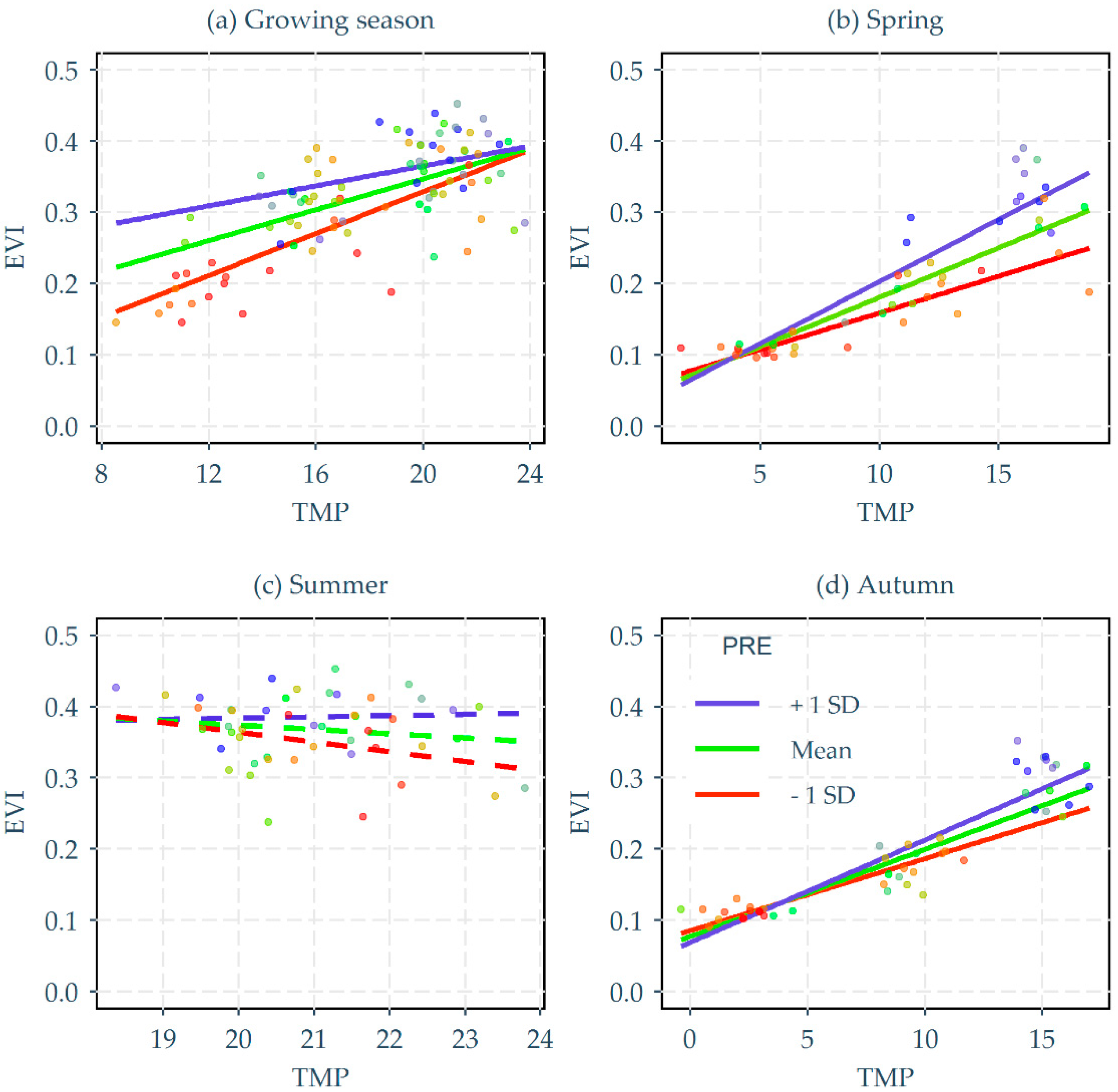
Forests 10 01071 g005
Figure 6. Predicted effects of the interactions between temperature (TMP, °C) and precipitation (PRE, mm) on EVI for the growing season, spring, summer, and autumn, respectively using simple-slope analysis for 2000–2015. Precipitation was treated as a continuous moderator and depicts the mean of precipitation, and the mean minus and plus one standard deviation (SD). The dashed lines represent non-significant simple slopes. The points are the monthly values averaged across the entire study area.
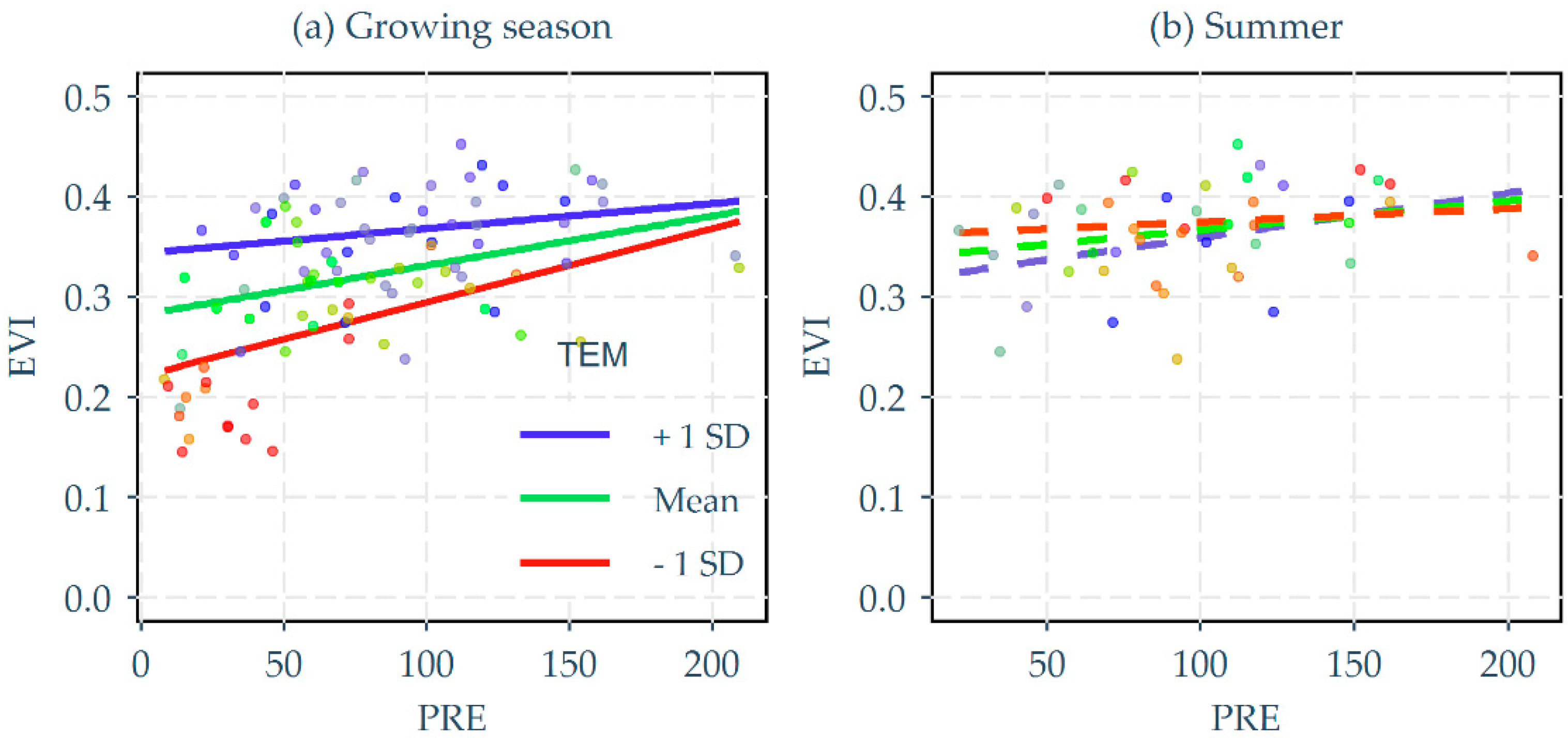
Forests 10 01071 g006
Figure 7. Predicted effects of the interactions between precipitation (PRE, mm) and temperature (TMP, °C) on EVI for the growing season, spring, summer, and autumn respectively using simple-slope analysis for 2000–2015. Temperature was treated as a continuous moderator and depicts the mean of temperature, and the mean minus and plus one standard deviation (SD). The points are the monthly values averaged across the entire study area.
Forests 10 01071 g007
Figure 8. Spatial distribution of correlation coefficients between EVI and climate factors in the study area during 2000–2015. (ad) show the correlation coefficients between EVI and precipitation (PRE, mm) for the growing season, spring, summer, and autumn, respectively. (eh) portray the correlation coefficients between EVI and temperature (TMP, °C) with the same four study periods as (ad).
Forests 10 01071 g008
Figure 9. Predicted effects of the interaction between temperature (TMP, °C) and precipitation (PRE, mm) on EVI for growing season and summer respectively without the extreme precipitation values (>400 mm) using simple-slope analysis for 2000–2015. The temperature was treated as a continuous moderator and depicted the mean of temperature, the mean minus and plus one standard deviation (SD). The points are the monthly values averaged across the entire study area.
Forests 10 01071 g009
Table 1. Classification criteria for consistency in vegetation growth dynamics.
SEVIZHurst ExponentVariation Types
≥0.0005<−1.96>0.5Consistency and significant increase
≥0.0005−1.96 to 1.96>0.5Consistency and slight increase
−0.0005 to 0.0005−1.96 to 1.96>0.5Consistency and stability
<−0.0005−1.96 to 1.96>0.5Consistency and slight degradation
<−0.0005≥1.96>0.5Consistency and severe degradation
<0.5Undetermined future variation trend
Table 2. The significant differences in the distribution of Hurst exponents between land cover classes using a one-way simple ANOVA test for the growing season, spring, summer, and autumn, respectively. Compared land cover classes included forest and crop, forest and grassland, and crop and grassland. *** represents a p-value < 0.001.
SeasonsCompared Land CoversF Valuesp-Values
Growing seasonForest and crop850.2<0.001 ***
Forest and grassland3091<0.001 ***
Crop and grassland475.3<0.001 ***
SpringForest and crop3585<0.001 ***
Forest and grassland5493<0.001 ***
Crop and grassland23.7<0.001 ***
SummerForest and crop160.1<0.001 ***
Forest and grassland247.9<0.001 ***
Crop and grassland907.1<0.001 ***
AutumnForest and crop9941<0.001 ***
Forest and grassland10506<0.001 ***
Crop and grassland139.6<0.001 ***
Table 3. Average Hurst exponent of forest, grassland, and crop for the growing season, spring, summer, and autumn respectively during 2000–2015.
Hurst ExponentGrowing SeasonSpringSummerAutumn
Forest0.65070.61070.63980.6142
Grassland0.65690.62170.64400.6305
Crop0.65450.62100.64170.6324
Table 4. The significant differences in the distribution of EVI at the selected precipitation levels (i.e., mean + SD, mean, mean − SD) using one-way ANOVA analysis for the growing season, spring, summer, and autumn, respectively. Precipitation was considered as the moderator. *** represents a p-value < 0.001.
SeasonsF Valuep-Value
Growing season12<0.001 ***
Spring14.73<0.001 ***
Summer2.520.09
Autumn17.62<0.001 ***
Table 5. The significant differences in the distribution of EVI between the selected precipitation levels (i.e., mean + SD, mean, mean − SD) using one-way simple ANOVA analysis for the growing season, spring, summer, and autumn, respectively. Precipitation was considered as the moderator. Compared precipitation levels include mean + SD and mean, mean + SD and mean − SD, and mean and mean − SD. * and *** represent a p-value < 0.05 and p-value < 0.001, respectively.
SeasonsCompared PRE LevelsF Valuep-Value
Growing seasonMean + SD and mean0.220.64
Mean + SD and mean − SD21.41<0.001 ***
Mean and mean − SD4.130.047 *
SpringMean + SD and mean1.410.25
Mean + SD and mean − SD29.28<0.001 ***
Mean and mean − SD2.270.14
SummerMean + SD and mean00.98
Mean + SD and mean − SD4.760.03 *
Mean and mean − SD0.690.41
AutumnMean + SD and mean0.070.80
Mean + SD and mean − SD35.48<0.001 ***
Mean and mean − SD14.81<0.001 ***
Table 6. The significant differences in the distribution of EVI at the selected precipitation levels (i.e., mean + SD, mean, mean − SD) using one-way ANOVA analysis for the growing season, spring, summer, and autumn, respectively. Temperature was considered as the moderator. The selected temperature levels include mean + SD, mean, and mean − SD. *** represents a p-value < 0.001.
SeasonsF Valuep-Value
Growing season39.32<0.001 ***
Spring26.29<0.001 ***
Summer1.030.37
Autumn46.99<0.001 ***
Table 7. The results of one-way ANOVA test on EVI at three selected temperature values (i.e., mean + SD, mean, mean − SD) in the growing season, spring, summer, and autumn, respectively. Temperature was considered as the moderator. *** represents a p-value < 0.001.
SeasonsCompared PRE LevelsF Valuep-Value
Growing seasonMean + SD and mean1.120.29
Mean + SD and mean − SD60.1<0.001 ***
Mean and mean − SD71.2<0.001 ***
SpringMean + SD and mean10.5<0.001 ***
Mean + SD and mean − SD158<0.001 ***
Mean and mean − SD20.57<0.001 ***
SummerMean + SD and mean0.0020.96
Mean + SD and mean − SD1.440.25
Mean and mean − SD2.110.16
AutumnMean + SD and mean23.15<0.001 ***
Mean + SD and mean − SD400.5<0.001 ***
Mean and mean − SD23.04<0.001 ***

