Article

Evaluating Model Predictions of Fire Induced Tree Mortality Using Wildfire-Affected Forest Inventory Measurements

1
USDA Forest Service Pacific Northwest Research Station, 620 SW Main St. Ste 502, Portland, OR 97205, USA
2
USDA Forest Service Pacific Northwest Research Station, 3200 SW Jefferson Way, Corvallis, OR 97331, USA
*
Author to whom correspondence should be addressed.
Forests 2019, 10(11), 958; https://doi.org/10.3390/f10110958
Submission received: 6 September 2019 / Revised: 17 October 2019 / Accepted: 23 October 2019 / Published: 27 October 2019
(This article belongs to the Section Forest Inventory, Modeling and Remote Sensing)

Abstract

:
Forest land managers rely on predictions of tree mortality generated from fire behavior models to identify stands for post-fire salvage and to design fuel reduction treatments that reduce mortality. A key challenge in improving the accuracy of these predictions is selecting appropriate wind and fuel moisture inputs. Our objective was to evaluate postfire mortality predictions using the Forest Vegetation Simulator Fire and Fuels Extension (FVS-FFE) to determine if using representative fire-weather data would improve prediction accuracy over two default weather scenarios. We used pre- and post-fire measurements from 342 stands on forest inventory plots, representing a wide range of vegetation types affected by wildfire in California, Oregon, and Washington. Our representative weather scenarios were created by using data from local weather stations for the time each stand was believed to have burned. The accuracy of predicted mortality (percent basal area) with different weather scenarios was evaluated for all stands, by forest type group, and by major tree species using mean error, mean absolute error (MAE), and root mean square error (RMSE). One of the representative weather scenarios, Mean Wind, had the lowest mean error (4%) in predicted mortality, but performed poorly in some forest types, which contributed to a relatively high RMSE of 48% across all stands. Driven in large part by over-prediction of modelled flame length on steeper slopes, the greatest over-prediction mortality errors arose in the scenarios with higher winds and lower fuel moisture. Our results also indicated that fuel moisture was a stronger influence on post-fire mortality than wind speed. Our results suggest that using representative weather can improve accuracy of mortality predictions when attempting to model over a wide range of forest types. Focusing simulations exclusively on extreme conditions, especially with regard to wind speed, may lead to over-prediction of tree mortality from fire.

1. Introduction

Accurate predictions of tree mortality in forests affected by fire are important to land managers and policy-makers charged with planning fuel treatments and assessing risk to life and property if wildfire occurs [1,2]. Estimates of the likelihood of trees dying during, or following, a wildfire can influence decisions about when and how to implement mechanical thinning or other fuel reduction treatments. Managers of forests on public land may seek to balance the risk of trees dying from fire effects against the costs and revenues from forest harvest [3] while also supporting the role that fire-killed trees provide as habitat for insects and birds [4]. Recent increases in damage from wildfire and costs of suppression, and forecasts of future increases driven in part by anthropogenic global warming [5] provide fresh motivation to improve the accuracy of tree mortality prediction.
Predicting post-fire tree mortality based on pre-fire stand conditions is difficult because it typically requires an estimate of fire intensity and its impacts from a fire behavior model. Estimation of fire intensity requires calculation of the rate of combustion that is dependent on fuel surface area and the fuel-air mixture, which is related to particle size and fuel density [6]. These are difficult to measure so the modeling of fire behavior tends to rely on highly-generalized fuel models [7]. Estimates of fuel moisture, air temperature, and wind speed are combined with fuel models to estimate flame length. Tree canopy base height and canopy density are used with flame length to estimate degree of crown scorch, likelihood of crown fire, and subsequent tree mortality.
Forest managers in the western United States commonly use the Forest Vegetation Simulator (FVS) and its Fire and Fuels Extension (FFE) to simulate wildfire effects on stand development and response to management actions [8]. FVS is a modeling framework with 20 geographically distinct variants, each developed using empirical growth data from within its geographical application area to simulate the impact of management over a broad range of forest types and stand structures [9]. The ability to link stand development with disturbances and forecast outcomes of silvicultural treatments has led to FVS-FFE’s widespread adoption as a planning tool for fuels and post-fire management [10]. The FVS-FFE model [8] calculates fire intensity (reported as flame length) using equations formulated by [11] and simulates crown fire spread based on the work of Van Wagner [12] and Scott and Reinhardt [7]. Fire intensity and effects calculations in the model are strongly affected by wind speed and fuel moisture that have long been recognized as the strongest environmental drivers of fire intensity [6]. FVS-FFE uses the Ryan–Amman (RA) equation to relate fire intensity, indicated by flame length, to tree mortality. The RA equation uses crown scorch and bark thickness to predict tree mortality [8]. Crown scorch reflects direct heat damage to foliage while bark thickness serves as a proxy for resistance to fire effects (e.g., cambial heating). While most work on validating the RA mortality model has focused on individual trees, there remains a need to examine mortality at the stand level [13]. Most RA validation studies rely on post-fire crown scorch assessments to evaluate mortality prediction accuracy.
Because forecasting mortality from pre-fire stand conditions requires use of fire behavior models, full validation of the RA equation requires testing over a range of conditions that influence fire behavior. Forest managers in the United States commonly use FVS-FFE to weigh the impact of alternative management scenarios on potential fire behavior and effects as part of planning processes, such as the National Environmental Policy Act (NEPA) process. In such cases, they often use FVS-FFE’s default weather scenarios (e.g., [14]) or percentile-selected extreme weather from local weather station archives (e.g., [15,16]). FFE default weather scenarios are intended to represent fire effects under moderate (POTMod) and severe conditions (POTSev), and are hereafter collectively referred to as POTFIRE scenarios. While one or two such weather scenarios may adequately represent a subset of fires, they may not be representative of most fires, leading to errant fire model predictions. In a rare, published example of validating FVS-FFE’s tree mortality predictions with field data, Hummel [17] found major differences between tree mortality predictions based on observed vs. FFE default weather data. Inaccurate or unrepresentative weather data can lead to errant fire model predictions that preclude reliable evaluation of fuel treatment effectiveness, effective hazard mitigation, or valid post-fire recovery plans [18].
The US Department of Agriculture (USDA) Forest Service’s Forest Inventory and Analysis (FIA) Program maintains and samples hundreds of thousands of forest inventory plots on a systematic grid sample [19,20]. The many fires that encounter these plots, with the potential to affect the vegetation growing there, present a unique and valuable opportunity to improve existing mortality models by testing correspondence between model predictions and measured, empirical outcomes. A major strength of analyzing fire effects using FIA plot data is that vegetation types and fire severities are represented in FIA data in proportion to their frequency in the landscape; in other words, a representative, unbiased sample. Analysts at the Pacific Northwest Research Station’s FIA Program initiated a Fire Effects and Recovery Study (FERS) to re-visit fire-affected plots within one year of fire to assess post-fire tree mortality and fire-effects in California, Oregon, Washington and Alaska [21].
Using FIA pre-fire and post-fire measurements, we sought to understand (1) how accuracy of FVS-FFE’s tree mortality predictions might be improved by replacing FVS-FFE’s default weather scenarios with representative weather scenarios developed from local weather data collected when plots were encountered by fire; and (2) how accuracy varies among species and forest types. We anticipated that mortality predictions making use of representative weather scenarios would be more accurate and that variation in accuracy among species and forest types would indicate areas for model improvement.

2. Methods

2.1. Study Area and Fire Selection

We sampled forests within wildfires that occurred in the states of California, Oregon, and Washington on the west coast of the United States (32.6–49.0° N latitude, 114.2–124.2° W longitude). Forests in this region are found from sea level to over 3000 m elevation with annual precipitation ranging from 25 to over 600 cm. Dominant vegetation ranges from xeric–oak (Quercus sp.) and juniper (Juniperus sp.) forest types to mesic–Douglas-fir (Pseudotsuga menziesii (Mirb.) Franco)) and California mixed conifer, and subalpine–true fir (Abies sp.). In years when funding was available to collect post-fire FERS data on FIA plots, essentially all forested inventory plots on national forests within the boundaries of fires larger than 400 hectares were selected for measurement. Because the FERS was initiated in California, with support from National Forest System Pacific Southwest Region 5 cooperators, and only later expanded to other west coast states, most of the 74 fires sampled, which burned between 2002 and 2015, were in California.

2.2. Vegetation Measurements

FIA plots in the Pacific Northwest are installed with a sampling intensity of one plot per 24 km2, and are distributed among ten spatially balanced panels. One panel of plots is visited and measured each year, and an entire cycle of inventory sampling completed in ten years [19]. In California, the National Forests in the Pacific Southwest Region collect FIA protocol inventory data on additional plots installed in selected forest types [22], and, when these burned, they became candidates for inclusion in the FERS sample. The nationally-standard FIA plot design consists of four 7.31 m radius subplots, where height, diameter, compacted crown ratio, species, and other attributes are assessed on all trees ≥12.7 cm in diameter at breast height (dbh). Trees smaller than 12.7 cm dbh are sampled on a 2.07 m radius microplot within the subplot. Large trees (>75 cm dbh in western Oregon and Washington, >61 cm in California and eastern Oregon and Washington) are sampled on an 18.0 m radius macroplot. Factors computed as the inverse of a plot’s sample areas are used to expand tree measurements on an area basis (e.g., trees and basal area per hectare). With the exception of the California Mixed-Conifer forest type, which is assigned based on the presence of particular species combinations and location, forest type is designated as the species with a plurality of stocking.
On plots occurring within fire boundaries, FIA field crews collected fire-effects data within 1-year post-fire. Pre-fire FIA plot measurements were collected, on average, 4.0 years (0.1 sd) before the fire (range 1 to 10 yrs.). FERS metrics include assessments of mortality, including whether fire-caused, as well as fire effects on ground surface cover, tree boles, and crowns.
We relied on field-assessed bole char height to evaluate the accuracy of FFE-FVS’s estimates of flame length—the metric that serves as a proxy for fire intensity in that model’s mortality predictions [23,24,25]. For every tree larger than 2.54 cm diameter breast height, we calculated tree-level bole char height as the midpoint between the greatest height at which bole char was observed (high char height) and the lowest height at which the bole was observed to have remained free of scorch (low char height), as measured as a length along the bole of the tree from the root collar. A stand-level mean bole char height was calculated as the mean of all tree-level bole char heights on trees for which this attribute was neither zero nor equal to actual tree height; unqualified trees provide no values as “yardsticks” capable of “recording” flame length. All qualifying trees contributed equally in computing this mean, as the intent was to represent stand-level surface flame length, which we would not expect to be significantly affected by tree size or the plot size on which trees of a given size were sampled. The modelled surface flame length output of FVS is intended to represent the average flame length for a stand [26]. We assessed the extent to which modeled flame length tracked observed mean bole char height by computing the error (as modelled flame length—mean bole char height) and, for both all stands and subgroups, mean error and root mean square error (RMSE).
FIA protocols partition a plot into separate “conditions” when a plot contains both forest and non-forest area, straddles a reserved area boundary or contains >1 owner group, forest type, stand size class, regeneration status, and/or tree density class [19]. We relied on condition as the areal analysis unit because we sought to identify and understand patterns of mortality by forest type. Conditions can be thought of as stands, and they were modeled as such in FVS (see below); those occupying less than 20 percent of a plot’s area were excluded as too small (these typically had a tree tally that was too small to adequately represent a forest stand and risked introducing artifacts when calculating tree mortality).
Post-fire measurements were ultimately collected from a total of 443 forested conditions with pre-fire data. Data from Remote Automated Weather Stations (RAWS) required data-cleaning before use as some weather fields were not present for every hour during the representative time period. Data for some RAWS stations also contained apparent error values for weather variables (−90 °F for Temperature for example). Fire progression maps also had errors, such as perimeters showing burned area decreasing, which had to be resolved. Based on trends in progression from previous perimeters, we removed any perimeter timepoint that showed the perimeter shrinking instead of growing or remaining static. We did not impute any missing perimeters (see Section 2.3 for sources of fire perimeter data).
Given the difficulty of matching plots with both fire perimeters and suitable RAWS station data, some stands lacked suitable weather data. After removing stands affected by these issues, there remained 342 stands available for this analysis. Measurements include both standard FIA attributes like diameter and height (Table 1) and others, like bole char height, that were specific to FERS. Each pre-fire condition had been assigned an FIA forest type [27] via data compilation or in the field, but when there were fewer than five conditions in a forest type, we combined types (Supplemental Table S1) to create the 10 forest type groups constructed for this study (listed in Table 1).

2.3. Fire Weather

To obtain weather attributes that potentially represent when each condition burned, we linked data collected by the RAWS network to each forested condition after geoprocessing locations of conditions, RAWS, and approximate daily fire progression perimeters delineated during the fire events to identify the most suitable station for representing the fire behavior and the approximate date and time that a plot burned. Stations in the RAWS network are located in large, open areas, free from obstructions, sources of dust and surface moisture [28] and collect hourly average, minimum, and maximum wind speed, temperature, and humidity, which can be used to predict fire danger metrics via the National Fire Danger Rating System. While not necessarily permanent, most stations do offer many years of weather observations and tend to have the most complete records during fire season. For each plot, we downloaded (http://www.raws.dri.edu/) all RAWS data in the vicinity for the year the fire encountered the plot and used it to calculate hourly fuel moisture (for 1-, 10- and 100-hr fuels) via FireFamilyPlus [29]. We assigned, as the best station for a plot, the one that was closest in both Euclidean space and elevation, with some leeway to also consider intervening geographic features such as mountain ranges that occasionally made a station that was not the closest, as the best choice.
To select the best hourly weather observations, we conducted GIS overlay of shapefiles containing date- and time-stamped fire perimeters from online fire perimeters archives on the plot locations to estimate the timeframe during which the fire likely encountered the plot. Fire perimeters were obtained from the USGS [30]. The fire ignition and containment dates, obtained from InciWeb [31] and CALFire [32], were also helpful in bracketing and selecting the relevant fire progression perimeters, which were separated in time by from a few hours to a few days, though most commonly about a day apart.
Differences in temporal resolution pose a considerable obstacle to linking fire progression maps and RAWS observations. The mean, over all plots, progression perimeter interval of 37 h is considerably greater than the 1-h RAWS interval. In an attempt to reduce this scale disparity, we assigned each plot to a spatial quartile via visual assessment of the progression perimeters that bracket a plot, assuming a constant fire growth rate during the progression interval. In thirty-three plots with intervals under four hours, there was no need to assign a quartile and all 2–4 h of weather observations were used. To account for variation within the assigned quartile (or less than 4-h interval), we calculated the mean, minimum, and maximum values for the observed, hourly weather attributes within the assigned quartile. These means, minimums and maximums for wind speed, temperature, and fuel moisture were arranged in three representative weather scenarios designed to reflect the range of weather conditions, for use as input to the FFE model (Table 2).

2.4. FVS Modeling

The Forest Vegetation Simulator (FVS) is an empirically-based, distance-independent, individual tree growth and yield model, which treats the stand as the population unit [9] (Dixon 2013). The Fire and Fuels Extension (FFE-FVS) to FVS can simulate fire effects accounting for weather, slope and fuel structure information supplied via tree list and stand characteristic data and user provided parameters. Of interest for this study are FFE-FVS’s predictions of tree mortality, which are often relied upon by managers interested in how fire hazards might be reduced or stand resistance increased in response to silivicultural activities such as fuel treatments. To evaluate prediction accuracy, we loaded pre-fire FIA data for all 342 conditions into FVS as stands.
FFE estimates post-fire tree mortality via two submodels [8]. The fuel submodel tracks surface and crown fuels (as parameterized by canopy bulk density and canopy base height), using logic intended to assign two [33] (Anderson 1982) “default” fire behavior fuel models and associated weights, typically based primarily on forest type, though specifics vary among FVS variants. For this study, we relied on the default fuel models assigned by FFE. The fire intensity and fire effects submodel estimates flame length and fire type (e.g., surface, active crown) based on the fuel model, weather parameters, slope, and crown fuels. For the weather scenarios, flame length was taken from the Burn report output table while the flame length for the POTFIRE scenarios was taken from the POTFIRE output table. As the Burn report table only reports total flame length (surface and crown fire combined), we selected total flame length from the POTFIRE table. FFE’s predictions of mortality are based on the Ryan–Amman (RA) equation which models tree mortality as a function of crown scorch and bark thickness [34]. FFE first calculates mortality probability from surface fire and then adds additional mortality from predicted crown fire activity. Mortality is expressed in terms of the percent of pre-fire live-tree basal area (m2/ha) that died due to fire effects. FVS-FFE takes the probability of mortality and reduces the basal area (BA) of the individual tree, which is then aggregated to produce a stand-level summary of BA killed by fire. For example, a tree with a 0.5 mortality probability would have its BA reduced by 50%. Trees with 100% crown scorch, from a simulated crown fire for example, are considered dead, resulting in 100% BA loss [8]. FFE users can test the influence of variations in fire intensity on tree mortality by adjusting keywords that alter fire behavior, for example, air temperature, wind-speed, and the amount and moisture content of fuels’ inputs.
To evaluate the accuracy of predicted mortality in response to the weather scenarios, without regard to forest type group, we compared mortality observed at the post-fire FIA visit with FVS’s estimate of stand-level tree species mortality provided in the FVS Mortality output table. The potential fire report does not list mortality by tree species and so species specific mortality could not be compared to observed mortality for the POTFIRE scenarios.
We used the FVS-FFE SIMFIRE keyword to model wildfires using the three RAWS derived weather scenarios as well as running SIMFIRE with FFE’s default scenarios’ parameters. The Min Wind scenario is effectively a zero-wind scenario given that the minimum hourly wind measurement for 99% of the weather intervals was zero. Mean weather parameters for the three RAWS derived scenarios and the two POTFIRE scenarios cover a broad range of weather under which fires occur (Table 3).

2.5. Model Assessment

We used mean error (i.e., bias), root mean squared error (RMSE), and mean absolute error (MAE) of stand-level percent basal area mortality to evaluate prediction accuracy under each of the five weather scenarios (three RAWS based representative weather scenarios and two FFE default scenarios) relative to observed mortality. FVS-FFE estimated mortality estimates at stand and tree levels were obtained from the FVS Mortality table for the SIMFIRE simulations (conducted for the representative weather) and from the POTFIRE table for simulations conducted with FFE default POTFIRE scenarios. We assessed basal area mortality as the percentage of pre-fire BA (m2/ha) killed by wildfire: (BA killed/prefire BA) × 100. Error in % BA killed is defined as the difference between predicted and observed % BA mortality. We applied FFE estimates of stand-level crown scorch height to measured tree heights and crown ratios to calculate predicted tree crown scorch (% of compacted crown length estimated as scorched and burned) for comparison to field-assessed crown scorch. To evaluate accuracy of FFE’s flame length estimates, error was defined as predicted flame length minus mean bole char height. For bole char and crown scorch, stand-level metrics were obtained by averaging the tree-level observations to the stand-level.
Results were grouped for analysis separately by forest type group and by tree species (for species with at least 500 live trees in the pre-fire dataset) (Table 4). The level of error in forecasting mortality that might be considered acceptable depends on objectives; however, accuracy of at least 70% is an accepted minimum standard for operational and forest planning models [35]. Given the broad geographical scope of the fire-affected fire plots, we selected 30% RMSE as our acceptance standard for stand-level mortality. The mortality errors for the Max Wind and POTSev scenarios were not normally distributed, with a skew towards large overpredictions of mortality. Under non-normal distribution of errors, RMSE is a conservative estimate of error as this metric is quite sensitive to and can be biased by outliers [36]. For the purposes of the study, we accepted this bias as it would penalize scenarios with extreme errors in mortality predictions. We also included MAE as a relevant metric that is less sensitive to outliers.
We used regression trees to assess, independently of FVS-FFE, the relationship of the RAWS weather and stand structure inputs with observed stand-level mortality. The response variable was observed mortality and the predictor variables were stand characteristics (Table 1) and weather parameters from the three representative weather scenarios (Table 3). The R package rpart 4.1 was initially run using default settings, with a minimum number of observations to split a node at 20. Node splits must decrease overall lack of fit of the model by a specified complexity parameter, initially set at 0.01 [37]. To further prevent overfitting, the initial tree is pruned using an optimal complexity parameter selected from the number of node splits with lowest cross-validated error.

3. Results

3.1. Mortality Patterns

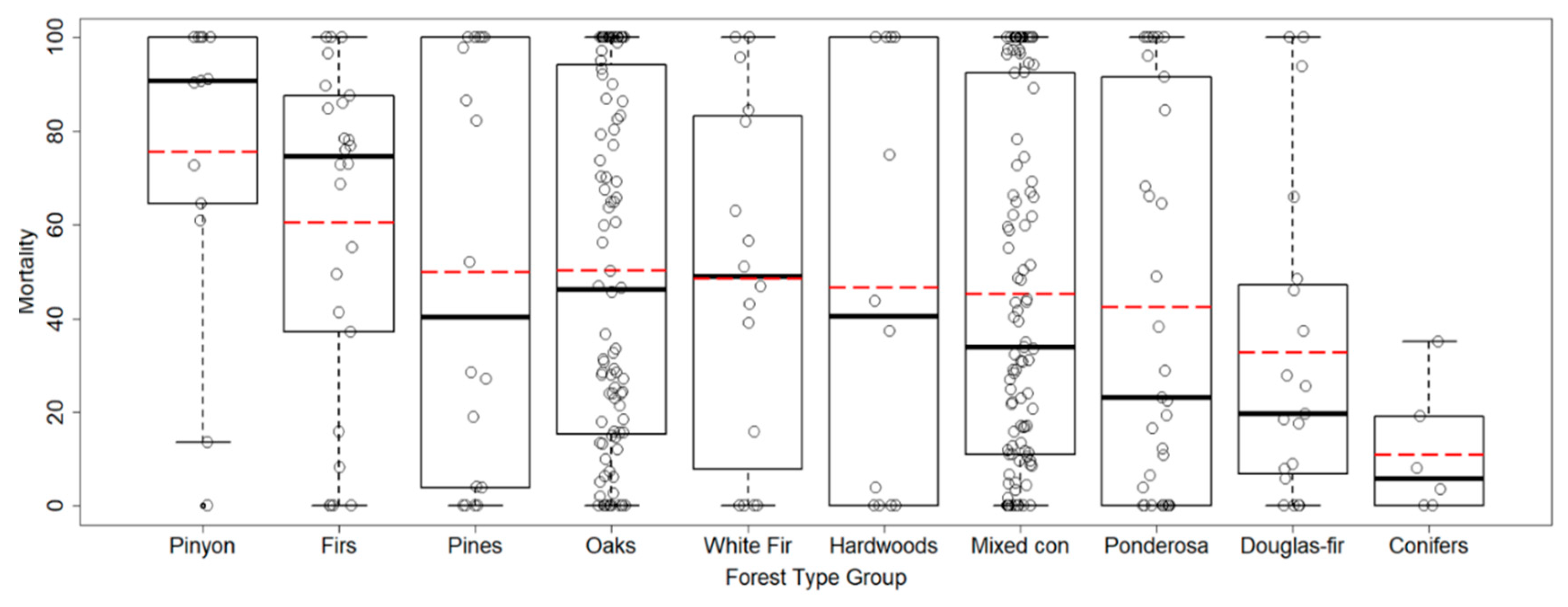
Stand mortality for all stands, expressed as a percent of live basal area that would die, was 48% (39% sd). For seven forest type groups, observed mean BA mortality fell between 40% and 60% (Figure 1). The inter-quartile ranges spanned 80% for many types, including the three forest type groups with the most stands (California Oaks, Mixed Conifer, and Ponderosa Pine). Mortality was <10% for twenty-four percent of the stands, and ≥90% for another 27%. Mortality rates tended to be lowest in the Other Conifers and Douglas-fir groups (median of 6 and 20%, respectively), and highest in the Pinyon-Juniper and Fir groups (median of 91 and 75%, respectively). Means exceeded medians in most forest type groups, owing to the high frequency of stands with 100% mortality.

3.2. Accuracy of Mortality Predictions by Weather Scenario

Across all stands, the Mean Wind scenario was the most accurately predicted stand level mortality rate, with the lowest mean error (+4%), and with RMSE and MAE comparable to the POTMod and Min Wind scenarios (Table 5). The POTSev and Max Wind scenarios over-predicted mean mortality by over 20%, while the POTMod and Min Wind scenarios under-predicted mortality by at least 10%. The high RMSEs of all the weather scenarios indicate poor predictive ability at the stand scale; Pearson correlation coefficients (r) between predicted and observed percent basal area mortality ranged from 0.15 for Mean Wind to 0.28 for POTMod. The scenarios with the lowest predicted mean mortality (POTMod and Min Wind) also had the lowest RMSE and MAE values. All scenarios except for Max Wind had MAE within 5% of POTMod, and the RMSE for Min Wind was within 5% of POTMod as well.
The most accurate weather scenario differed among forest type groups, with Mean Wind having the lowest error for five groups, POTMod for four groups, and Max Wind for one (Table 6). The Mean Wind scenario had the lowest error for the most abundant conifer types (California mixed conifer and Ponderosa pine), while the POTMod scenario had the lowest errors for the hardwood types (California oaks and other hardwoods). The high mortality rates of subalpine forests in the Firs group were most accurately modeled with the Max Wind scenario.
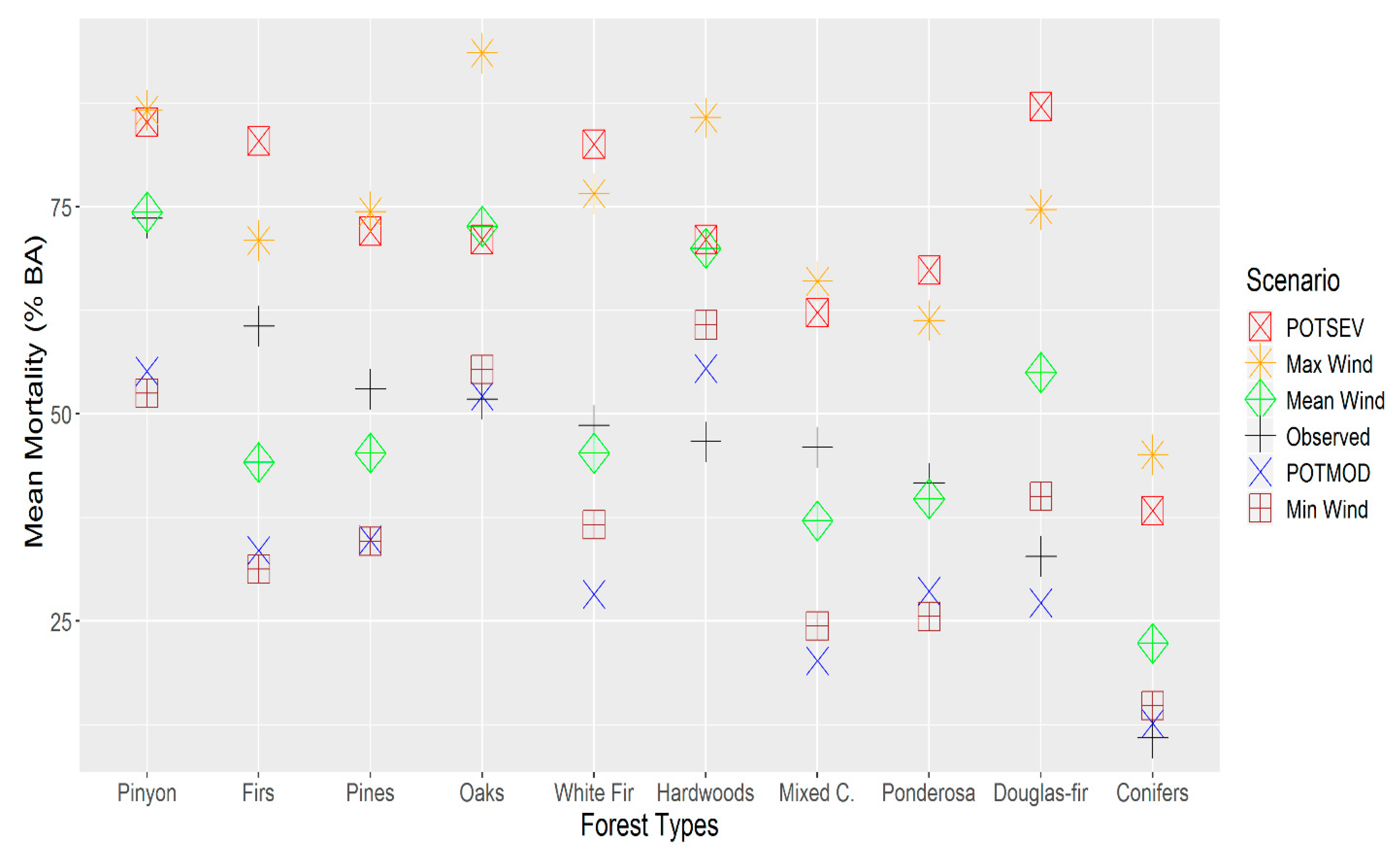
For most forest type groups, the POTMod or Min Wind scenarios had the lowest RMSE (Table 6). These scenarios also had the lowest estimated mortality levels, with means exceeding 35% BA mortality only for California oaks, other hardwoods, and Pinyon/juniper forest type groups (Figure 2). However, for most of the forest type groups, the weather scenario with the lowest mean error also had an RMSE within 3% of the lowest RMSE (e.g., California mixed conifer, Table 6). Because RMSE penalizes large errors more than the other metrics, we examined the percentage of stands with over 50% absolute error by forest type group and weather scenario. The percentage of stands with errors greater than 50% was greatest in the Max Wind and POTSev scenarios for several of the largest forest type groups: California mixed conifer, California oaks, and Douglas-fir (Figure S1). However, even in the Mean Wind scenario, six of the forest types had over 30% of the stands with 50% or greater prediction error.
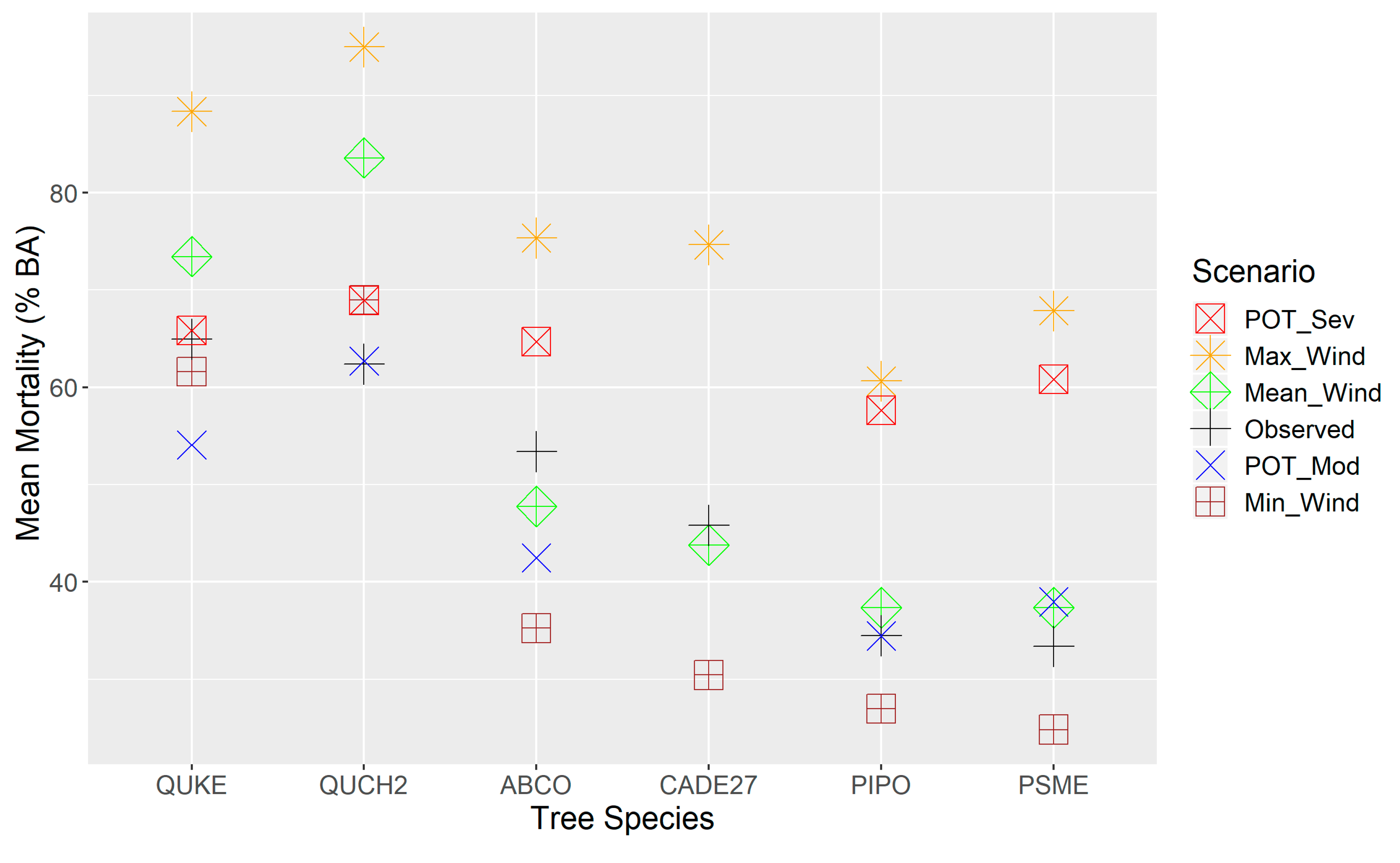
The most accurate weather scenarios for predicting mortality also varied at the tree species level. The Mean Wind scenario produced the lowest mean error for white fir (Abies concolor (Gord. & Glend.) Lindl. Ex Hildebr.), incense-cedar (Calocedrus decurrens (Torr.) Florin), Ponderosa pine (Pinus ponderosa P.&C. Lawson), and Douglas-fir, while the Min Wind scenario had the lowest mean error for canyon live oak (Quercus chrysolepis Liebm.) and California black oak(Quercus kelloggii Newberry) (Figure 3). Mean observed stand-level mortality was close to 60% for both hardwood species, near 50% for white fir and incense-cedar, and less than 35% for Douglas-fir and Ponderosa pine. The Min Wind scenario performed best in reducing RSME and MAE (Table 7).

3.3. Consistency of Model Predictions with Field-Measured Crown Scorch and Bole Char

The distribution of observed stand-level crown scorch resembled that for observed mortality, with a skew towards 100% in the highest mortality forest type groups (Figure S2). As with mortality, mean error for crown scorch was lowest for the Mean Wind scenario, but variability among stands was so great that all five scenarios had RMSE and MAE values within 5% of Mean Wind (Table 8), with a range of crown scorch RMSE (47–51%) comparable to that for mortality RMSE (42–54%), and errors in predictions of these variables were closely related. The most accurate weather scenario for estimating crown scorch varied among forest type groups. The Max Wind and POTSev scenarios had the lowest RMSEs in the high-mortality pinyon/juniper, firs, and pines forest type groups, while the Mean Wind or POTMod scenarios had the lowest RMSEs for the abundant California mixed conifer, Ponderosa pine, and white fir forest type groups (Figure S3).
The mean stand-level bole char height across all stands was 3.3 m (3.0 sd), although it was not unusual for stands in several forest type groups to have bole char heights exceeding 5 m (Figure S4). When predicted flame length under the five weather scenarios was evaluated against these bole char observations, patterns of error resembled those for mortality, with moderate scenarios predicting flame length lower than the measured bole char heights and severe weather scenarios predicting the opposite (Table S2). The Min Wind and Mean Wind had the lowest mean errors across most forest type groups while Mean Wind and POTMod had the lowest RMSE across most groups.

3.4. Importance of Factors That Contribute to Stand-Level Tree Mortality

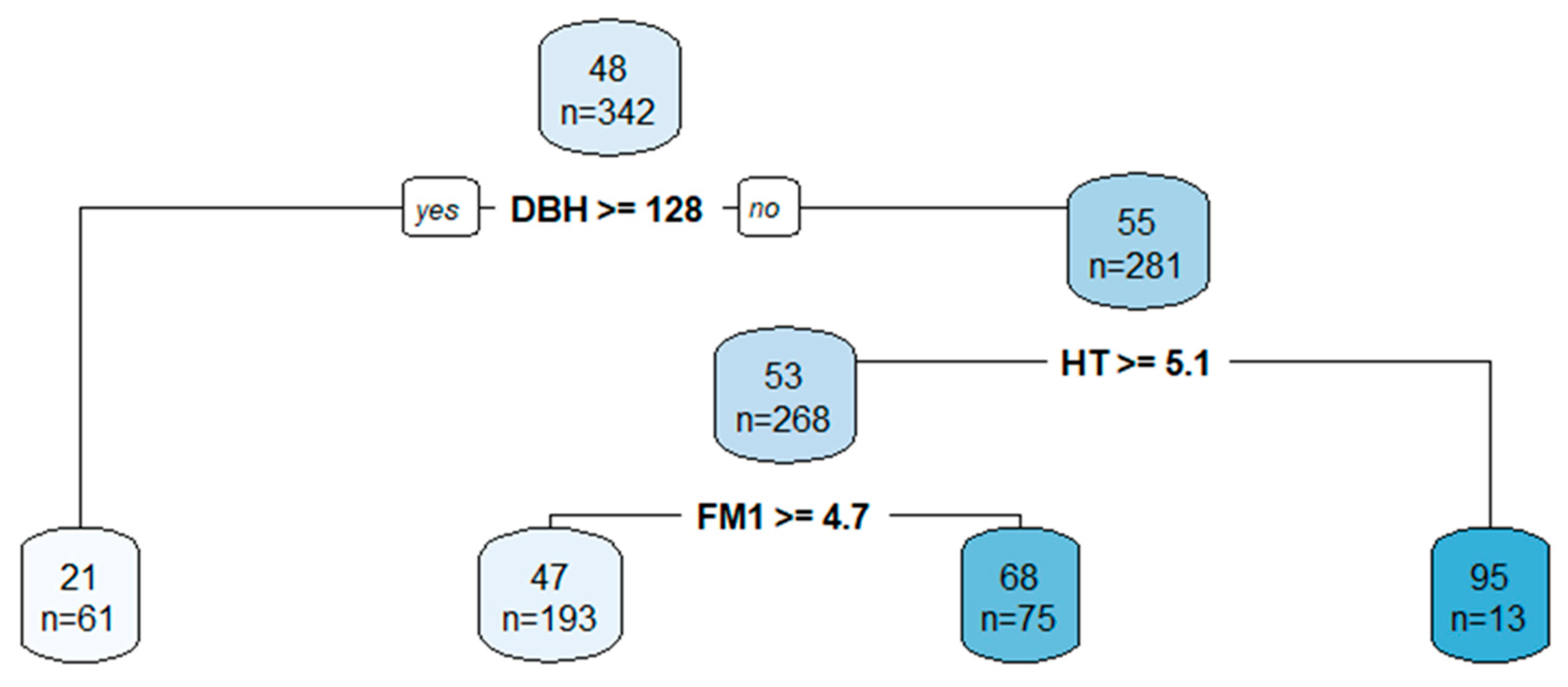
The regression tree modeling revealed strong relationships between stand and weather attributes and stand-level mortality. The model with the lowest error had three splits with a complexity parameter of 0.03, and identified mean 1-hr fuel moisture, mean DBH, and mean stand height as major drivers of mortality (Figure 4). The first spilt was driven by stands with a mean DBH ≥128 cm having low mortality (21%). For the remaining stands, stands with mean stand height of less than 5.1 m had much high mortality (95%) than those with a higher mean stand height (53%). The next spilt was driven by mean 1-hr fuel moisture. Stands with ≥5% 1-hr fuel moisture had 47% mortality compared to 68% when below 5%.
A separate regression tree analysis using the error in stand level mortality for the Mean Wind scenario as the response variable indicated that FFE substantially over-predicted mortality on steep slopes, with a mean error of 38% on slopes >68% (Figure S5). FFE also over-estimated mortality for small-diameter stands (mean dbh < 8.5 cm), but was quite good for larger-diameter stands on moderate slopes (43–68%). The model under-predicted mortality on gentle slopes (slope < 43%).

4. Discussion

4.1. Assessment of Representative Weather Inputs vs. FFE’s Defaults

Our expectation that representative weather scenarios would produce more accurate predictions was partially confirmed. The Mean Wind representative weather scenario resulted in the lowest mean error overall, and for most forest type groups and tree species. However, contrary to expectations, the default FVS-FFE moderate burn scenario (POTMod) had the lowest RMSEs, primarily by providing a better match than representative weather scenarios where observed mortality was low.
Accuracy of mortality prediction at stand scale was quite variable. Judged by mean absolute error (MAE), all five weather scenarios had success within five percentage points of our 30% error maximum target in at least two forest types while for nine of the forest type groups, MAE was below 33%. By contrast, RMSE of differences between predicted and observed exceeded 40% for all five weather scenarios. A key distinction between MAE and RMSE is that the latter more severely penalizes errors with the greatest magnitude [36]. In all five scenarios, there were many stands for which discrepancy between predicted and observed mortality was very large, and this is apparent in the many cases with RMSE > 50%. Even with the best scenario, Mean Wind, predictions for 30% of stands were off by more than 50% in six of the forest type groups.
We expected that weather parameters more representative than those in FFE’s default scenarios would reduce prediction errors in fire behavior [38,39]. Errors in predicting fire behavior like flame length lead to errors predicting fire effects like crown scorch, and lead, in turn, to errors in predicting mortality. Flame length predictions from the three more temperate weather scenarios appear to be more accurate and credible, based on comparison with median bole char heights. However, relying on such an indirect indicator of fire intensity warrants caveats. While flame height suggested by bole char height may approximate flame length under low wind speed on gentle terrain [40], departure from these conditions, for example, with respect to slope, fuel bed depth, and wind speed, can degrade this approximation. For example, bole char extends higher on steep slopes, irrespective of flame length [41]. Nonetheless, much of the error in over-prediction in tree mortality in the MAXWind and POTSev scenarios stemmed from an over-estimation of fire intensity resulting from a combination of high winds and steep slopes. Our regression tree analysis highlighted greater over-prediction errors on very steep slopes (>68). The Rothermel surface fire model was originally intended to model surface fire spread on flat terrain, with later attempts to modify the model by increasing fire intensity on steeper slopes [8,42]. Our results suggest that the model as implemented in FVS-FFE has difficulty representing fires on steep slopes and under high winds.
Despite wind being represented in FFE as the strongest driver of fire behavior [8], fuel moisture inputs appeared to play a greater role in our results than wind. Given the greater predictive power of the Mean Wind scenario, with POTMod and Min Wind not far behind, it appears that most of the benefits of using representative weather, rather than FFE defaults, can be attributed to the dead fuel moisture parameters and their influence on flame length prediction, rather than wind speed. At low wind speeds between 0 and 4.5 m/s, FFE, predicts little difference in fire intensity [43]. The regression tree results provide additional support for the greater role of fuel moisture, since at very low moisture (<5% for 10-hr fuels), mortality was much greater (68%) than at higher fuel moisture. In FVS-FFE, low fuel moisture facilitates transition from surface to crown fire, even with low wind speeds, thus elevating the likelihood of mortality [7,8]. At the same time, in flatter stands (<43% slope), the regression tree provided evidence that high estimated fuel moisture resulted in under-estimation of mortality seen in the Min Wind scenario. Other limitations inherent in FVS-FFE’s fire behavior models may have also contributed to the underprediction by the Min Wind and POT Mod scenarios. Cruz and Alexander [44] reported that rate-of-spread (ROS) predictions for surface fire (using the Rothermel model) and crown fire (using the Van Wagner model) were frequently underestimated. Moreover, the coupled Rothermel–Van Wagner models tend to under-predict transition of surface fire to crown fire in conifer forests [45]. These known model biases have the potential to under-predict mortality by under-predicting fire intensity, and thus the crown scorch input to the mortality model. Surface fire ROS is important because flame length increases with ROS at low wind speeds before plateauing at higher wind speeds when fuel moisture is high [46]. At the same time, underestimation of the transition of surface to crown fires might also be contributing to under-prediction in the Min Wind and POT Mod scenarios. Whether a fire is heading or backing up or down slope can also affect intensity and flame lengths [47]; however, FVS-FFE only models head fires [8].
Our discussion so far assumed that our “representative weather” wind estimates are accurate depictions of the fire environment when FIA plots were affected. Given that the nearest station is sometimes tens of miles away from the FIA plots, RAWS observations, especially wind speeds, are imperfect proxies for the weather on the plots when fire arrives. While it is at least theoretically possible to generate interpolated or meso-scale adjusted wind speed estimates using advanced models, topographic complexity—mountain ranges, elevation differences, wind-protected areas—pose challenges to accuracy. Page et al. [48] tested the accuracy of the National Digital Forecast Database used by fire modelers with RAWS station measurements and found that the model tended to underestimate wind speeds when winds speed exceeded 4 ms−1. More accurate downscaling might provide better weather inputs for future validation efforts. However, the temporal uncertainty on when, exactly, fire encountered the plot makes it difficult to pin down the best hour or hours of RAWS observations to use. Moreover, there may be limits to how well the models underlying FVS-FFE can use improved wind inputs as wind effects on wildfire rate of spread and flame lengths are modeled quite simply compared to other models (FARSITE e.g., [49]) or latest fire physics models [50].
Beyond weather inputs, fuel models are used to represent pre-fire conditions that influence fire behavior [46]. In this study, we allowed FVS-FFE to select the fuel models, which vary by forest type. We did experiment with selecting fuel models based on fuel load data from the inventory plot, but the fuel models selected and results were typically not much different, which is consistent with other studies which report limited benefits to simulated fire behavior accuracy from customizing fuel models based on field-measured fuel loading [51].
We found that the most predictive weather scenario varied by forest type group. The more severe weather scenarios produced the lowest prediction RMSEs in the Juniper/Pinyon and Pines forest type groups, though RMSEs exceeded 40%. Mortality has been observed to be highly variable in Pinyon-Juniper owing to high variability in fuel loads and vegetation composition [52], and these species’ thin bark make them comparatively vulnerable to lethal cambial heating, though survival remains possible where surface fuels and/or tree cover are sparse [53]. The Firs and Ponderosa pine forest type groups had the lowest prediction RMSE with the Min Wind scenario, possibly reflecting higher fuel moisture in these forest types than predicted.
The evaluation of FVS-FFE’s mortality predictions is complicated by challenges imposed by the spatial scale of the FIA plot. The bi-modal distribution of observed mortality (high frequencies of 0 and 100%) could reflect fire effects in within-stand patches rather than the mean effect across individual stands. Conditions adjacent to FIA plots may also introduce variation in fire effects, for example local topographic features that amplify (e.g., a canyon headwall acting as a chimney) or mitigate (e.g., a wind-protected spot) fire behavior. A strength of FIA data is that it reflects the full variation in forest conditions visited by fire, in proportion to how to their occurrence in the landscape. However, parameterization of the FFE was not based on a probability sample from the Pacific Northwest and California, so some FIA conditions may occur in what are essentially “gaps” in the continuum of forest conditions represented in the data from which the FFE model parameters were derived.

4.2. The Role of RA Equation and Tree Species Effects

As the only species-specific parameter in the Ryan and Amman [54] mortality model (RA), the bark thickness coefficient (which is multiplied by tree diameter to estimate bark thickness) is intended to account for species-specific resistance to fire-induced cambial injury [55] and can be interpreted as inversely correlated with probability of cambium death [35,54]. In an assessment of the RA equation on first-order mortality after prescribed fire on National Park lands in the western U.S., Kane et al. [56] found that the RA equation over-predicted mortality for species with thin bark, under-predicted for trees with thick bark, and wasn’t very accurate for any tree with bark <1 cm thick. The most abundant species in this study included trees relatively resistant to fire (Douglas-fir, incense cedar, Ponderosa pine), moderately resistant (white fir, tanoak), and not resistant (California black oak, canyon live oak). Mortality prediction RMSE declined as bark thickness coefficient decreased such that canyon live oak had the lowest RMSE. Bark thickness appears to be a good predictor of first-order mortality, but the assumed linear relationship between bark thickness and tree diameter is not always correct [55]. Zeibig-Kichas [57] found FVS-FFE tended to under-predict bark thickness in California conifers, which would lead to over-prediction of mortality [1,56], but empirical evidence for this effect is lacking given limited data on bark thickness.
In this study, thin-barked canyon live oak was the only species for which mortality was over-predicted by all three representative weather scenarios. While errors in estimation of bark thickness or its effect on mortality may be partly responsible, hardwoods like this have the additional complication in top-killed trees with 100% crown scorch. Even if aboveground plant tissues are dead, new stems and leaves from underground plant tissue will commonly emerge [58], but this does not convert the tree’s status to live under the FIA protocol. However, any tree that sprouts living tissue above the point of diameter measurement is considered a survivor under FIA measurement protocol (as opposed to basal sprouts, which count as new trees). Considering surviving trees included in this study that experienced any crown scorch, we found that 2.8% of the canyon live oak trees had 100% crown scorch, but most had recovered with live crown ratios over 10%. Fewer than 1% of the surviving burned trees of the other species discussed here had recovered from 100% crown scorch. Canyon live oak is increasing in basal area despite increased fire activity in California, possibly due to exploiting niches in unburned stands where fuels are sparse and to its shade-tolerance [59].
Average observed mortality for the more fire-resistant California black oak was no less than for the thinner barked canyon live oak; other studies report comparable mortality rates of about 60% [13,60]. The best RMSE scenario slightly under-predicted mortality, suggesting that resprouting of heavily-scorched trees was not as strong a factor as in canyon live oak. Nevertheless, basal sprouting can greatly affect post-fire stand dynamics, with up to 70% of the top-killed black oak resprouting in one study [13]. California black oak has been experiencing a decline in basal area in California [59], in part due to conifer encroachment into black oak canopies resulting in greater crown-fire caused mortality [61].
FFE’s mortality predictions have several limitations, some of which can be overcome. First, crown scorch is less effective than fire residence time in predicting mortality for species that re-sprout and for small trees [55]. Second, the RA equation does not account for heat-induced root damage, which is a significant mortality mechanism in ecosystems like Ponderosa pine [55,62]. Third, the development and validation of the RA equation focused on conifers and largely excluded hardwoods [1,55], so expanding coverage of fire effects on species beyond major conifer species, such as Douglas-fir and Ponderosa pine, would be a major contribution to accuracy improvement and could build on the work now underway to improve mortality models for southern hardwoods [63,64]. Although the ability of the model to predict mortality for the major hardwood and softwood species was similar in this study, the route to improving model performance will likely require different variables for different species (e.g., root damage for Ponderosa pine as noted above).

4.3. Model Evaluation and Improvement in the Context of Forest Management

There are alternative ways to interpret model errors depending on objectives. Because it is based on a squared error term, RMSE gives greater weight to large errors than to small ones. The direction of error (under vs. over prediction) is also important. In some management contexts, over-prediction of tree mortality, as we observed occurring with the Max Wind and POTSev scenarios, might sometimes be preferred. Our results are particularly relevant to landscape-level assessments of fire-caused mortality used to support land management planning. Such assessments often focus on the extreme weather and fuel moisture (e.g., 90th or 97th percentiles) [65,66], such as those represented by the POTSev weather scenario. Our approach highlights some advantages of using a broader range of weather rather than relying on a single percentile. Over-reliance on the upper percentile wind values may lead to over-estimating fire effects like tree mortality, since stands might burn in light to no wind during otherwise extreme fire events. Given that differences between observed and predicted mortality were very high for a substantial fraction of cases for every forest type for every weather scenario (hence the large RMSEs), reliability of mortality prediction for an individual stand seems insufficient to support decisions concerning that stand. However, applying the mortality model using the weather scenario with the lowest mean error may nonetheless generate mortality predictions that, when considered in aggregate across multiple stands, prove useful in representing alternative outcomes, for example, under alternative forest management or fuel treatment scenarios. In a study of carbon recovery after the 2007 Angora fire the Lake Tahoe Basin, Carlson et al. [67] found that getting accurate estimates of mortality was a key consideration in determining how fuel reduction treatments affected post-fire recovery of carbon stores. They found that FVS-FFE predicted basal area mortality for all stands examined to be within ±15% of observed mortality.
FFE-FVS provides many controls that may be deployed to localize, fine-tune and calibrate model inputs so as to improve mortality predictions [63]). Moreover, some FFE model users possess expert knowledge in fire science and/or fire operations that may help them utilize even inaccurate model outputs to support decision-making, and guide modeling efforts, as is common practice [68,69]. However, extensive calibration effort introduces the potential to convert fire and mortality modeling to an exercise that does little more than confirm pre-existing assumptions. This study demonstrates very large discrepancies between modeled and observed tree mortality under a wide range of input scenarios guided by either FFE default assumptions or weather deemed relatively representative of when and where fire burned. While performance may approach what is acceptable for some purposes when considering accuracy on average, for every forest type group, for FIA conditions representing at least 20% of the forest (and as high as 35%–40% in some type groups), predicted differed from observed by more than 50 absolute percentage points. These errors have implications for decisions based on model output. For example, in a case where a stand has 100 percent mortality observed, predicted mortality could be less than 50%. The underestimation of mortality would present a misleading forecast of fire effects, potentially contributing to a lack of success in achieving desired management outcomes in cases where outcomes are affected by degree of mortality, such as when assessing recovery of carbon stocks after wildfire [67].

5. Conclusions

Evaluating the ability of FVS-FFE to predict tree mortality benefits from considering the full range of fire weather. Modelling only the worst-case weather scenarios may not always provide useful predictions, even in the era of megafires driven by extreme weather. There is, in fact, a growing demand to include stands which rarely burn (e.g., “fire refugia”) into fire effects modelling so that the full range of fire effects is captured in studies [70]. The advisability of taking the trouble to obtain and refine representative weather scenarios will depend on the goals of end-users. For many applications, such as evaluating fuel treatments’ effects on fire hazards, our results suggest that the two default POTFIRE scenarios offer realistic starting places for mortality predictions given assumptions on moderate or severe burning conditions. Given the complexity of fire behavior and heterogeneity of fire effects, the addition of representative weather can help generate a more realistic set of mortality predications when dealing with stands representing a wide-range of forest conditions, such as those in the FIA dataset. Our results also emphasize the need for more ground-truthing of fire models and validation of the RA mortality equations as used within the models, not just the equation itself. The process of model validation is an on-going endeavor and there are no final definitive mortality models.

Supplementary Materials

The following are available online at https://www.mdpi.com/1999-4907/10/11/958/s1. Figure S1. Percentage of stands with over 50% error (absolute) in fire-induced mortality as a percent of pre-fire, live tree basal area by weather scenario, and forest type group. Figure S2. Boxplots of observed stand-level crown scorch (% of crown length scorched and burned) by forest type group, showing means (red diamonds), medians (black lines), quartiles (box ends), 5th and 95th percentiles (whiskers), and outlier (open circles). Figure S3. Root mean square error (RMSE) for model-predicted mean stand-level crown scorch (%) by forest type group and weather scenario. Figure S4. Boxplots of mean stand-level bole char height (meters) by forest type. Boxes depict quantiles, whiskers are 5th and 95th percentiles, and red diamonds are means. Figure S5. Pruned regression tree of pre-fire stand measurements, remote automated weather stations (RAWS) weather, and modeled attributes on predicted mortality errors (predicted—observed % basal area (BA)) in the Mean Wind weather scenario. Values in boxes are mortality percent and number of stands. Slope is topographic slope (%), dia1_mean is mean stand tree diameter (in), FM1_Mean and FM100_mean are 1- and 100-hr fuel moisture (%), respectively. Table S1. Grouping of Forest Inventory and Analysis (FIA) forest types used to evaluate Forest Vegetation Simulator- Fire and Fuels Extension (FVS-FFE) mortality predictions. Table S2. Mean observed bole char height (m), mean error and root mean square error (RMSE )(m) of differences between field-assessed bole char height and weather scenario informed modeled flame length, by weather scenario, by forest type group, with weather scenario enabling error closest to zero in bold.

Author Contributions

Original study conceptualization, J.S.F.; data curation: J.S.F., J.S.B., and A.N.G.; formal analyses, J.S.B.; writing—original draft preparation, J.S.B.; writing—review and editing, J.S.F. and A.N.G.; funding acquisition, A.N.G. and J.S.F.

Funding

This projected was funded by Joint Fire Sciences Program grant 16-1-04-7 and by the USDA Forest Service Pacific Northwest Research Station.

Acknowledgments

The authors would like to extend their thanks to field crews for gathering fire effects data. We are deeply indebted to PNW staff Dan Hubner, Sarah Butler, and Mark Gasser for their meticulous and creative geoprocessing work with the fire progression layers, to Dan Durfee for RAWS weather station selection and Behave model processing, and to Terrie Jain for protocol development assistance and guidance on analysis.

Conflicts of Interest

The authors declare no conflict of interest.

References

  1. Hood, S.; Lutes, D. Predicting post-fire tree mortality for 12 western US conifers using the First Order Fire Effects Model (FOFEM). Fire Ecol. 2017, 13, 66–84. [Google Scholar] [CrossRef]
  2. Stephens, S.L.; Collins, B.M.; Fettig, C.J.; Finney, M.A.; Hoffman, C.M.; Knapp, E.E.; North, M.P.; Safford, H.; Wayman, R.B. Drought, Tree Mortality, and Wildfire in Forests Adapted to Frequent Fire. Bioscience 2018, 68, 77–88. [Google Scholar] [CrossRef] [Green Version]
  3. Fried, J.S.; Potts, L.D.; Loreno, S.M.; Christensen, G.A.; Barbour, R.J. Inventory-Based Landscape-Scale Simulation of Management Effectiveness and Economic Feasibility with BioSum. J. For. 2016, 115, 249–257. [Google Scholar] [CrossRef]
  4. Swanson, M.E.; Franklin, J.F.; Beschta, R.L.; Crisafulli, C.M.; DellaSala, D.A.; Hutto, R.L.; Lindenmayer, D.B.; Swanson, F.J. The forgotten stage of forest succession: Early-successional ecosystems on forest sites. Front. Ecol. Environ. 2011, 9, 117–125. [Google Scholar] [CrossRef]
  5. Moritz, M.A.; Parisien, M.A.; Batllori, E.; Krawchuk, M.A.; Van Dorn, J.; Ganz, D.J.; Hayhoe, K. Climate change and disruptions to global fire activity. Ecosphere 2012, 3, 1–22. [Google Scholar] [CrossRef]
  6. Byram, G.M. Combustion of forest fuels. In Forest Fire: Control and Use; Davis, K., Ed.; McGraw-Hill: New York, NY, USA, 1959; pp. 61–89. [Google Scholar]
  7. Scott, J.H.; Reinhardt, E.D. Assessing Crown Fire Potential by Linking Models of Surface and Crown Fire Behavior; Res. Pap. RMRS-RP-29; US Department of Agriculture, Forest Service, Rocky Mountain Research Station: Fort Collins, CO, USA, 2001; Volume 59.
  8. Rebain, S.A. The Fire and Fuels Extension to the Forest Vegetation Simulator: Updated Model Documentation; Gen. Tech. Rep. RMRS-GTR-116; US Department of Agriculture, Forest Service, Rocky Mountain Research Station: Ogden, UT, USA, 2015; Volume 209.
  9. Dixon, G. Essential FVS: A User’s Guide to the Forest Vegetation Simulator; US Department of Agriculture, Forest Service, Forest Management Service Center: Fort Collins, CO, USA, 2013; Volume 226. [CrossRef]
  10. Huang, S.; Ramirez, C.; McElhaney, M.; Evans, K. F3: Simulating spatiotemporal forest change from field inventory, remote sensing, growth modeling, and management actions. For. Ecol. Manag. 2018, 415, 26–37. [Google Scholar] [CrossRef]
  11. Rothermel, R.C. A Mathematical Model for Predicting Fire Spread in Wildland Fuels; Res. Pap. INT-115; Department of Agriculture, Intermountain Forest and Range Experiment Station: Ogden, UT, USA, 1972; Volume 40.
  12. van Wagner, C. Conditions for the start and spread of crown fire. Can. J. For. Res. 1977, 7, 23–34. [Google Scholar] [CrossRef]
  13. Furniss, T.J.; Larson, A.J.; Kane, V.R.; Lutz, J.A. Multi-scale assessment of post-fire tree mortality models. Int. J. Wildl. Fire 2019, 28, 46–61. [Google Scholar] [CrossRef]
  14. Brendecke, W. Melvin Butte Vegetation Management Project Forest Vegetation Specialist Report; Sisters Ranger District Deschutes National Forest: Sisters, OR, USA, 2015.
  15. Myer, G.; Sturtevant, V.; McKinley, G.; DeJuilio, J.; Bennett, M. Pilot Joe Multiparty Monitoring; Southern Oregon Small Diameter Collaborative: Ashland, OR, USA, 2014. [Google Scholar]
  16. Johnson, D. Biological Assessment/Evaluation for Threatened, Endangered, Proposed, and Sensitive Wildlife Species that May Be Affected by the Mount Ashland Late-successional Reserve Habitat Restoration and Fuels Reduction Project; USFWS: Yreka, CA, USA, 2007.
  17. Hummel, S.; Kennedy, M.; Ashley Steel, E. Assessing forest vegetation and fire simulation model performance after the Cold Springs wildfire, Washington USA. For. Ecol. Manag. 2013, 287, 40–52. [Google Scholar] [CrossRef]
  18. Varner, J.M.; Keyes, C.R. Fuels treatments and fire models: Errors and corrections. Fire Manag. Today 2009, 69, 47–51. [Google Scholar]
  19. Bechtold, W.A.; Patterson, P.L. The Enhanced Forest Inventory and Analysis Program—National Sampling Design and Estimation Procedures; Gen. Tech. Rep. SRS-80; US Department of Agriculture, Forest Service, Southern Research Station: Asheville, NC, USA, 2005; Volume 85.
  20. Gray, A.; Brandeis, T.; Shaw, J.; McWilliams, W.; Miles, P. Forest Inventory and Analysis Database of the United States of America (FIA). Biodivers. Ecol. 2012, 4, 225–231. [Google Scholar] [CrossRef] [Green Version]
  21. 2019 PNW-FIA CA, OR, WA Fire Effects and Recovery Field Manual | Pacific Northwest Research Station|PNW—US Forest Service. Available online: https://www.fs.usda.gov/pnw/documents-and-media/2019-pnw-fia-ca-or-wa-fire-effects-and-recovery-field-manual (accessed on 5 August 2019).
  22. Eskelson, B.N.I.; Monleon, V.J. Post-fire surface fuel dynamics in California forests across three burn severity classes. Int. J. Wildl. Fire 2018, 27, 114–124. [Google Scholar] [CrossRef]
  23. Alexander, M.E.; Cruz, M.G. Modelling the effects of surface and crown fire behaviour on serotinous cone opening in jack pine and lodgepole pine forests. Int. J. Wildl. Fire 2012, 21, 709–721. [Google Scholar] [CrossRef] [Green Version]
  24. Monesmith, J.; Newell, M.; Whitson, J.; Radloff, D.L.; Cain, M.D. Fire Management Notes; United States Forest Service: Washington, DC, USA, 1984; Volume 45, pp. 1–31.
  25. Cain, M.D. Height of Stem-Bark Char Underestimates Flame Length in Prescribed Burns; Fire Management Notes; United States Department of Agriculture, Forest Service: Washington, DC, USA, 1984; Volume 45, pp. 17–21.
  26. Albini, F.A. Computer-Based Models of Wildland Fire Behavior: A Users’ Manual; Intermountain Forest and Range Experiment Station, Forest Service: Ogden, UT, USA, 1976.
  27. Eyre, F.H. Forest Cover Types; Society of American Foresters: Washington, DC, USA, 1980. [Google Scholar]
  28. National Wildfire Coordinating Group. Interagency Wildland Fire Weather Station Standards & Guidelines Interagency Wildland Fire Weather Station Standards & Guidelines; PMS 426-3; National Wildfire Coordinating Group: Washington, DC, USA, 2014.
  29. Bradshaw, L.; McCormick, E. FireFamily Plus User’s Guide, Version 2.0; Gen. Tech. Rep. RMRS-GTR-67; Rocky Mountain Research Station, US Department of Agriculture Forest Service: Ogden, UT, USA, 2000; Volume 67.
  30. rmgsc.cr.usgs.gov-/outgoing/GeoMAC/. Available online: https://rmgsc.cr.usgs.gov/outgoing/GeoMAC (accessed on 5 August 2019).
  31. InciWeb the Incident Information System. Available online: https://inciweb.nwcg.gov/ (accessed on 5 August 2019).
  32. Welcome to Fire Perimeters. Available online: https://frap.fire.ca.gov/frap-projects/fire-perimeters (accessed on 5 August 2019).
  33. Anderson, H.E. Aids to Determining Fuel Models for Estimating Fire Behavior; Gen. Tech. Rep. INT-122; Department of Agriculture, Forest Service, Intermountain Forest and Range Experiment Station: Ogden, UT, USA, 1982.
  34. Reinhardt, E.D.; Keane, R.E.; Brown, J.K. First Order Fire Effects Model: FOFEM 4.0, User’s Guide; Gen. Tech. Rep. INT-GTR-344; Department of Agriculture, Forest Service, Intermountain Research Station: Ogden, UT, USA, 1997; Volume 65.
  35. Grayson, L.M.; Progar, R.A.; Hood, S.M. Predicting post-fire tree mortality for 14 conifers in the Pacific Northwest, USA: Model evaluation, development, and thresholds. For. Ecol. Manag. 2017, 399, 213–226. [Google Scholar] [CrossRef]
  36. Chai, T.; Draxler, R.R. Root mean square error (RMSE) or mean absolute error (MAE)?—Arguments against avoiding RMSE in the literature. Geosci. Model Dev. 2014, 7, 1247–1250. [Google Scholar] [CrossRef]
  37. Therneau, T.; Atkinson, B. Package: Rpart. 2018. Available online: http://cran.r-project.org/web/packages/rpart/rpart.pdf (accessed on 1 September 2018).
  38. Benali, A.; Sá, A.C.; Ervilha, A.R.; Trigo, R.M.; Fernandes, P.M.; Pereira, J.M. Fire spread predictions: Sweeping uncertainty under the rug. Sci. Total Environ. 2017, 592, 187–196. [Google Scholar] [CrossRef] [Green Version]
  39. Anderson, K.; Reuter, G.; Flannigan, M.D. Fire-growth modelling using meteorological data with random and systematic perturbations. Int. J. Wildl. Fire 2007, 16, 174–182. [Google Scholar] [CrossRef]
  40. Hély, C.; Flannigan, M.; Bergeron, Y. Wildfire in the Southeastern Canadian. For. Sci. 2003, 49, 566–576. [Google Scholar]
  41. Finney, M.A.; Martin, R.E. Modeling effects of prescribed fire on young-growth coast redwood trees. Can. J. For. Res. 1993, 23, 1125–1135. [Google Scholar] [CrossRef]
  42. Andrews, P.L. The Rothermel Surface Fire Spread Model and Associated Developments: A Comprehensive Explanation; Gen. Tech. Rep. RMRS-GTR-371; US Department of Agriculture, Forest Service, Rocky Mountain Research Station: Fort Collins, CO, USA, 2018; Volume 121.
  43. Albini, F.A. Computer-Based Models of Wildland Fire Behavior: A Users’ Manual; USFS: Ogden, UT, USA, 1976; pp. 1–68.
  44. Cruz, M.G.; Alexander, M.E. Uncertainty associated with model predictions of surface and crown fire rates of spread. Environ. Model. Softw. 2013, 47, 16–28. [Google Scholar] [CrossRef]
  45. Cruz, M.G.; Alexander, M.E. Assessing crown fire potential in coniferous forests of western North America: A critique of current approaches and recent simulation studies. Int. J. Wildl. Fire 2010, 19, 377–398. [Google Scholar] [CrossRef]
  46. Scott, J.H.; Burgan, R.E. Standard Fire Behavior Fuel Models: A Comprehensive Set for Use with Rothermel’s Surface Fire Spread Model; Gen. Tech. Rep. RMRS-GTR-153; US Department of Agriculture, Forest Service, Rocky Mountain Research Station: Fort Collins, CO, USA, 2005; Volume 72.
  47. Estes, B.L.; Knapp, E.E.; Skinner, C.N.; Miller, J.D.; Preisler, H.K. Factors influencing fire severity under moderate burning conditions in the Klamath Mountains, northern California, USA. Ecosphere 2017, 8, e01794. [Google Scholar] [CrossRef] [Green Version]
  48. Page, W.G.; Butler, B.W. Fuel and topographic influences on wildland firefighter burnover fatalities in Southern California. Int. J. Wildl. Fire 2018, 27, 141–154. [Google Scholar] [CrossRef] [Green Version]
  49. Andrews, P.L. Modeling Wind Adjustment Factor and Midflame Wind Speed for Rothermel’s Surface Fire Spread Model; Gen. Tech. Rep. RMRS-GTR-266; US Department of Agriculture, Forest Service, Rocky Mountain Research Station: Fort Collins, CO, USA, 2012; Volume 39.
  50. Parsons, R.A.; Pimont, F.; Wells, L.; Cohn, G.; Jolly, W.M.; de Coligny, F.; Rigolot, E.; Dupuy, J.L.; Mell, W.; Linn, R.R. Modeling thinning effects on fire behavior with STANDFIRE. Ann. For. Sci. 2018, 75, 1–10. [Google Scholar]
  51. Noonan-Wright, E.K.; Vaillant, N.M.; Reiner, A.L. The effectiveness and limitations of fuel modeling using the fire and fuels extension to the forest vegetation simulator. For. Sci. 2014, 60, 231–240. [Google Scholar] [CrossRef]
  52. Romme, W.H.; Allen, C.D.; Bailey, J.D.; Baker, W.L.; Bestelmeyer, B.T.; Brown, P.M.; Eisenhart, K.S.; Floyd, M.L.; Huffman, D.W.; Jacobs, B.F.; et al. Historical and modern disturbance regimes, stand structures, and landscape dynamics in piñon-juniper vegetation of the western United States. Rangel. Ecol. Manag. 2009, 62, 203–222. [Google Scholar] [CrossRef]
  53. Board, D.I.; Chambers, J.C.; Miller, R.F.; Weisberg, P.J. Fire Patterns in Piñon and Juniper Land Cover Types in the Semiarid Western United States from 1984 through 2013; RMRS-GTR-372; US Department of Agriculture, Forest Service, Rocky Mountain Research Station: Fort Collins, CO, USA, 2018; Volume 57.
  54. Ryan, K.; Amman, G. Interactions between fire-injured trees and insects in the Greater Yellowstone Area. In Proceedings of the First Biennial Scientific Conference on the Greater Yellowstone Ecosystem, Logan, UT, USA, 1 January 1994. [Google Scholar]
  55. Hood, S.M.; Varner, J.M.; Van Mantgem, P.; Cansler, C.A. Fire and tree death: Understanding and improving modeling of fire-induced tree mortality. Environ. Res. Lett. 2018, 13, 113004. [Google Scholar] [CrossRef]
  56. Kane, J.M.; Varner, J.M.; Metz, M.R.; van Mantgem, P.J. Characterizing interactions between fire and other disturbances and their impacts on tree mortality in western U.S. Forests. For. Ecol. Manag. 2017, 405, 188–199. [Google Scholar] [CrossRef]
  57. Zeibig-Kichas, N.E.; Ardis, C.W.; Berrill, J.P.; King, J.P. Bark Thickness Equations for Mixed-Conifer Forest Type in Klamath and Sierra Nevada Mountains of California. Int. J. For. Res. 2016, 2016, 28–31. [Google Scholar] [CrossRef]
  58. Smith, J.K. Wildland Fire in Ecosystems: Effects of Fire on Fauna; Rocky Mountain Research Station, US Department of Agriculture Forest Service: Ogden, UT, USA, 2000; p. 42.
  59. Long, J.W.; Gray, A.; Lake, F.K. Recent trends in large hardwoods in the Pacific Northwest, USA. Forests 2018, 9, 651. [Google Scholar] [CrossRef]
  60. Blomdahl, E.M.; Kolden, C.A.; Meddens, A.J.H.; Lutz, J.A. The importance of small fire refugia in the central Sierra Nevada, California, USA. For. Ecol. Manag. 2019, 432, 1041–1052. [Google Scholar] [CrossRef]
  61. Cocking, M.I.; Varner, J.M.; Sherriff, R.L. California black oak responses to fire severity and native conifer encroachment in the Klamath Mountains. For. Ecol. Manag. 2012, 270, 25–34. [Google Scholar] [CrossRef]
  62. Fowler, J.F.; Sieg, C.H. Postfire Mortality of Ponderosa Pine and Douglas-Fir: A Review of Methods to Predict Tree Death; Gen. Tech. Rep. RMRS-GTR-132; US Department of Agriculture, Forest Service, Rocky Mountain Research Station: Fort Collins, CO, USA, 2004; Volume 25.
  63. Keyser, T.L.; Arthur, M.; Loftis, D.L. Repeated burning alters the structure and composition of hardwood regeneration in oak-dominated forests of eastern Kentucky, USA. For. Ecol. Manag. 2017, 393, 1–11. [Google Scholar] [CrossRef] [Green Version]
  64. Radtke, P.J.; Herring, N.D.; Loftis, D.L.; Keyser, C.E. Evaluating forest vegetation simulator predictions for southern appalachian upland hardwoods with a modified mortality model. South. J. Appl. For. 2012, 36, 61–70. [Google Scholar] [CrossRef]
  65. Keane, R.E.; Herynk, J.M.; Toney, C.; Urbanski, S.P.; Lutes, D.C.; Ottmar, R.D. Assessing three fuel classification systems and their maps using forest inventory and analysis (FIA) surface fuel measurements. In Proceedings of the Large Wildland Fires Conference, Missoula, MT, USA, 19–23 May 2014; Volume 73, pp. 128–140. [Google Scholar]
  66. Collins, B.M.; Kramer, H.A.; Menning, K.; Dillingham, C.; Saah, D.; Stine, P.A.; Stephens, S.L. Modeling hazardous fire potential within a completed fuel treatment network in the northern Sierra Nevada. For. Ecol. Manag. 2013, 310, 156–166. [Google Scholar] [CrossRef]
  67. Carlson, C.H.; Dobrowski, S.Z.; Safford, H.D. Variation in tree mortality and regeneration affect forest carbon recovery following fuel treatments and wildfire in the Lake Tahoe Basin, California, USA. Carbon Balance Manag. 2012, 7, 1–17. [Google Scholar] [CrossRef]
  68. Alexander, M.E. Simple question; difficult answer: How much fuel is acceptable? Fire Manag. Today 2007, 67, 6–11. [Google Scholar]
  69. Keane, R.E.; Reeves, M. Use of expert knowledge to develop fuel maps for wildland fire management. In Expert Knowledge and Its Application in Landscape Ecology; Springer: New York, NY, USA, 2012. [Google Scholar] [CrossRef]
  70. Coop, J.D.; DeLory, T.J.; Downing, W.M.; Haire, S.L.; Krawchuk, M.A.; Miller, C.; Parisien, M.A.; Walker, R.B. Contributions of fire refugia to resilient ponderosa pine and dry mixed-conifer forest landscapes. Ecosphere 2019, 10, e02809. [Google Scholar] [CrossRef]
Figure 1. Distributions of observed fire-induced mortality as a percent of pre-fire, live tree basal area by forest type group, with mean (dashed red line), median (solid black line), quartiles (box ends), 5th and 95th percentiles (whiskers), and observations (open circles). Forest type groups arranged, left to right, from highest to lowest mean mortality.
Forests 10 00958 g001
Figure 2. Mean fire-induced mortality as a percent of pre-fire, live tree basal area for modeled weather scenarios and observed by forest type group.
Forests 10 00958 g002
Figure 3. Mean mortality (% basal area (BA)) for the five most common tree species by weather scenario and observed. The key to species codes is in Table 4.
Forests 10 00958 g003
Figure 4. Pruned regression tree of pre-fire stand measurements, remote automated weather stations (RAWS) weather, and modeled attributes on fire-induced mortality as a percent of pre-fire, live tree basal area. Pruned tree contains mean stand dbh (cm), stand height (m), one-hour fuel moisture (FM1—percent water by weight); boxes contain mortality and number of FIA stands, defined as conditions (see methods).
Forests 10 00958 g004
Table 1. Mean and standard deviation (in parentheses) by forest type group of pre-fire stand basal area (BA), diameter at breast height (DBH), and tree height from inventory data; Fire and Fuels Extension (FFE) calculated canopy base height (CBH) and bulk density (CBD); and number of fire-affected Forest Inventory and Analysis( FIA) stands, defined as conditions (see methods).
Forest TypeBA (m2/ha)DBH (cm)Tree Height (m)CBH (m)CBD (kg/m3) Number of Stands
Conifer forest type groups
California mixed conifer57.7 (35.5)47.1 (16.3)21.0 (7.1)5.1 (5.6)0.08 (0.05)105
Ponderosa pine40.7 (28.6)37.2 (16.8)16.2 (7.4)3.6 (4.0)0.07 (0.06)32
Other Firs75.3 (44.6)32.5 (12.1)17.7 (5.3)2.7 (2.5)0.16 (0.07)26
Douglas-fir45.6 (33.8)36.4 (10.5)18.5 (3.6)3.3 (2.6)0.09 (0.07)19
Other Pines45.9 (38.0)31.7 (14.6)15.7 (4.9)3.0 (1.8)0.08 (0.07)17
White fir32.5 (23.6)49.3 (22.0)22.4 (10.7)2.5 (3.6)0.11 (0.06)16
Pinyon/juniper29.0 (16.1)28.0 (5.7)7.7 (2.4)2.1 (0.8)0.06 (0.04)12
Other conifers65.8 (36.4)71.9 (23.2)33.6 (7.0)6.6 (4.0)0.09 (0.03)6
Hardwood forest type groups
California oaks52.4 (48.9)27.4 (15.4)11.0 (5.5)10.1 (8.7)0.02 (0.02)97
Other hardwoods41.6 (40.7)27.4 (20.1)14.3 (9.0)7.1 (7.9)0.03 (0.02)12
Table 2. Representative weather scenarios modeled in Fire and Fuels Extension (FFE) combined statistics calculated from remote automated weather stations (RAWS) weather observations covering the time period during which each plot is believed to have burned.
WindTemperatureFuel Moisture
MinimumMinimumMaximum
MeanMeanMean
MaximumMaximumMinimum
Table 3. Means and standard deviations (in parentheses, for the representative weather scenarios) of temperature, wind speed and fuel moisture parameters (% by weight for 1, 10 and 100 hr fuel moisture) used in Fire and Fuels Extension (FFE) model scenarios.
Scenario NameTemp (C)Wind (m/s)FM1FM10FM100
POTSev219345
Max Wind35 (6)7 (11)2 (1)3 (1)5 (1)
Mean Wind19 (4)2 (1)5 (1)6 (1)8 (1)
POTMod213121214
Min Wind9 (9)011 (4)11 (4)13 (6)
Table 4. Tree species coding and number of pre-fire live trees included in the fire-effects analysis. Bark thickness multiplier taken from [8].
Species Common NameNumber of TreesBark Thickness Coefficient
Ponderosa pine (Pinus ponderosa P.&C. Lawson)10560.063
Douglas-fir (Pseudotsuga menziesii (Mirb.) Franco)12820.063
Incense-cedar (Calocedrus decurrens (Torr.) Florin)5440.060
White fir (Abies concolor (Gord. & Glend.) Lindl. Ex Hildebr.)11520.048
California black oak (Quercus kelloggii Newberry)8830.030
Canyon live oak (Quercus chrysolepis Liebm.)9750.024
Table 5. Mean fire-induced mortality as a percent of pre-fire, live tree basal area; mean mortality prediction error; root mean square error (RMSE), and mean absolute error (MAE) by weather scenario (n = 342), with errors closest to zero per error metric in bold.
ScenarioMean Mortality (sd)Mean Error (sd)RMSEMAE
Max Wind76% (32%)28% (46%)54%42%
POTSev70% (35%)22% (44%)50%37%
Mean Wind51% (33%)4% (42%)48%37%
POTMod34% (24%)−13% (40%)42%32%
Min Wind38% (28%)−10% (42%)44%34%
Table 6. Mean fire-induced mortality as a percent of pre-fire, live tree basal area, mean error, root mean square error (RMSE), and mean absolute error (MAE) by weather scenario for each forest type group, with errors closest to zero for each type group in bold.
Forest Type GroupMax WindPOTSevMean WindPOTModMin Wind
Error
California mixed conifer2016−9−26−22
California oaks42192104
Douglas-fir425422−67
Firs1022−16−27−29
Other conifers34271124
Other hardwoods392423914
Pines2119−8−18−18
Pinyon/juniper13121−18−21
Ponderosa pine2026−2−13−16
White fir2834−3−20−12
RMSE
California mixed conifer5149454445
California oaks5742463438
Douglas-fir7071613850
Firs4854474744
Other conifers49432235
Other hardwoods6859574952
Pines4144454852
Pinyon/juniper4549484951
Ponderosa pine5356504742
White fir4645404142
MAE
California mixed conifer4037353335
California oaks4432372831
Douglas-fir6664532938
Firs4044403936
Other conifers34281134
Other hardwoods5445453843
Pines3130354044
Pinyon/juniper3337404045
Ponderosa pine4244413833
White fir3534303329
Table 7. Mean error (with standard deviation in parentheses), root mean square error (RMSE), and mean absolute error (MAE) of fire-induced mortality as a percent of pre-fire, live tree basal area differences (observed minus predicted) for common (n > 500 trees) species by weather scenario, with errors closest to zero for each error metric in bold.
Species CodeScenarioMean ErrorRMSEMAE
ABCOMax Wind22 (48)5239
ABCOMean Wind−6 (46)4635
ABCOMin Wind−18 (42)4636
CADE27Max Wind29 (53)6048
CADE27Mean Wind−2 (52)5242
CADE27Min Wind−15 (46)4839
PIPOMax Wind26 (55)6047
PIPOMean Wind3 (55)5542
PIPOMin Wind−7 (51)5139
PSMEMax Wind34 (56)6554
PSMEMean Wind4 (53)5353
PSMEMin Wind−9 (46)4746
QUCH2Max Wind33 (37)4934
QUCH2Mean Wind21 (37)4231
QUCH2Min Wind7 (37)3730
QUKEMax Wind23 (43)4834
QUKEMean Wind8 (45)4534
QUKEMin Wind−3 (43)4334
Table 8. Mean error, root mean square error (RMSE), and mean absolute error (MAE) of stand level mean crown scorch percent (calculated as the mean crown scorch length as a percent of pre-fire live crown length across all trees in a stand) by weather scenario, with errors closest to zero per error metric in bold.
ScenarioError (sd)RMSEMAE
Max Wind28 (43)5141
POTSev28 (40)4939
Mean Wind0 (47)4737
POTMod−24 (41)4838
Min Wind−23 (44)5040