Economic Impacts and Land Use Change from Increasing Demand for Forest Products in the European Bioeconomy: A General Equilibrium Based Sensitivity Analysis ^†

Abstract

The European forestry sector is a potential driver of transformation towards a sustainable bioeconomy. Forest products are increasingly used in high-tech and high-value-added industries, e.g., chemicals and the automotive industry. So far, however, research on the European bioeconomy has largely focused on agriculture as a provider of food, feed, fuel, and fiber to bio-based industries. Here we assess the potential impacts of a stronger reliance on forestry sector inputs to the European Union (EU28) bioeconomy on output, prices, final demand, and land use. Specifically, we run a sensitivity analysis of a 1% increase of input use of forest products in the EU28 economy in a Computable General Equilibrium (CGE) framework accounting for land use by Agro-Ecological Zones (AEZ) and greenhouse gas (GHG) emissions at high regional and sectoral resolution. We find that such a shift to a more forest-based bioeconomy would provoke small indirect land use effects globally due to existing international trade linkages and land market effects. Simulated increases in planted forest cover are associated with net GHG emission savings, but our scenario analysis also points to higher imports of forest products from countries with vulnerable tropical forest biomes, such as Brazil and Indonesia.

1. Introduction

Responding to global concerns about climate change and natural resource depletion driven by population and economic growth, many countries are designing policy strategies to shift from a fossil-based to a more bio-based economy [1,2,3]. Expected benefits from that transformation include not only cleaner energy from biomass and savings of fossil resources, but also more environmentally friendly value chains for food, feed, and material use [4]. Growth in bio-based sectors could create new job opportunities in rural areas and foster high value-added economic sectors, such as the pharmaceutical industry [5,6]. In the EU, the development of a green and low-carbon economy is part of the so-called green economic growth strategy, fostered since the 1990s in the context of various agricultural, environmental, energy and Research and Development (R&D) policy frameworks. These include the Life Sciences and Biotechnology Strategy [7], which aims to promote the role of life science and biotechnology in building a knowledge-based economy in Europe, the Thematic Strategy on the prevention and recycling of waste [8], which encourages the re-use of waste for better resource efficiency, and the Renewable Energy Directive (RED) [9], which sets a minimum 20% target of the EU’s final energy consumption stemming from renewable resources by 2020. The concept of bioeconomy has entered the EU policy discussions since the middle of 2000s, leading to the “EU Bioeconomy Strategy” in 2012 (updated in 2018 [10]). The EU Bioeconomy Strategy embraces all economic sectors and aims to reduce fossil resource dependence and related greenhouse gas (GHG) emissions, create employment, and promote healthy ecosystems [10,11]. Already today, the bioeconomy plays a major role in the EU with a turnover of around €2 trillion and around 22 million jobs across different traditional and emerging industries [12].

Bio-based products, a core deliverable of the bioeconomy, are totally or partially derived from renewable biological resources or principles. Across the world and in the EU, bio-based products are predominantly sourced from agricultural and forestry, whereas potential alternative sources such as algae or insects still represent niche products. Agriculture and forestry are therefore seen as the “backbone” of the EU bioeconomy [13]. Past EU bioeconomy support prioritized agriculture with large-scale policy programs promoting biofuels and other bioenergy sources. The potential role of forestry as a feedstock provider has arguably been neglected until recently [10,14]. Exceptions are Finland and Sweden, which promoted their own forest-based bioeconomies [15].

Ollikainena [16] attributes this apparent underappreciation of the forestry sector to a widespread misperception of forestry as a traditional and low value-added sector. Recent calls to boost the contribution of forestry for building a sustainable, competitive and diversified bioeconomy and to increase its resource efficiency reflect changing attitudes in this regard (e.g., in Hetemäki [17,18], EUSTAFOR [18], European Commission [10]).

At the same time, however, there is rising awareness of potential side effects associated with EU-wide bio-based transformation scenarios. Van Leeuwen et al. [19] and Philippidis et al. [20], for example, highlight the importance and need to comprehensively assess the impacts of changes in traditional and emerging bio-based industries at global scale. Forward looking impact studies should inform policy design to enable action towards minimizing undesired direct and indirect economic and environmental effects drawing on lessons from the “biofuel boom”. Our paper responds to that need by providing a quantitative economic and environmental impact analysis of an increased contribution of forests to the European Union (EU28) bioeconomy. We cautiously assume a scenario of a 1% increase in the intermediate demand of products from the forest sector to all traditional and emerging industries in the EU28 economy. We use a global Computable General Equilibrium (CGE) model and pay attention to global leakage effects related to Land Use and Land Cover (LULC) change as well as related GHG emissions.

The paper is organized as follows: In Section 1.1, we provide a brief background on forestry in the context of the EU bioeconomy. Section 1.2 reviews the main economic modelling approaches used in bioeconomy assessments, Section 2 presents the data and method, then Section 3 describes the results and assesses the robustness of the model. In Section 4, we discuss our findings and implications before the paper concludes in Section 5.

1.1. Forestry in the EU Bioeconomy: Opportunities and Challenges

Forests cover around 42% of land in the EU and are a major source of biomass for bioenergy and material uses [11]. In 2010, 94% of total woody biomass consumed in the EU came from forests while the rest is harvested from landscape wood [11]. Moreover, wood-based industries represent 7% of the manufacturing Gross Domestic Product (GDP) and provide 3.5 million jobs in roughly 400 thousand companies [21]. According to Forti [22], at least 45% of the renewable energy consumed in the EU in 2015 was produced from woody biomass. Furthermore, forests provide multiple and important ecosystem services such as protecting land and water resources, conserving biodiversity and mitigating GHG emissions. For example, EUSTAFOR [18] reports that forests have mitigated 13% of total CO₂ emissions in the EU.

Currently, forest-based sectors are undergoing substantial structural change. New high-tech and high-value-added wood-based technologies are penetrating markets for textiles, construction, bioplastics and chemicals. At the same time, digitalization contributes to shrinking traditional forest-based industries, such as the paper industry [15]. In the EU, paper production has dropped by 25% and pulp production by 13% from 2006 to 2014 [23].

Innovation potential and the environmental benefits often associated with forests jointly motivate a policy narrative that places forests at the center of an advanced, diversified, and competitive EU bioeconomy [14]. However, some authors warn that the potential of EU forest resources to provide bio-based feedstock is systematically overestimated [24,25,26]. In fact, a higher mobilization of forest resources for the European bioeconomy would go hand in hand with more intensive forest management. A comprehensive study, based on the EU27 wood industry by Mantau et al. [27] predicts a potential unsustainable demand level of forest biomass that could result in a negative wood balance and a stock deficit of around 316 million m³ by the year 2030.

1.2. Economic Modelling for Bioeconomy Assessments: A General Overview

We motivate our modelling approach based on a brief overview of economic models used for bioeconomy assessments drawing on the classification used by Angenendt et al. [28] and Wicke et al. [29].

Economic models, traditionally used for economic and trade policy assessments, are increasingly extended and improved to address bioeconomy-relevant sustainability dimensions such as land use (LUC) and climate change, or biodiversity loss (

Table 1. Examples from economic model applications related to the bioeconomy.

Models	Literature	Purpose	Spatial Coverage
CGE 1 Models
GTAP	[32]	Assess the impacts of increased demand for biofuel crops under the EU biofuel directive	Global
MAGNE	[33]	Analyze the rebound effect of biofuel use in the context of the EU RED 2	Global
MIRAG	[34]	Assess the implications of the EU biofuel policies on LUC 3	Global
PE 4 Models
CAPRI	[35]	Address the impact of the German biogas production on European and global agricultural markets and land use	Global with focus on EU
IMPACT	[36]	Analyze the effects of increasing demand for biofuels on global food prices	Global
GLOBIOM	[37]	Determine the impacts of first- and second-generation biofuels on deforestation	Global
Bottom-up Models
BeWhere	[38]	Determine the optimal use of forest residues for different applications under different economic policy instruments	EU
BiOLoCaTe	[39]	Assess a biomass value chain for bioenergy	Farm/regional
EFEM	[40]	Analyze the economic and ecological impacts of bioenergy crop production	Farm/regional

¹ CGE: Computable General Equilibrium; ² RED: Renewable Energy Directive; ³ LUC: Land Use Change; ⁴ PE: Partial Equilibrium.

). Angenendt et al. [28] classify these models into two main groups: (1) Macroeconomic models, including CGE and Partial Equilibrium (PE) models and, (2) Economic Bottom-Up models (see Table 1). CGE models describe the whole economy and all linkages among its industries and economic agents through a system of mathematical equations. They are based on general equilibrium theory, which implies that competitive market mechanisms balance supply and demand for commodities and production factors such as labor, capital and land [30]. PE models follow the same rationale but focus on specific sectors such as agriculture or forestry, treating prices and/or quantities in other markets as fixed. Accordingly, in both type of models, prices and quantities are, at least in part, endogenous variables. A model experiment (i.e., shock) perturbs the initial equilibrium—an observed state of the markets against which the model is calibrated—and the model is solved again for a new market equilibrium by adjusting prices and quantities. Other than PE and CGE, supply-side bottom-up models allow for more detailed assessments of, e.g., technological innovation processes at local scale, but ignore price effects on input and output markets [29]. A common workaround it to link bottom-up models with PE or CGE models, e.g., the IIASA’s Integrated Assessment modelling approach that combines the energy system model MESSAGE to GLOBIOM [31]. In short, alternative economic modelling approaches are used for analyzing the bioeconomy. Each of these methods has its own strengths and weaknesses. Integrated modelling approach allows, by combining different methodological frameworks, to overcome certain shortcomings and to conduct comprehensive and interdisciplinary assessments with a very high level of detail. However, ensuring consistency of different modelling systems remains a challenging task [28]. Therefore, the choice of a certain method must arise from the scope and the objectives of the study.

2. Materials and Methods

2.1. Model and Data

For all subsequent analyses, we rely on the well-documented, tested, and widely applied Global Trade Analysis Project (GTAP) Standard CGE model [41] with its latest GTAP 9 database, which depicts the global economy in 2011 (Figure A1 in Appendix A shows the bioeconomy in the EU28 as represented in the GTAP 9 data.) [42] (See Box 1). The model accounts for all consistently documented bilateral trade relations between countries and the associated global biomass value chains at varying levels of product aggregation. This allows us to determine (1) the economy-wide effects and (2) the role of economic mechanisms, such as price changes, in reallocating global demand for forest and cropland in response to our scenario assumptions. Technically, we use a flexible and modular implementation in GAMS (CGEBox, [43,44]).

In our analysis, we capture land heterogeneity—a key determinant of land use—by using the GTAP-AEZ (Agro-Ecological Zones) extension and its related land use database to the GTAP Standard model. Drawing on the FAO’s Agro-ecological zoning, the GTAP-AEZ land use database distinguishes land use by 18 AEZs [45,46] defined by the length of growing period and climatic zones (

Table A1. Description of global Agro-Ecological-Zones (AEZs) as used in GTAP.

AEZ	Climate Type	LGP 1 in Days	Humidity Level
AEZ 1	Tropical	0–59	Arid
AEZ 2		60–119	Dry semi-arid
AEZ 3		120–179	Moist semi-arid
AEZ 4		180–239	Sub-humid
AEZ 5		240–299	Humid
AEZ 6		>300 days	Humid; year-round growing season
AEZ 7	Temperate	0–59	Arid
AEZ 8		60–119	Dry semi-arid
AEZ 9		120–179	Moist semi-arid
AEZ 10		180–239	Sub-humid
AEZ 11		240–299	Humid
AZE 12		>300 days	Humid; year-round growing season
AEZ 13	Boreal	0–59	Arid
AEZ 14		60–119	Dry semi-arid
AEZ 15		120–179	Moist semi-arid
AEZ 16		180–239	Sub-humid
AEZ 17		240–299	Humid
AEZ 18		>300 days	Humid; year-round growing season

¹ LGP: Length of Growing Periods. Source: [45].

in Appendix A defines the global Agro-Ecological-Zones (AEZs) as used in GTAP-AEZ land use extension.). GTAP-AEZ reduces aggregation bias as land use changes between sectors only take place within the same AEZ. Within each AEZ, land supply is constrained by a nested constant elasticity of transformation (CET) structure depicting land rent maximization. The upper nest allocates land among cropland, pasture, and forest based on relative returns to land, while the second nest depicts allocation between different crops (see Figure 1).

To assess the importance of considering detail in energy and land use sectors in the analysis, we conduct a structural sensitivity analysis by running the model in different configuration where we also add the GTAP-AGR [47] and GTAP-E [48] extensions. GTAP-AGR provides an improved representation of agri-food sectors: feed substitution in the livestock sector, substitution for agricultural inputs in food processing sectors and a differentiation between farm and non-farm households along with CET transformation of primary factors between agricultural and non-agricultural sectors. GTAP-E accounts for CO₂ emissions from the combustion of fossil fuels, distinguishes by fuel and by sectoral use in each region, and allows for capital-energy and fuel substitution based on a nested CES-presentation in the production function. To conclude about the net GHG emission effect, we also consider non-CO₂ emissions [49] and emissions from carbon stock changes related to land use conversion [50].

Box 1. Description of Global Trade Analysis Project (GTAP) model and GTAP Data Base Version 9.

GTAP Model

-

GTAP is a global multi-sector and multi-region comparative static Computable General Equilibrium (CGE) model [41].

-

Drawing on microeconomic theory of demand and supply, consumers maximize utility subject to their budget constraint while producers minimize production cost subject to a given constant returns to scale production technology [41].

-

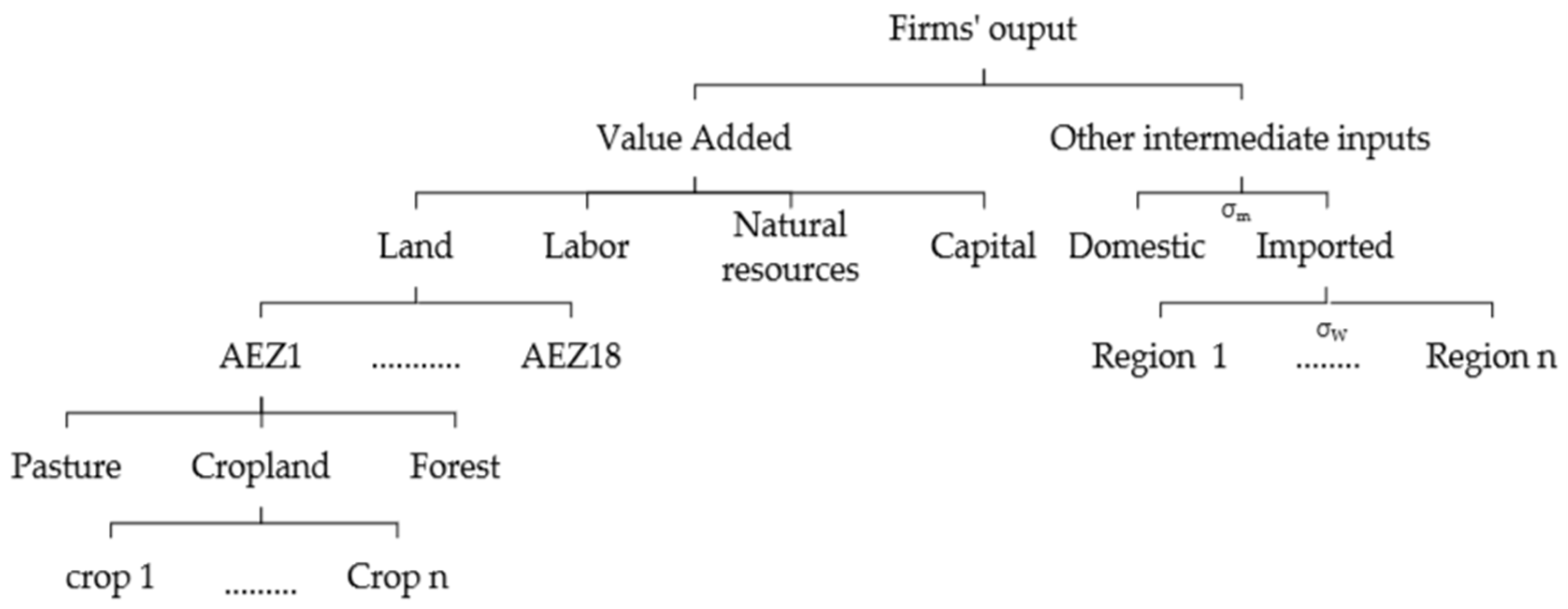
The production technology is represented via nested Constant-Elasticity-of-Substitution (CES) functions that combine primary factors (labor, land, skilled labor, un-skilled labor and natural resources) and intermediate inputs [41].

-

GTAP adopts the Armington assumption in order to differentiate between commodities based on their region of origin [41].

-

It assumes perfect competition, i.e. consumer and producer are price takers, and depict a simultaneous global equilibrium in all regional commodity and factor markets based on endogenous prices [41].

-

A model experiment (shock) perturbs the initial equilibrium and the model is resolved for new market prices for commodities and factors and related supply and demand quantities to clear all markets [41].

-

GTAP is widely used in different types of analyses, now often combined with additional data and related extensions, such as the GTAP-AEZ (Agro-Ecological Zones) [46] for detail in land use and GTAP-Energy [48] for detail in energy products, supply and demand.

GTAP Data

-

The globally consistent GTAP database [42] is constructed based on national accounts and other economic statistics.

-

It represents the world economy in a specific year including complete bilateral trade information and transport margins [42].

-

Its latest version 9 depicts the global economy in 2011 by 140 regions and 57 sectors of which 20 are agri-food sectors [42].

-

Additional data bases cover CO₂ [48] and non-CO₂ emissions [49] relevant for climate changes as well as land cover and use by 18 Agro-Ecological Zones [45,46].

Apart from the structural sensitivity analysis, we conduct an Armington sensitivity analysis as a robustness test to explore the influence of changes in trade elasticities especially with respect to our findings on trade mediated land use leakage effects. Specifically, we assume varying levels of substitutability between imported and domestic commodities, reflected by the Constant Elasticity of Substitution (CES) parameter σ_m (the smaller σ_m, the lower is the substitution among imported and locally produced commodities), and varying levels of substitution of imported commodities by source, reflected by the CES parameter σ_w (See Figure 1).

As usual in global CGE analysis, we aggregate the database, but only regarding regions while maintaining the full GTAP database resolution of 57 production sectors. As regional aggregation can introduce bias in the analysis (cf. Britz et van der Mensbrugghe, [51]), we compare results from two different aggregations with 35 and 70 regions (see

Table A2. Regional aggregation (35 regions).

GTAP Region	Description	GTAP Region	Description
Israel	Israel	Argentina	Argentina
Australia	Australia	Brazil	Brazil
New Zealand	New Zealand	Rest of Latin America	Dominican Republic, Bolivia, Chile, Colombia, Ecuador, Paraguay, Peru, Uruguay, Venezuela, Rest of South America, Costa Rica, Guatemala, Honduras, Nicaragua, Panama, El Salvador, Rest of Central America, Jamaica, Puerto Rico, Trinidad and Tobago, Carib
Rest of Oceania	Rest of Oceania	EU28	Austria, Belgium, Cyprus, Czech Republic, Denmark, Estonia, Finland, France, Germany, Greece, Hungary, Ireland, Italy, Latvia, Lithuania, Luxembourg, Malta, Netherlands, Poland, Portugal, Slovakia, Slovenia, Spain, Sweden, United Kingdom, Bulgaria, Croatia, Romania
China	China	Rest of Europe	Switzerland, Norway, Rest of EFTA, Rest of Europe
Rest of East Asia	Hong Kong, Mongolia, Taiwan, Rest of East Asia	Belarus	Belarus
Rest of South East Asia	Brunei Darussalam, Cambodia, Lao People’s Democratic Republic, Singapore, Thailand, Viet Nam, Rest of Southeast Asia	Former Russian Federation	Albania, Russian Federation, Rest of Eastern Europe, Kazakhstan, Kyrgyzstan, Rest of Former Soviet Union, Armenia, Azerbaijan, Georgia
Rest of South Asia	Bangladesh, Nepal, Pakistan, Sri Lanka, Rest of South Asia	Ukraine	Ukraine
Japan	Japan	other Middle East	Oman, Bahrain, Jordan, Kuwait, Qatar, Saudi Arabia, United Arab Emirates
Korea	Korea	Islamic Republic of Iran	Islamic Republic of Iran
Indonesia	Indonesia	Turkey	Turkey
Malaysia	Malaysia	Rest of Western Asia	Rest of Western Asia
Philippines	Philippines	Mediterranean Africa	Egypt, Morocco, Tunisia, Rest of North Africa
India	India	Nigeria	Nigeria
Canada	Canada	South Africa	South Africa
USA	USA	Rest of Africa	Rest of Africa-
Mexico	Mexico	Rest of the World	Benin, Burkina Faso, Cameroon, Cote d’Ivoire, Ghana, Guinea, Senegal, Togo, Rest of Western Africa, Central Africa, South Central Africa, Ethiopia, Kenya, Madagascar, Malawi, Mauritius, Mozambique, Rwanda, Tanzania, Uganda, Zambia, Zimbabwe, Rest of Eastern Africa, Botswana, Namibia, Rest of South African Customs
Rest of North America	Rest of North America

and

Table A3. Regional aggregation (70 regions).

GTAP Region	Description	GTAP Region	Description
Israel	Israel	Belgium	Belgium
Australia	Australia	Finland	Finland
New Zealand	New Zealand	Sweden	Sweden
Rest of Oceania	Rest of Oceania	Netherlands	Netherlands
China	China	Portugal	Portugal
Taiwan	Taiwan	Ireland	Ireland
Rest of East Asia	Hong Kong, Mongolia, Rest of East Asia, Brunei Darussalam	Denmark	Denmark
Rest of South East Asia	Cambodia, Lao People’s Democratic Republic, Singapore, Rest of Southeast Asia	Austria	Austria
Rest of South Asia	Nepal, Sri Lanka, Rest of South Asia	Greece	Greece
Thailand	Thailand	Luxembourg	Luxembourg
Viet Nam	Viet Nam	Poland	Poland
Pakistan	Pakistan	Hungary	Hungary
Bangladesh	Bangladesh	Slovakia	Slovakia
Japan	Japan	Slovenia	Slovenia
Korea	Korea	Rest of EU 13	Cyprus, Czech Republic, Estonia, Latvia, Lithuania, Malta, Bulgaria, Croatia, Romania
Indonesia	Indonesia	Rest of Europe	Switzerland, Norway, Rest of EFTA, Rest of Europe
Malaysia	Malaysia	Belarus	Belarus
Philippines	Philippines	Former Russia	Albania, Russian Federation, Rest of Eastern Europe, Kazakhstan, Kyrgyzstan, Rest of Former Soviet Union, Armenia, Azerbaijan, Georgia
India	India	Ukraine	Ukraine
Canada	Canada	Gulf	Oman, Bahrain, Jordan, Kuwait, Qatar, United Arab Emirates
USA	USA	Saudi Arabia	Saudi Arabia
Mexico	Mexico	Islamic Republic of Iran	Islamic Republic of Iran
Rest of North America	Rest of North America	Turkey	Turkey
Argentina	Argentina	Rest of Western Asia	Rest of Western Asia
Venezuela	Venezuela	Egypt	Egypt
Peru	Peru	Morocco	Morocco
Colombia	Colombia	Other Mediterranean Africa	Tunisia, Rest of North Africa
Brazil	Brazil	Tanzania	Tanzania
Chile	Chile	Uganda	Uganda
Rest of Latin America	Dominican Republic, Bolivia, Ecuador, Paraguay, Uruguay, Rest of South America, Costa Rica, Guatemala, Honduras, Nicaragua, Panama, El Salvador, Rest of Central America, Jamaica, Puerto Rico, Trinidad and Tobago, Caribbean	Ethiopia	Ethiopia
Germany	Germany	Kenia	Kenia
France	France	Nigeria	Nigeria
UK	UK	South Africa	South Africa
Italy	Italy	Rest of Africa	Benin, Burkina Faso, Cameroon, Cote d’Ivoire, Ghana, Guinea, Senegal, Togo, Rest of Western Africa, Central Africa, South Central Africa, Madagascar, Malawi, Mauritius, Mozambique, Rwanda, Zambia, Zimbabwe, Rest of Eastern Africa, Botswana, Namibia, Rest of South African Customs
Spain	Spain	Rest of the World	Rest of the World

in Appendix A). In the more disaggregated dataset, we increase the representation of the EU28 member states from only one aggregated region (EU28) to 19 countries and one new aggregated region (Rest of EU13), which includes Cyprus, Czech Republic, Estonia, Latvia, Lithuania, Malta, Bulgaria, Croatia, and Romania. This increase in the EU regional representation will allow (1) to consider the heterogeneity between EU28 member states in terms of forest biomass potential, (2) to trace more details and (3) to check the sensitivity of our GTAP simulation results to the level of data aggregation.

2.2. Scenario Design

For our simulation experiment, we assume that the EU28 embarks on a bio-based transformation pathway that involves the partial substitution of non-bio-based inputs for products and services (i.e., intermediate inputs) provided from the forestry sector [11,18], which is described as: Forestry, logging, and related service activities in GTAP9 database. Specifically, we assume a 1% increase in intermediate demand for forest products in all sectors that already use outputs from forestry (see Figure 2). Such a shift in demand patterns could, for example, be the result of changes in production technologies or sourcing preferences including demand for non-traditional biomass uses.

As intermediate demand is an endogenous result in a CGE analysis and cannot be shocked directly, we assume that the technology will change in the medium term, which is reflected by a re-parameterization of the production function. Specifically, we increase the intermediate input coefficients for forestry output in all sectors by 1%. That alone would however imply overall higher intermediate demand in almost any sector, thus overall higher costs. As that is clearly implausible, we decrease all other intermediate input use. We hence assume technological change where forest products would substitute other inputs, without however introducing detailed assumptions exactly what inputs would be replaced. That change in other inputs is defined such that input production costs remain unchanged at given prices. However, prices must change with the updated production function in the closed accounting framework of the CGE. We discuss the resulting structural adjustments in the economy in the result sections.

3. Results

Results are presented in terms of percentage change compared to baseline values. We select key economic and environmental indicators to illustrate the simulated economy-wide effects of increased forest input demand in the EU28 and its sub-regions. Our focus is on land use changes given their importance in environmental sustainability assessments. We also explore impacts on the rest of the world to track indirect effects.

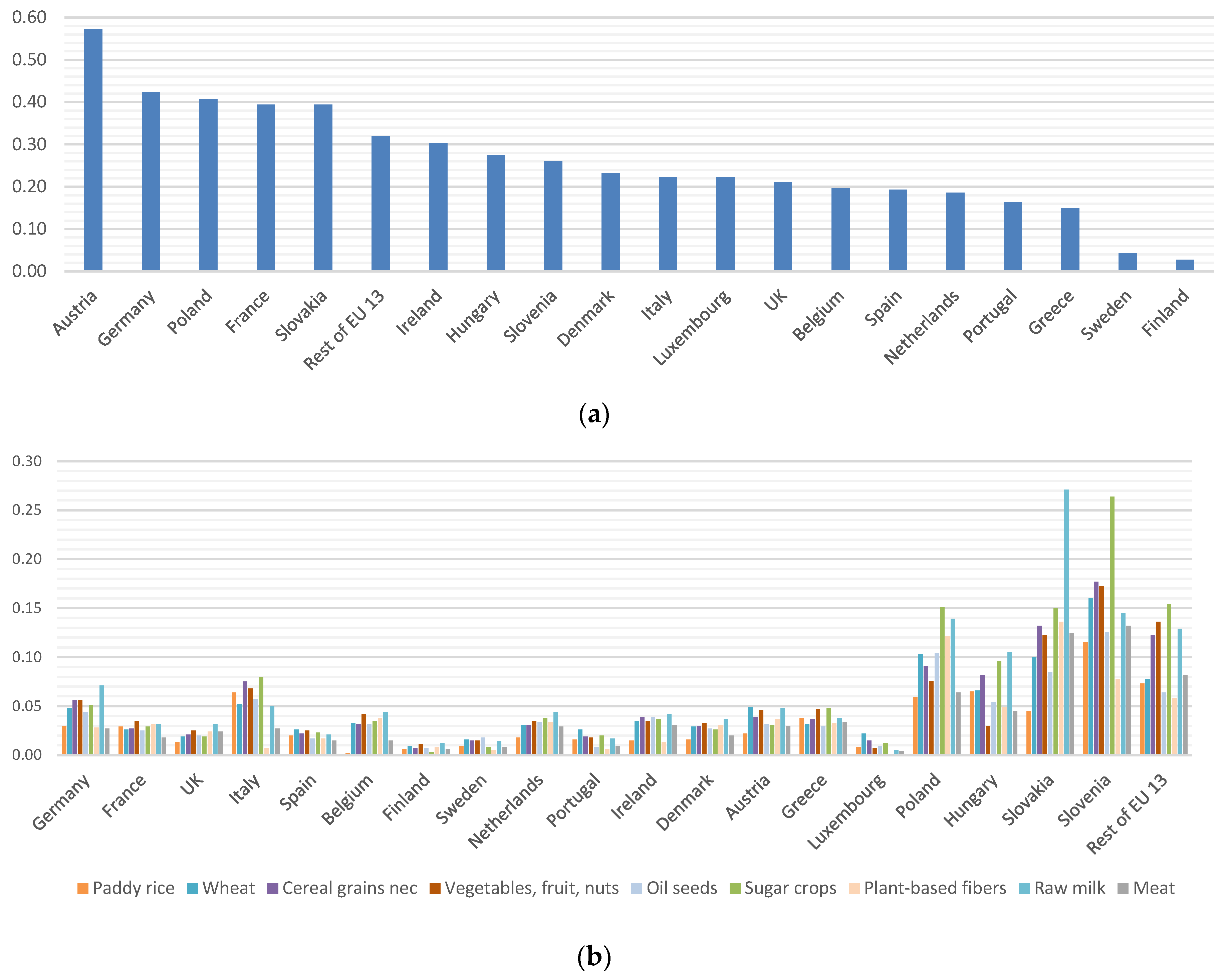
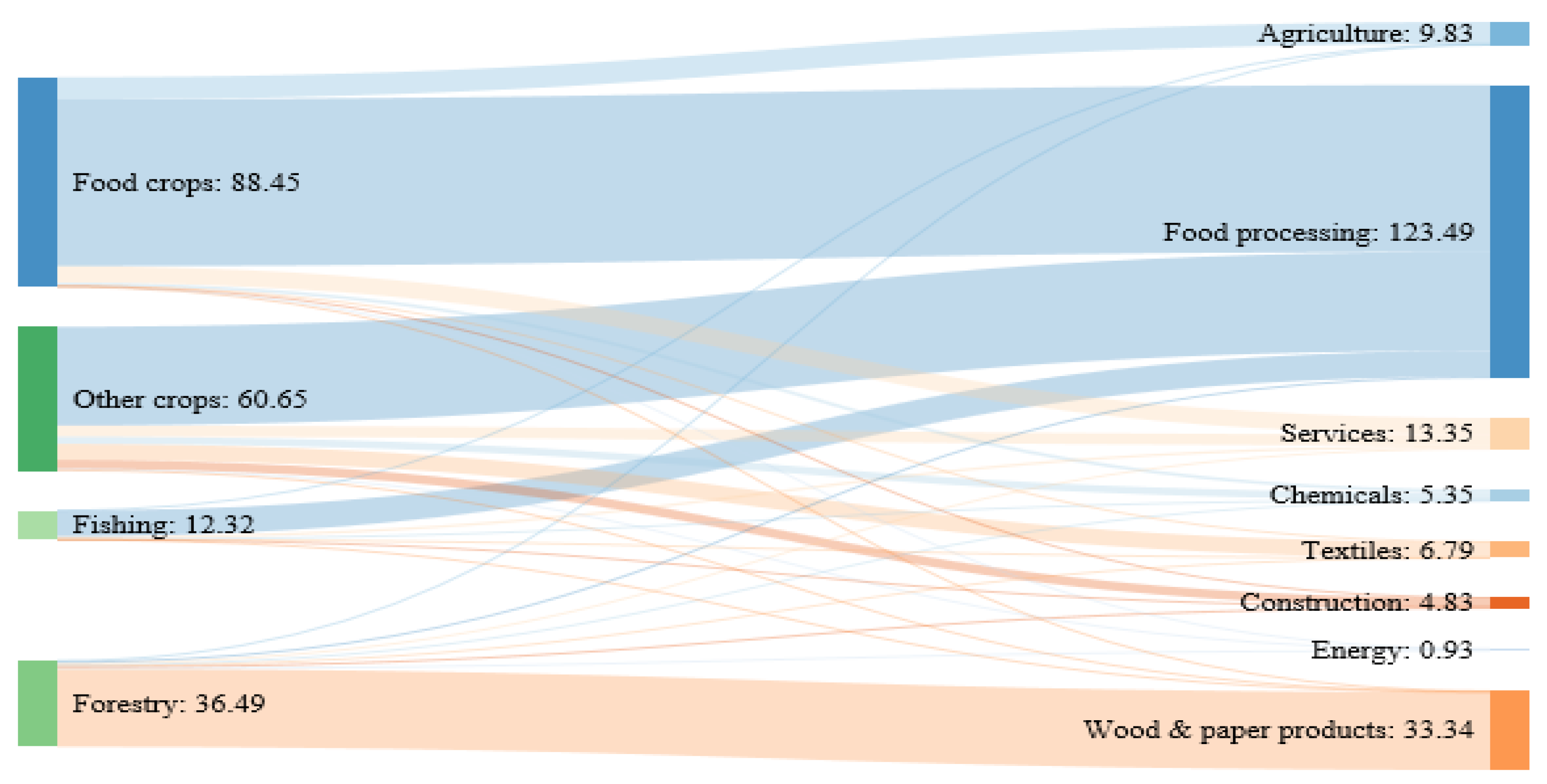
3.1. Effects on Sectoral Output and Prices

Simulation results suggest that a 1% increase in intermediate inputs from the forestry sector to EU28 industries will boost global forestry production by 0.182%. At regional level, Europe exhibits the highest change of 0.82% in the EU28 and 0.21% in the rest of Europe. Forestry production outside Europe is less affected, e.g., in Former Russia and the USA, where forestry production rises by 0.068% and 0.033%, respectively (see

Table 2. Sectoral output changes for selected land-based sectors (%).

Sectors	World	EU28	Rest of Europe	USA	Former Russia	Brazil	Malaysia	Indonesia
Forestry	0.182	0.820	0.210	0.033	0.068	0.010	0.036	0.018
Paddy rice	−0.001	−0.103	−0.052	0.006	−0.001	0.003	−0.004	−0.001
Wheat	−0.001	−0.065	−0.041	0.023	0.019	0.030	0.066	-
Cereal grains	−0.002	−0.030	−0.030	0.003	0.006	0.006	−0.008	−0.001
Oil seeds	−0.002	−0.074	−0.042	0.001	0.008	0.011	−0.006	0.002
Plant-based fibers	−0.003	−0.103	−0.046	0.007	−0.003	−0.004	−0.010	−0.003
Sugar crops	−0.001	−0.008	−0.031	-	−0.002	−0.002	−0.010	−0.001
Raw milk	−0.001	−0.017	−0.011	0.001	−0.003	-	0.001	0.001
Animal products nec 1	−0.003	−0.027	−0.021	0.005	-	0.005	−0.002	-

¹ nec: Not Elsewhere Classified.

below).

According to Table 2, the simulated growth in forest input demand in the EU28 triggers spillover effects on other land-based sectors. Output of all agricultural and food sectors in Europe somewhat shrinks, for example by −0.008% for sugar crops, −0.103% for both paddy rice and plant-based fibers in the EU28, and by −0.011% for raw milk as well as −0.052% for paddy rice in rest of Europe. Indirect effects occur also outside European borders with small effects on agricultural and food sectors in selected world regions. For example, sugar crop production decreases by −0.001% in Indonesia, by −0.002% in both Brazil and Former Russia, and in Malaysia by −0.01%.

These results reflect the reallocation of production factors and intermediate inputs from other economic sectors to forestry. For example, in the EU28, total demand for primary factors in forestry rises by 0.82%, i.e., 0.90% for skilled and un-skilled labor, 0.1% for capital and 0.25% for land. Similarly, total demand for intermediate inputs increases by 1.01%—this includes demand for chemicals, which rises by 0.4%. As a result, we find that countries outside Europe are expected to increase their agricultural output to fill the gap left by dropping EU’s forestry production. In the USA, for example, the output of all agricultural sectors increases and wheat production in particular (+0.023%). These changes in sectoral outputs are driven by market mediated price effects. As the CGE model adjusts prices to balance supply and demand, price changes (see Figure 3) in forestry and agriculture are the underlying mechanisms driving sectoral output.

To meet the higher demand for forest products in the EU28, forestry sectors employ more primary factors (land, capital, labor). This leads to higher factor prices and, thus, production costs and selling prices under the competitive market assumption: the price of forestry output will increase by around 0.3% in the EU28 and at a lower magnitude in rest of Europe (0.06%) and other countries such as the USA (0.01%) and Indonesia (0.02%) (see Figure 3a). The highest primary factor price change is observed in the land market where only forestry and agricultural sectors compete, similarly boosting agricultural output prices (see Figure 3b). In the EU 28, cereal grains suffer the highest price increase (+0.08%) followed by raw milk and paddy rice and vegetables, fruits, and nuts production. Outside the EU28, we find that the agricultural and food markets in Rest of Europe, Former Russia and Ukraine are more affected than in the rest of outside-EU28 countries.

To explore intra-regional differences in impacts of a demand shock of forest products in the EU28, we run the same scenario using a disaggregated database that divides the EU28 into 19 countries and one region (Rest of EU13). The results are consistent with the first experiment.

Table A4. Agricultural and forestry output changes in the EU28 member states (%).

	Forest	Paddy Rice	Wheat	Cereal Grains nec 1	Vegetables, Fruit, Nuts	Oil Seeds	Sugar Crops	Plant-Based Fibers	Crops nec	Animal Products nec	Raw Milk	Meat
Germany	0.83	−0.04	−0.05	−0.03	−0.06	−0.07	−0.02	−0.05	−0.07	−0.05	−0.04	−0.02
France	0.64	−0.06	−0.01	0.01	−0.02	−0.03	−0.00	−0.06	−0.02	−0.00	−0.00	0.00
UK	0.80	0.00	0.01	0.00	−0.01	−0.01	−0.00	−0.06	0.01	−0.01	−0.00	−0.02
Italy	0.78	−0.10	−0.09	−0.02	−0.07	−0.06	−0.00	−0.00	−0.06	−0.01	−0.01	−0.01
Spain	0.87	−0.02	0.01	0.00	0.01	−0.01	−0.00	−0.04	−0.00	0.00	0.00	−0.00
Belgium	0.74	0.12	−0.01	0.00	−0.04	−0.06	−0.00	−0.09	−0.04	0.02	0.01	0.00
Finland	0.06	0.04	0.08	0.03	0.01	0.04	0.01	−0.01	0.02	0.02	0.00	0.00
Sweden	0.11	0.05	0.06	0.02	0.03	0.02	0.00	−0.00	0.01	0.01	0.00	0.01
Netherlands	0.77	−0.00	0.00	−0.00	−0.02	−0.05	−0.01	−0.05	−0.02	−0.00	−0.02	−0.03
Portugal	0.68	−0.01	0.03	0.01	0.01	0.00	0.02	−0.00	0.01	0.01	0.00	0.00
Ireland	0.75	−0.03	−0.04	−0.02	−0.04	−0.09	−0.01	−0.02	−0.01	−0.02	−0.04	−0.03
Denmark	0.74	−0.01	0.02	−0.00	−0.01	−0.02	0.00	−0.05	−0.01	−0.01	−0.01	0.00
Austria	0.54	0.06	−0.03	0.02	−0.01	−0.03	0.03	−0.08	−0.00	−0.03	−0.01	−0.01
Greece	0.57	−0.02	0.02	−0.00	−0.01	−0.01	0.00	−0.08	0.01	−0.02	−0.01	−0.03
Luxembourg	1.05	0.09	0.05	0.03	0.04	0.06	−0.05	0.01	0.06	0.05	0.04	0.00
Poland	0.87	−0.12	−0.10	−0.06	−0.08	−0.11	−0.02	−0.18	−0.15	−0.10	−0.03	−0.04
Hungary	0.90	−0.07	−0.05	−0.03	0.02	−0.07	0.01	−0.12	−0.06	−0.02	−0.01	−0.05
Slovakia	0.87	−0.10	−0.13	−0.11	−0.14	−0.15	−0.02	−0.22	−0.17	−0.07	−0.03	−0.02
Slovenia	0.73	−0.12	−0.26	−0.18	−0.25	−0.37	−0.02	−0.19	−0.28	−0.11	−0.04	−0.01
Rest of EU 13	0.72	−0.13	−0.14	−0.08	−0.09	−0.08	−0.03	−0.09	−0.09	−0.06	−0.04	−0.01

¹ nec: Not Elsewhere Classified.

in Appendix B shows increased forestry output in all EU28 Member States however at different rates, reflecting considerable heterogeneity in forest biomass potential. For example, in Finland and Sweden where forests cover more than three quarters of total land area [23], forestry output rises slightly by 0.06% and 0.11%, respectively. In the rest of EU28, forestry sectors expand more significantly, by +0.54% in Austria, +0.78% in Italy, and over +0.80% in Germany (+0.83%), Poland (+0.87%), and Hungary (+0.90%). Expansion of forestry occurs at the expense of agricultural land in most of the EU countries. For instance, wheat production decreases by −0.26% in Slovenia followed by Rest of EU13 (−0.14%), Slovakia (−0.13%), and Poland (−0.10%). Oil seed production decreases mainly in Slovenia (−0.37%), Slovakia (−0.15%), and Poland (−0.11%).

Price changes in the EU28 differ reflecting the importance of the forestry sector in the land use mix. Forest biomass prices respond most expressively in Austria (+0.58%) followed by Germany (+0.42%), Poland (+0.41%), and France as well as Slovakia (+0.39% in both countries) (see Figure 4a). This also affects agricultural and food markets in all EU28 member states, especially in Poland, Slovakia, and Slovenia (see Figure 4b).

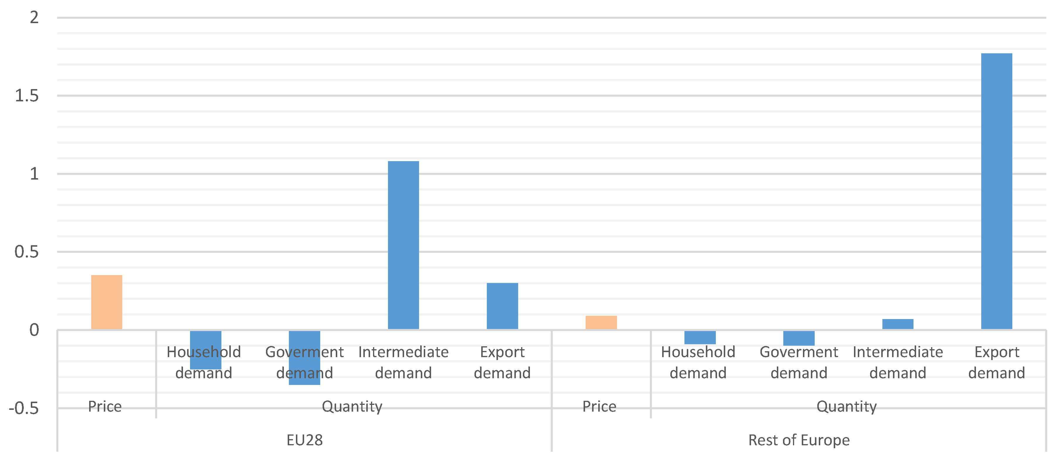
3.2. Effects on Final Demand

In CGE models, final demand is distinguished into four categories, i.e., households, investment, government and export demand [31]. According to the GTAP 9 database, 79% of forest products in the EU28 are used by other downstream industries as intermediate inputs, while the remaining 21% is allocated between the four categories of final demand: 46.6% for households, 48.3% for export demand, around 4.9% for investments, and a negligible share to government final consumption.

As increased intermediate demand for forestry output provokes price increases, household demand for forestry products decrease by −0.03% at a global level. In the EU28, household and government demand decease by −0.25% and −0.35%, respectively. Export demand of forest products increases by 0.3%, nonetheless (see Figure A2 in Appendix B). Countries with abundant forest areas are predicted to increase their exports to the EU28, the rest of European countries in particular (+1.77%), see also next section. Effects on investment demand are negligible.

At regional EU level, our forest-based bioeconomy scenario essentially comes at the price of household consumption as consumer prices rise.

Table 3. Effects on demand (%) for forest products by EU28 member states.

Member States	Price 1	Quantity
		Household Demand	Government Demand	Intermediate Demand	Export Demand
Germany	0.39	−0.33	−0.42	1.16	−0.13
France	0.38	−0.31	−0.39	1.05	−0.5
UK	0.2	−0.16	−0.21	1.06	0.2
Italy	0.22	−0.18	−0.22	1.03	0.66
Spain	0.19	−0.14	−0.19	0.97	0.6
Belgium	0.21	−0.19	−0.2	1.01	0.59
Finland	0.04	−0.03	−0.03	0.02	0.74
Sweden	0.06	−0.06	−0.05	0.02	1.01
Netherlands	0.15	−0.11	−0.19	1.02	0.84
Portugal	0.16	−0.11	−0.17	0.71	0.82
Ireland	0.27	−0.24	−0.3	1.08	0.25
Denmark	0.23	−0.21	−0.23	1.21	0.79
Austria	0.5	−0.44	−0.57	1.01	−0.63
Greece	0.15	−0.11	−0.15	1	0.46
Luxembourg	0.24	−0.24	−0.23	0.89	1.24
Poland	0.39	−0.23	−0.4	1.15	0.34
Hungary	0.27	−0.16	−0.27	1.15	1.08
Slovakia	0.39	−0.25	−0.39	1.08	0.52
Slovenia	0.26	−0.18	−0.26	1.12	1.13
Rest of EU 13	0.32	−0.19	−0.32	0.98	0.12

¹ Average consumer price.

shows that private consumers in Austria will face the most pronounced increase in the prices of forestry products compared to the rest of EU28 countries (+0.5%).

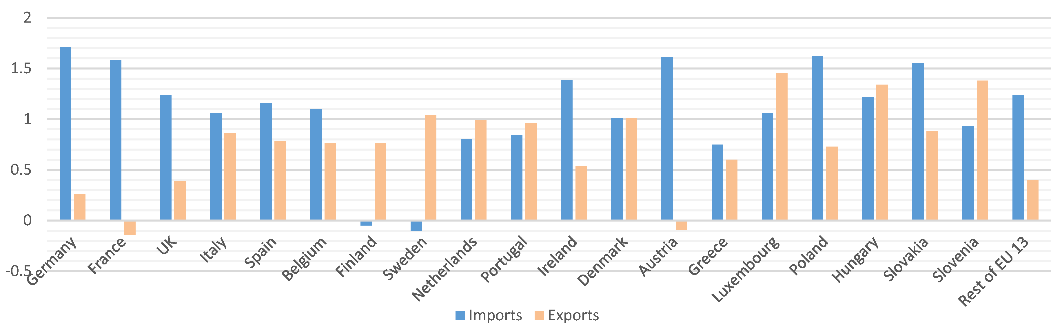
3.3. Effects on Trade Patterns of Forest Products

To meet the additional domestic demand, total EU28 imports of forest products rise by around 1.39%. These imports are mainly coming from the EU28 member states themselves (see

Table 4. Effects on EU 28 trade of forest products by main partner.

	Imports by Country of Origin		Exports by Destination
Sourcing Regions	Baseline ($US Billion)	Scenario (% Change)	Destination Regions	Baseline ($US Billion)	Scenario (% Change)
EU28	4.85	1.02	EU28	5.21	1.00
Indonesia	0.03	2.29	China	0.41	−1.14
Brazil	0.02	2.27	Rest of Europe	0.29	−0.28
Rest of Europe	0.29	1.97	Nigeria	0.23	−0.43
USA	0.24	2.04	Japan	0.02	−1.19
Former Russia	0.37	2.23	India	0.04	−1.17
Ukraine	0.18	1.88	USA	0.10	−1.01
Belarus	0.13	1.89	Former Russia	0.04	−0.84
Total	7.22	1.39	Total	6.62	0.61

). Despite the increased imports of forest products from other countries, such as the USA (+2.04%), Indonesia (+2.29%) and Brazil (+2.27%), the intra-EU28 trade of forest products is still dominant (around 67% of total EU28 imports of forest products are sourced from the domestic market). We find that the growth in forest products imports along with decreasing exports to the rest of the world would exacerbate the deficit of the extra-EU28 trade balance of forest products by around 5%. The EU28 dependency on its own forest products is explained by the low transaction costs and the strong trade integration among the EU countries. In addition, trade in forest products from other countries has been highly restricted by import tariffs and sustainability certification schemes, such as the Forest Law Enforcement, Governance and trade (FLEGT) action plan [52], which requires that only legally harvested wood, especially in the case of tropical wood, is imported to the EU. However, some exogenous model parameters such as the elasticity of substitution between domestic and imported goods, and between imports from different regions, may also affect simulation results. This last point will be further investigated via a sensitivity test in Section 3.5.2.

Figure 5 illustrates the implications of the shock on the EU28 trade of forest products, at country level. We can classify the EU28 countries into three main groups: the first group, which is the largest one, includes member states exhibiting increases in both their imports and exports of forest products (Germany, UK, Italy, Spain, Belgium, Netherlands, Portugal, Ireland, Denmark, Greece, Luxembourg, Poland, Hungary, Slovakia, Slovenia, and rest of EU13); the second group includes countries which would rely more on imported forest products and decrease their exports to the rest of the world (France and Austria); and the third group characterizes countries with abundant forest biomass resources (Finland and Sweden) which will boost their exports to the rest of the EU28.

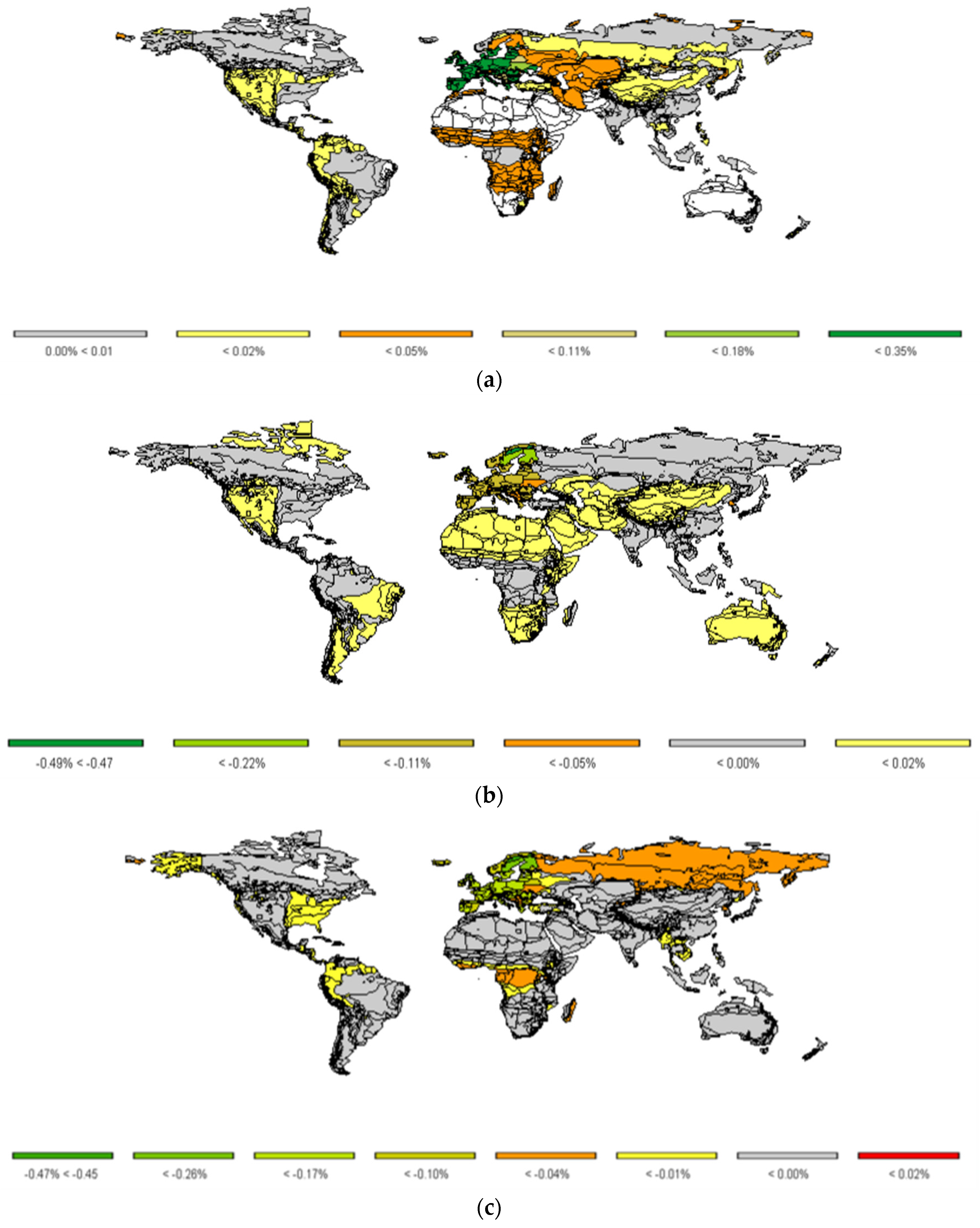
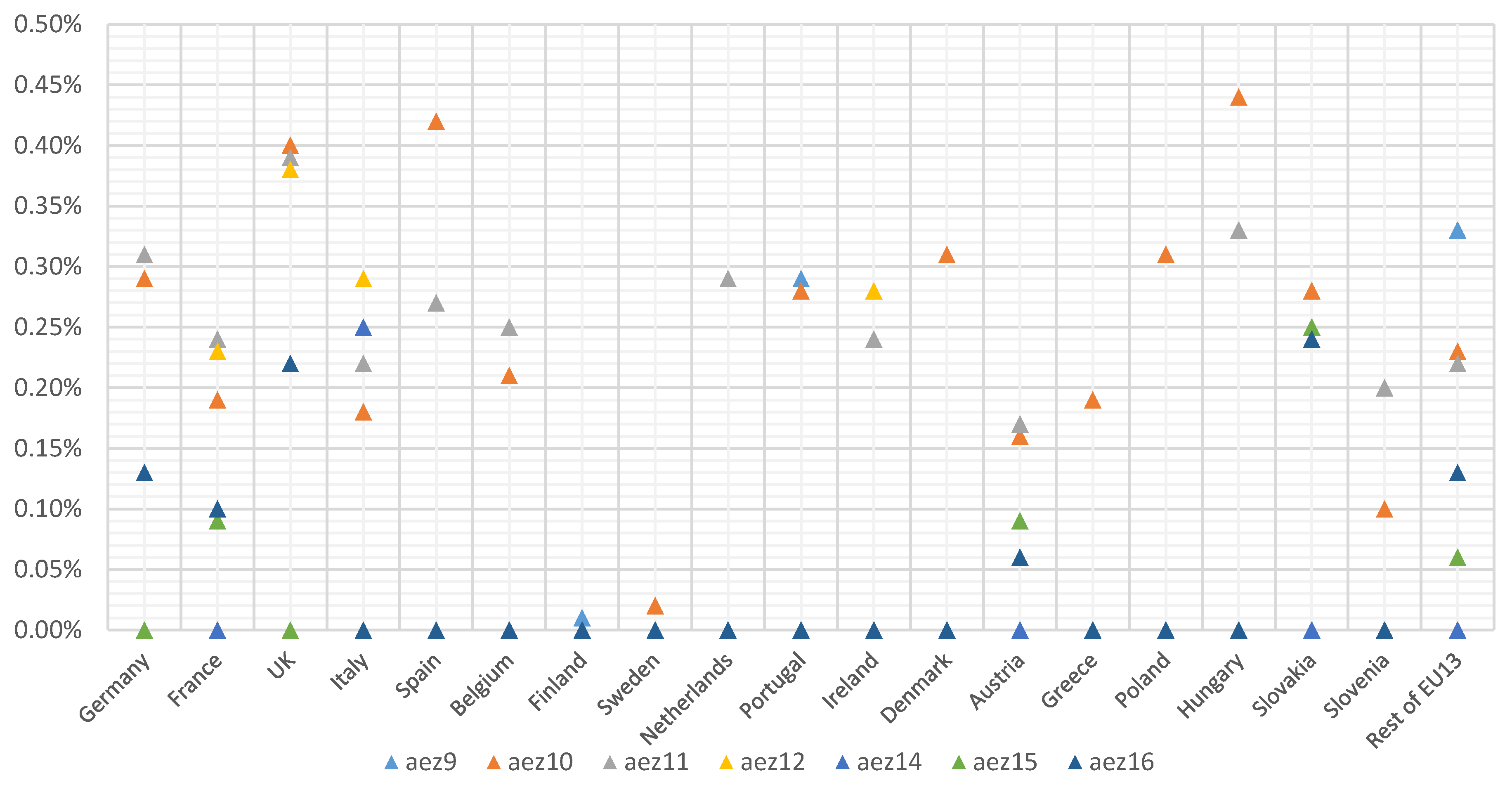
3.4. Effects on LULC Changes

Our forest bioeconomy scenario creates pressure on finite land resources and more competition between its different uses. The maps in Figure 6 show the global percentage change in land area by cover and across all AEZs.

Figure 6a shows that forests expand in all regions. However, the largest impacts are observed in Europe (up to +0.35%) at the expanse of cropland (up to −0.49%) and pasture (up to −0.47%) (Figure 6b,c). This conversion from cropland and pasture to forests reflects increased profitability of the latter due to the rise of forest products prices (see Section 3.1). Outside Europe, the model predicts very low land cover change with scattered impacts in Sub-Saharan Africa, Latin America and Asia, where forests are often converted from pastureland. In fact, cropland increases slightly in all regions (up to +0.02%) while pastureland shows a slight decrease in central Africa and Northern and Western South America. This small indirect effect occurring outside Europe can be mainly explained by the negligible price responsiveness occurring in regions with abundant land resources (see

Table 5. Land use and land rent changes (%).

Regions	Paddy Rice		Wheat		Vegetables, Fruit, Nuts		Oil Seeds		Sugar Crops		Plant-Based Fibers
	Area	Price	Area	Price	Area	Price	Area	Price	Area	Price	Area	Price
EU28	−0.21	0.47	−0.20	0.62	−0.19	0.64	−0.20	0.60	−0.18	0.77	−0.22	0.51
Rest of Europe	−0.09	0.23	−0.09	0.26	−0.08	0.31	−0.09	0.23	−0.08	0.26	−0.10	0.26
Former Russia	−0.01	0.07	−0.01	0.11	−0.01	0.07	−0.01	0.08	−0.01	0.06	−0.01	0.04
Ukraine	−0.02	0.09	−0.06	0.18	−0.06	0.25	−0.04	0.14	−0.06	0.28	−0.07	0.15
Malaysia	−0.01	0.04	0.03	0.26	−0.01	0.04	−0.01	0.04	−0.01	0.03	−0.01	0.02
USA	−0.01	0.07	0.01	0.09	−0.01	0.06	−0.01	0.06	−0.01	0.05	−0.01	0.04
Nigeria	−0.01	0.03	-	0.04	−0.01	0.03	−0.01	0.03	-	0.01	-	-
South Africa	0.01	0.10	0.01	0.10	0.01	0.11	-	0.05	-	0.03	-	0.05
World	−0.01	0.03	−0.03	0.14	−0.02	0.07	−0.02	0.07	−0.01	0.06	−0.02	0.04

).

Figure A3 in Appendix B describes the percentage changes in forestland at detailed EU28 level and by AEZ for the simulation with the disaggregated database (70 regions). Forests expand in all EU28 member states, but at different scales. Finland and Sweden show the lowest increase in their forest area given the already high share of managed forests in these countries [23]. The figure shows also that forest expansion varies across AEZs. We notice that land conversion to forests is mostly seen in AEZ10 (e.g., UK, Spain and Portugal) and in AEZ11 (e.g., Germany, France, and Belgium).

Overall, we can conclude that the increased returns to land in the EU28 forestry sector would rise the area under managed forests and increase the dependency of the EU28 on agricultural and food imports from the rest of the world, even if we only shock the EU28 demand for forest products at the margin. Robustness checks with the disaggregated database (70 regions) produce similar changes at EU and global level. However, regional detail is needed to properly quantify CO₂ emission effects from land use change.

3.5. Sensitivity of Results

In this section, we conduct two different sensitivity experiments: The first one is a structural sensitivity analysis that aims to assess the robustness of the model changes when sectoral production functions and primary factor use are depicted in more detail based on the GTAP-E and GTAP-AGR extensions. The second experiment analyzes the sensitivity of our simulation results with regard to trade elasticities. We select main economic and environmental indicators for comparing results, such as forestry production, trade in forest products, and LULC changes. We also present the GHG emission effects resulting from this marginal change in the EU28 intermediate demand for forest products.

3.5.1. Structural Sensitivity Analysis: GTAP-AEZ-E-AGR Model

Similar to the results from the GTAP Standard plus GTAP-AEZ model, we find that a 1% increase in the intermediate demand for forest inputs lets managed forests expand in all regions, but especially in Europe. However, forestry production in the EU28 rises somewhat stronger by 1.08% once GTAP-E and GTAP-AGR are added, compared to 0.82% in the first experiment. This can be explained by considering substitution in intermediate demand in energy use and in the agricultural and food sectors. This more realistic depiction of production somewhat dampens price effects (more generally, the less flexible production and demand, the higher are price changes and vice versa). At the same time, GTAP-AGR considers that factors are not fully mobile between agricultural and non-agricultural sectors. Compared to the simpler model configuration, this especially dampens increases in forestry production in developing countries with larger primary factor use shares in the agricultural sector. As a consequence of more flexible forest expansion in Europe and less flexible expansion in developing countries, impacts on global trade are dampened. The EU28 imports of forestry products rise by 1.13% compared to 1.39% in the first experiment.

Additionally, the GTAP-E extension allows quantifying changes in the CO₂ emissions only from energy use. Thus, in order to capture effects on total GHG emissions balance, we include data on emissions resulting from LUC based on biomass and soil carbon stock provided by GTAP [50] along with the GTAP non-CO₂ emissions data [49]. Please note that emissions from LUC are amortized linearly, as in Plevin et al. [53] for a selected period of 20 years, following the EU legislation.

As expected,

Table 6. Effects on CO₂ and non-CO₂ greenhouse gas (GHG) emissions in the EU28 (emissions from Land Use Change (LUC) inc.) in teragrams of CO₂ equivalent (Tg CO₂-eq).

GHG Emissions		Baseline	Scenario
CO2		3689.21	3678.67
Non-CO2	N2O	317.01	317.01
	CH4	716.44	716.43
	F GAS 1	158.46	158.47

¹ F GAS: Fluorinated greenhouse gases

shows that afforestation in the EU28 will be accompanied by a decrease in CO₂ emissions of around 10.54 Tg CO₂-eq. However, non-CO₂ emissions remain almost constant.

When exploring changes in the EU28 CO₂ emissions by source, we find that the increased forestry production will be accompanied by using more energy inputs such as coal and oil, resulting in higher CO₂ emissions from fossil fuels combustion (+0.87%). However, the shrinking of other energy-intensive sectors, namely the agricultural sector, would somehow offset this increased pollution and induce a slight positive effect (−0.002%) when looking at the whole EU28 economy. With regards to emissions from LUC, we find that forest expansion mitigates atmospheric emissions (10.54Tg of CO₂-eq at EU28 level) due to increasing soil and biomass carbon stocks. At detailed EU28 level, total GHG emissions are expected to decline in all countries, except for Germany and Greece where emissions would rise by 0.04% and 0.05%, respectively. Ireland, the UK, Sweden, and France exhibit the largest relative decrease in their GHG emissions by −1.33%, −0.24%, −0.17% and −0.15%, respectively.

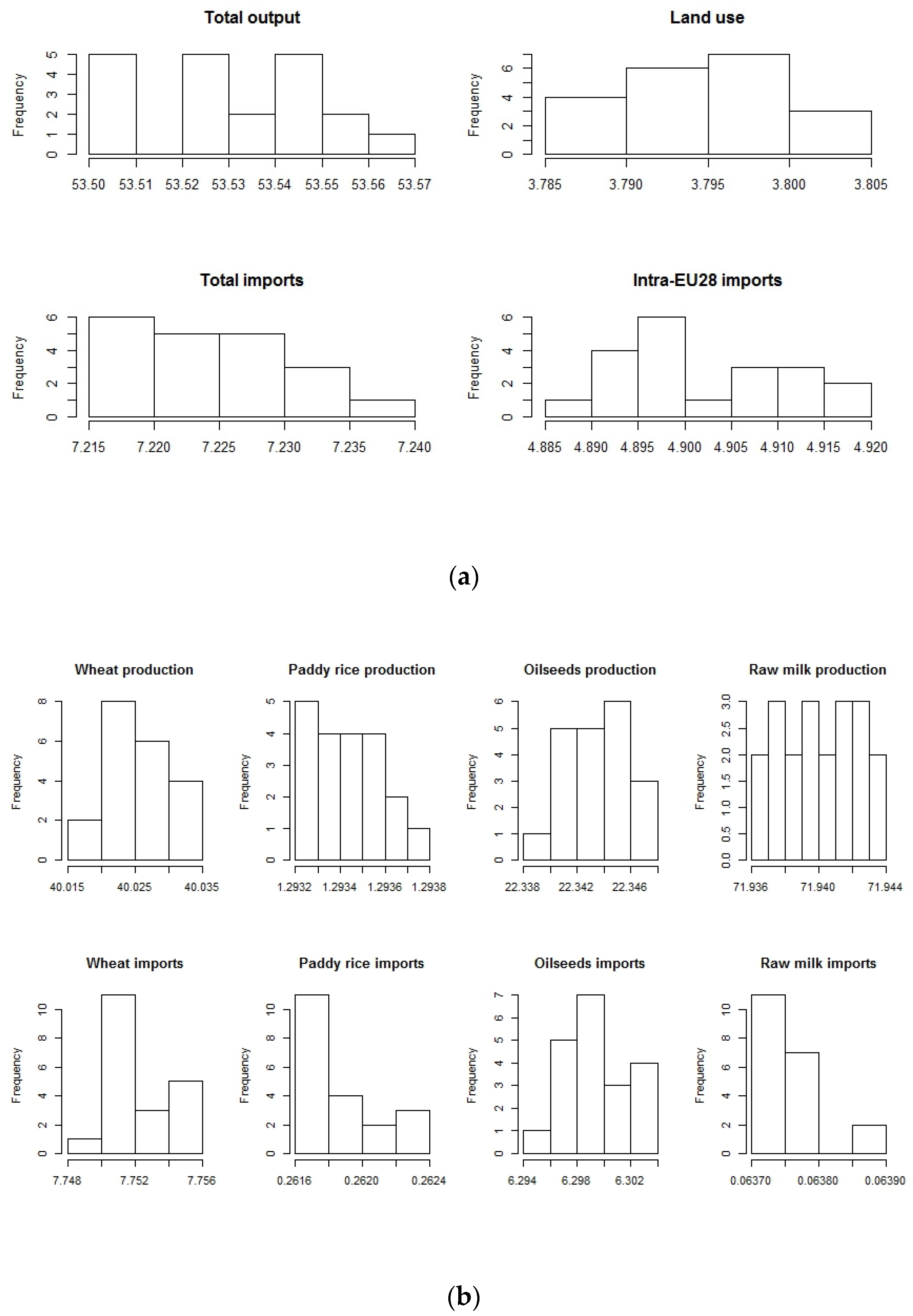
3.5.2. Systematic Sensitivity Analysis

In economic simulation models, results depend heavily on the values of the employed behavioral and other parameters such as price and income elasticities. Therefore, a sensitivity analysis is often undertaken to show how results are affected by those parameters. In this paper, we carry out a multidimensional Systematic Sensitivity Analysis (SSA) on the first level trade elasticity σ_m that reflects the substitution between domestic and foreign commodities in the domestic market and on the second level trade elasticity σ_w that depicts the preferences among commodities which are imported from different trade partners (

Table A5. Default values of first (σ_m) and second level (σ_w) trade elasticities in GTAP9 data for selected land-based sectors.

	σm	σw
Forestry	2.5	5
Wheat	4.45	8.90
Sugar	2.70	5.40
Oil seeds	2.45	4.90
Paddy rice	5.05	10.10
Animal products nec	1.30	2.60
Vegetables, fruit, nuts	1.85	3.70

in Appendix C presents the defaults values of σ_m and σ_w for selected land-based sectors). These trade elasticities are known as the “Armington” elasticities in the literature. To do so, we base our analysis on an integrated Latin Hypercube Sampling (LHS) and an entropy estimator approach. Similar to the Gaussian Quadrature (GQ) approach [54], LHS is often used in large-scale sensitivity analysis. It can be applied with a limited number of simulations, allowing to reduce the computational time. We draw elasticities randomly from a truncated normal distribution in a selected interval (−50%, +50%). The model is solved for N = 20 times. We analyze the obtained results based on the following key variables for the forestry sector: sectoral output, trade, and land use. We use the deviation from the original mean as an indicator for robustness, as used by Schürenberg-Frosch [54].

An overview of results given in

Table 7. Results of the sensitivity analysis for the forestry sector.

Selected Indicators	World			EU28			Rest of Europe
	Original	Mean	Variance	Original	Mean	Variance	Original	Mean	Variance
Sectoral output	284.9731	284.9731	2.67 × 10−6	53.5304	53.5311	3.32 × 10−4	4.4753	4.4753	1.15 × 10−6
Exports	-	-	-	6.1983	6.1987	1.39 × 10−4	0.3372	0.3372	2.15 × 10−7
Imports	-	-	-	7.2243	7.2244	3.2 × 10−5	0.3040	0.3040	1.22 × 10−7
Land use	20.0058	20.0058	1.81 × 10−7	3.7951	3.7953	1.83 × 10−5	0.3120	0.3120	6.47 × 10−8
Selected Indicators	Former Russia			US			Brazil
	Original	Mean	Variance	Original	Mean	Variance	Original	Mean	Variance
Sectoral output	15.3685	15.3685	3.58 × 10−6	22.2379	22.2379	2.67 × 10−6	10.4253	10.4253	5.12 × 10−8
Exports	2.3780	2.3781	2.13 × 10−6	2.6766	2.6766	2.01 × 10−6	0.0522	0.0522	8.84 × 10−9
Imports	0.1112	0.1112	8 × 10−9	0.5318	0.5318	1.85 × 10−8	0.0201	0.0201	1.27 × 10−35
Land use	1.0411	1.0411	2.11 × 10−7	1.4913	1.4913	1.46 × 10−7	0.7256	0.7256	5.16 × 10−9

suggest that the model is robust regarding the trade elasticity parameters. The deviation from the original mean for all selected indicators is rather small for the EU28 and even null for almost all outside-EU28 countries. We also find that intra-EU28 trade on forest products is still dominant; varying the trade elasticities will not result in significant changes, e.g., importing more forest products or deviating from the EU28’s main trade partners. Figure A4 in Appendix C shows the results from the Armington sensitivity analysis in more detail for both forestry and agricultural sectors in the EU28. In the forestry sector, we found that the minimum-maximum spread of the draws is very small (see Figure A4a): it is around +0.13% for forestry production and 0.53% for land use. Same for the agricultural sector, the variation is very small (see Figure A4b). It ranges, for example, between 40.015$ US billion and 40.035$ US billion in wheat production and between 22.338$ US billion and 22.346$ US billion in oilseeds production. Regarding trade, results show that total EU28 imports of forest biomass are barely affected with a remaining dominance of the domestic market. Variation in imports of other agricultural product is also negligible except for oilseed production (+0.16%). Hence, results from the Armington sensitivity analysis can be considered as highly robust.

4. Discussion

The forestry sector has so far been understudied in the literature assessing bio-based transformation scenarios using quantitative models. This paper contributes to fill this gap by highlighting the role, which a forest-based bioeconomy could play in tackling global environmental challenges such as climate change.

Our results suggest that a marginal shift to a more forest-based bioeconomy in the EU28 (+1%) could result in a relatively significant GHG emission abatement of 17.52 Tg of CO₂-eq at global scale. Also, non-EU countries and regions such as Former Russia, Belarus, and the US would decrease their total GHG emissions by around −1.9 Tg CO₂-eq, −0.37 Tg CO₂-eq, −0.63 Tg CO₂-eq, respectively. A forest-based bioeconomy would thus probably be a more effective climate change mitigation strategy than an agriculture-based bioeconomy as far as GHG emissions outcomes are concerned. For example, using an integrated CGE-PE modelling approach, Britz et Hertel [55] found that the EU Biofuels directives are expected to increase global emissions by around 1472 Tg CO₂-eq, due to increased cropland conversion for biodiesel production. In the framework of the European Commission (EC) assessments of the EU 2012 bioeconomy strategy, Domínguez et al. [56] argued that the mitigation potential in agriculture seems to be very modest. Indeed, agricultural GHG emissions are expected to decline by only 2.3% between 2005 and 2030. In opposite to that, a study by Hildebrandt et al. [57] found that the contribution of wood-based construction in Europe alone might allow for a net carbon storage that could reach 46 Tg CO₂-eq per year in 2030. Besides its contribution to climate change mitigation, forests may also play a key role in alleviating the ongoing “Food-Fuel-Material” dilemma [17], which has been driven to a large extent by “First generation” biofuels expansion. Relying more on forest products instead, could reduce pressure on agricultural land. Our results suggest that an increased demand for forestry inputs by the EU28 industries would result in negligible effects on the global agricultural and food markets, e.g., the increase in world crop prices does not exceed +0.02%.

To assess the sensitivity of our results to the aggregation level of the database, we conducted a second experiment using a more disaggregated database (57 sectors and 70 regions). Results are consistent with the findings of the first experiment (57 sectors and 35 regions) but allow to explore regional impacts in more detail. Furthermore, we conducted a structural sensitivity analysis depicting key sectors (energy, agriculture) and their outputs in more detail by adding the GTAP-E and GTAP-AGR extensions. GTAP-E indicates that the transition to a forest-based economy in the EU28 comes with a decrease in total CO₂ emissions. However, non-CO₂ emissions remain constant. Overall, simulation results from different model configuration (GTAP-AEZ, GTAP-AEZ-E, and GTAP-AEZ-E-AGR) are remarkably similar. However, a more detailed description of (1) substitution of different energy sources in production and demand (GTAP-E), (2) in feed use and in the food processing industry as well as considering that factor mobility between agricultural and non-agricultural sectors is limited (GTAP-AGR) overall dampens the global footprint of an increased EU’s reliance on forest products.

Some limitations of this study arise from the used method. The GTAP-AEZ model only considers land under economic uses, i.e., expansion of land uses can only occur through conversion from other managed land uses. This limitation of the GTAP-AEZ model (cf. Golub et al. [58]) could overestimate GHG emission savings as managed forests could also expand into unmanaged ones, while agricultural land cover would decrease less compared to our results. A lower transition from agricultural land and to managed forests implies less GHGs savings. Furthermore, not accounting for changes in natural covers implies as externalities such as loss of natural habitats cannot be accounted for. The accessibility of natural forest, as potential new source of land plays a key role in assessing the sustainability of the growing bioeconomy. For instance, as a result of the increased wood prices and trade openness, natural forests are increasingly degraded in many developing countries due to illegal logging, e.g., tropical forests are declining by around 13 million hectares per year [59]. However, larger increases in forest cover in our study are only found in Europe where natural forests are mostly found in reserves and therefore not subject to land use change such that the limitation of the GTAP-AEZ model is less relevant for our study and the range of changes analyzed.

5. Conclusions

This paper explores the potential impacts of a gradual transition towards a more forest-based European bioeconomy using the standard GTAP CGE model with its extensions (GTAP-AEZ, GTAP-E and GTAP-AGR) and the GTAP 9 database. To do so, we adjust production technologies in the EU28 such that intermediate demand for forest products from all economic sectors increase by 1% and we decrease other intermediate inputs in a cost-neutral way at benchmark prices. Our scenario shows an increased forestry production predominantly in Europe, but also in Brazil, the USA, and Malaysia among others to some extent. As expected, higher demand for forest products increases demand for managed forests, which expands at the expense of cropland and pasture, again mostly in Europe. Increasing the contribution of the forestry sector in the EU bioeconomy may help to reduce GHG emissions and alleviate the potential “food-fuel-Material” tradeoffs associated with non-food uses of agricultural products. Complementary policy action that strengthens the forestry sector may also contribute in achieving the EU’s climate policy targets and thus contribute to unlocking the potential for sustainable transformation in the bioeconomy as proposed in the 2018 update to the European Bioeconomy Strategy. Promising policy measures include regionalized support to technological innovation in wood-based industries, e.g., cascading use of wood and recycling combined with efficient management strategies that enhance forest productivity, targeted at reducing land demand to limit the price effects of a forest-based bioeconomy transition in the EU.

Our study provides first insights into how a European green growth strategy, which fosters an input use of forest products, could play out in terms of global LUC and related GHG emissions. It also highlights the significant role of international trade and land market in mediating and driving impacts from this forest-based bioeconomy transition, at both regional and global scales. However, some caveats of our approach deserve future research efforts. Scenario assumptions could be refined based on current innovation trends and projections to differentiate between changes in intermediate input demand across different GTAP economic sectors. AEZs are still relatively large spatial aggregation units and, thus, land use changes can have very different environmental impacts depending on where within each AEZ they occur. Hence, approaches to spatially disaggregate CGE-based scenario outcomes should be explored along with other techniques to integrate global trade models with life cycle analyses for selected global bioeconomy value chains.

References

1. Dietz, T.; Börner, J.; Förster, J.; von Braun, J. Governance of the bioeconomy: A global comparative study of national bioeconomy strategies. Sustainability 2018, 10, 3190. [Google Scholar] [CrossRef]
2. De Besi, M.; McCormick, K. Towards a Bioeconomy in Europe: National, Regional and Industrial Strategies. Sustainability 2015, 7, 10461–10478. [Google Scholar] [CrossRef] [Green Version]
3. Staffas, L.; Gustavsson, M.; McCormick, K. Strategies and policies for the bioeconomy and bio-based economy: An analysis of official national approaches. Sustainability 2013, 5, 2751–2769. [Google Scholar] [CrossRef]
4. McCormick, K.; Kautto, N. The Bioeconomy in Europe: An Overview. Sustainability 2013, 5, 2589–2608. [Google Scholar] [CrossRef] [Green Version]
5. Wield, D. Bioeconomy and the global economy: Industrial policies and bio-innovation. Technol. Anal. Strateg. Manag. 2013, 25, 1209–1221. [Google Scholar] [CrossRef]
6. Philippidis, G.; M’barek, R.; Ferrari, E. Drivers of the Bioeconomy in Europe towards 2030: Short Overview of an Exploratory, Model-Based Assessment; European Commission, JRC-IPTS: Seville, Spain, 2015. [Google Scholar]
7. European Commission. Life Sciences and Biotechnology: A Strategy for Europe; European Commission: Seville, Spain, 2002. [Google Scholar]
8. European Commission. Taking Sustainable Use of Resources Forward: A Thematic Strategy on the Prevention and Recycling of Waste; European Commission: Seville, Spain, 2005. [Google Scholar]
9. European Commission. Directive 2009/28/EC on the Promotion of the Use of Energy from Renewable Sources and Amending and Subsequently Repealing Directives 2001/77/EC and 2003/30/EC; European Commission: Seville, Spain, 2009. [Google Scholar]
10. European Commission. A Sustainable Bioeconomy for Europe: Strengthening the Connection between Economy, Society and the Environment—Updated Bioeconomy Strategy; European Commission: Seville, Spain, 2018. [Google Scholar]
11. Scarlat, N.; Dallemand, J.-F.; Monforti-Ferrario, F.; Nita, V. The role of biomass and bioenergy in a future bioeconomy: Policies and facts. Environ. Dev. 2015, 15, 3–34. [Google Scholar] [CrossRef] [Green Version]
12. SAT-BBE. Design of a Systems Analysis Tools Framework for a EU Bioeconomy Strategy; Wageningen University & Research: The Hague, The Netherlands, 2015. [Google Scholar]
13. European Commission. Outcome Report on the 2017 Bioeconomy Policy Day; European Commission: Seville, Spain, 2018. [Google Scholar]
14. European Commission. A New EU Forest Strategy: For Forests and the Forest-Based Sector; COM (2013) 659 Final; European Commission: Seville, Spain, 2013. [Google Scholar]
15. Hetemäki, L.; Hanewinkel, M.; Muys, B.; Aho, E. Leading the Way to a European Circular Bioeconomy Strategy; European Forest Institute: Joensuu, Finland, 2017. [Google Scholar]
16. Ollikainen, M. Forestry in bioeconomy—Smart green growth for the humankind. Scand. J. For. Res. 2014, 29, 360–366. [Google Scholar] [CrossRef]
17. Hetemäki, L. Future of the European Forest-Based Sector. Structural Changes towards Bioeconomy; European Forest Institute: Joensuu, Finland, 2014. [Google Scholar]
18. EUSTAFOR. European State Forests Boost the Bioeconomy; Eustafor: Brussels, Belgium, 2017. [Google Scholar]
19. van Leeuwen, M.G.A.; van Meijl, J.C.M.; Smeets, E.M.W. Toolkit for a Systems Analysis Framework of the EU: Overview of WP2 in the EU FP 7 SAT-BBE Project: Systems Analysis Tools Framework for the EU Bio-Based Economy Strategy. Available online: http://edepot.wur.nl/318439 (accessed on 23 January 2017).
20. Philippidis, G.; M’barek, R.; Ferrari, E. Is ‘Bio-Based’ Activity a Panacea for Sustainable Competitive Growth? Energies 2016, 9, 806. [Google Scholar] [CrossRef]
21. European Commission. Forest-Based Industries—Growth—European Commission. Available online: https://ec.europa.eu/growth/sectors/raw-materials/industries/forest-based_en (accessed on 15 October 2018).
22. Forti, R. Agriculture, Forestry and Fishery Statistics; Eurostat: Luxembourg, 2017. [Google Scholar]
23. Hetemäki, L.; Hurmekoski, E. Forest Products Markets under Change: Review and Research Implications. Curr. For. Rep. 2016, 2, 177–188. [Google Scholar] [CrossRef]
24. Wolfslehner, B.; Linser, S.; Pülzl, H. Forest Bioeconomy. A New Scope for Sustainability Indicators; EFI: Joensuu, Spain, 2016. [Google Scholar]
25. Sikkema, R.; Dallemand, J.F.; Matos, C.T.; van der Velde, M.; San-Miguel-Ayanz, J. How can the ambitious goals for the EU’s future bioeconomy be supported by sustainable and efficient wood sourcing practices? Scand. J. For. Res. 2017, 32, 551–558. [Google Scholar] [CrossRef]
26. Hodge, D.; Brukas, V.; Giurca, A. Forests in a bioeconomy: Bridge, boundary or divide? Scand. J. For. Res. 2017, 32, 582–587. [Google Scholar] [CrossRef]
27. Mantau, U.; Saal, U.; Prins, K.; Steierer, F.; Lindner, M.; Yerkerk, H.; Eggers, J.; Leek, N.; Oldenburger, J.; Asikainen, A.; et al. EU Wood: Real Potential for Changes in Growth and Use of EU Forests; Final Report; European Union: Brussels, Belgium, 2010. [Google Scholar]
28. Angenendt, E.; Poganietz, W.-R.; Bos, U.; Wagner, S.; Schippl, J. Modelling and Tools Supporting the Transition to a Bioeconomy. In Bioeconomy: Shaping the Transition to a Sustainable, Biobased Economy; Lewandowski, I., Ed.; Springer: Cham, Switzerland, 2018; pp. 289–316. [Google Scholar]
29. Wicke, B.; van der Hilst, F.; Daioglou, V.; Banse, M.; Beringer, T.; Gerssen-Gondelach, S.; Heijnen, S.; Karssenberg, D.; Laborde, D.; Lippe, M.; et al. Model collaboration for the improved assessment of biomass supply, demand, and impacts. GCB Bioenergy 2015, 7, 422–437. [Google Scholar] [CrossRef]
30. Burfisher, M.E. Introduction to Computable General Equilibrium Models. Available online: https://www.cambridge.org/core/books/introduction-to-computable-general-equilibrium-models/8CE618F19C97979CFC20B3038F2B28F0 (accessed on 15 October 2016).
31. Krey, V.; Havlik, P.; Fricko, O.; Zilliacus, J.; Gidden, M.; Strubegger, M.; Kartasasmita, I.; Ermolieva, T.; Forsell, N.; Gusti, M. Message-Globiom 1.0 Documentation; International Institute for Applied Systems Analysis: Laxenburg, Austria, 2016. [Google Scholar]
32. Banse, M.; van Meijl, H.; Tabeau, A.; Woltjer, G.; Hellmann, F.; Verburg, P.H. Impact of EU biofuel policies on world agricultural production and land use. Biomass Bioenergy 2011, 35, 2385–2390. [Google Scholar] [CrossRef]
33. Smeets, E.; Tabeau, A.; van Berkum, S.; Moorad, J.; van Meijl, H.; Woltjer, G. The impact of the rebound effect of the use of first generation biofuels in the EU on greenhouse gas emissions: A critical review. Renew. Sustain. Energy Rev. 2014, 38, 393–403. [Google Scholar] [CrossRef]
34. Laborde, D. Assessing the Land Use Change Consequences of European Biofuel Policies and Its Uncertainties; Final Report; Prepared by the International Food Policy Institute (IFPRI) for the European Commission: Washington, DC, USA, 2011. [Google Scholar]
35. Britz, W.; Delzeit, R. The impact of German biogas production on European and global agricultural markets, land use and the environment. Energy Policy 2013, 62, 1268–1275. [Google Scholar] [CrossRef]
36. Rosegrant, M.W.; Zhu, T.; Msangi, S.; Sulser, T. Global Scenarios for Biofuels: Impacts and Implications. Available online: https://academic.oup.com/aepp/article/30/3/495/8084 (accessed on 22 January 2017).
37. Havlík, P.; Schneider, U.A.; Schmid, E.; Böttcher, H.; Fritz, S.; Skalský, R.; Aoki, K.; Cara, S.D.; Kindermann, G.; Kraxner, F.; et al. Global land-use implications of first and second generation biofuel targets. Energy Policy 2011, 39, 5690–5702. [Google Scholar] [CrossRef]
38. Wetterlund, E.; Leduc, S.; Dotzauer, E.; Kindermann, G. Optimal use of forest residues in Europe under different policies—Second generation biofuels versus combined heat and power. Biomass Convers. Bioref. 2013, 3, 3–16. [Google Scholar] [CrossRef]
39. Rudi, A.; Müller, A.-K.; Fröhling, M.; Schultmann, F. Biomass Value Chain Design: A Case Study of the Upper Rhine Region. Waste Biomass Valor 2017, 8, 2313–2327. [Google Scholar] [CrossRef]
40. Raumer, H.-G.S.V.; Angenendt, E.; Billen, N.; Jooß, R. Economic and ecological impacts of bioenergy crop production—A modeling approach applied in Southwestern Germany. AIMS Agric. Food 2017, 2, 75–100. [Google Scholar] [CrossRef]
41. Hertel, T.W. Global Trade Analysis: Modeling and Applications; Purdue University: West Lafayette, IN, USA, 1997. [Google Scholar]
42. Aguiar, A.; Narayanan, B.; McDougall, R. An Overview of the GTAP 9 Data Base. J. Glob. Econ. Anal. 2016, 1, 181–208. [Google Scholar] [CrossRef] [Green Version]
43. Britz, W. CGEBox: A Flexible and Modular Toolkit for CGE Modelling with a GUI; University of Bonn: Bonn, Germany, 2018. [Google Scholar]
44. Britz, W.; van der Mensbrugghe, D. CGEBox: A flexible, modular and extendable framework for CGE analysis in GAMS. J. Glob. Econ. Anal. 2018, 3, 106–177. [Google Scholar] [CrossRef]
45. Darwin, R.; Tsigas, M.; Lewandrowski, J.; Raneses, A. World Agriculture and Climate Change Economic Adaptations; Agrcultural Economic Report No. 703; Natural Resource and Environment Division, Economic Research Service, US Department of Agriculture: Washington, DC, USA, 1995.
46. Lee, H.-L.; Hertel, T.; Sohngen, B.; and Ramankutty, N. Towards an Integrated Land Use Data Base for Assessing the Potential for Greenhouse Gas Mitigation; Purdue University: West Lafayette, IN, USA, 2005. [Google Scholar]
47. Keeney, R.; Hertel, T. GTAP-AGR: A Framework for Assessing the Implications of Multilateral Changes in Agricultural Policies; GTAP Technical Papers. Paper 25; Purdue University: West Lafayette, IN, USA, 2005. [Google Scholar]
48. Burniaux, J.-M.; Truong, T.P. GTAP-E: An Energy-Environmental Version of the GTAP Model; GTAP Technical Paper No. 16; Purdue University: West Lafayette, IN, USA, 2002. [Google Scholar]
49. Rose, S.K.; Lee, H.-L. Non-CO2 Greenhouse Gas Emissions Data for Climate Change Economic Analysis; GTAP Working Paper No. 43; Purdue University: West Lafayette, IN, USA, 2008. [Google Scholar]
50. Gibbs, H.; Yui, S.; Plevin, R. New Estimates of Soil and Biomass Carbon Stocks for Global Economic Models; GTAP Technical Paper No. 33; Purdue University: West Lafayette, IN, USA, 2014. [Google Scholar]
51. Britz, W.; van der Mensbrugghe, D. Reducing unwanted consequences of aggregation in large-scale economic models—A systematic empirical evaluation with the GTAP model. Econ. Model. 2016, 59, 463–472. [Google Scholar] [CrossRef]
52. European Commission. Forest Law Enforcement, Governance and Trade (Flegt).com; 251 Final: Proposal for an EU Action Plan; European Commission: Seville, Spain, 2003. [Google Scholar]
53. Plevin, R.J.; Gibbs, H.K.; Duffy, J.; Yui, S.; Yeh, S. Agro-Ecological Zone Emission Factor (AEZ-EF) Model; California Air Resources Board: Sacramento, CA, USA, 2014. [Google Scholar]
54. Schürenberg-Frosch, H. We Could Not Care Less About Armington Elasticities But Should We?: A Meta-Sensitivity Analysis of the Influence of Armington Elasticity Misspecification On Simulation Results. SSRN J. 2015. [Google Scholar] [CrossRef]
55. Britz, W.; Hertel, T.W. Impacts of EU biofuels directives on global markets and EU environmental quality: An integrated PE, global CGE analysis. Agric. Ecosyst. Environ. 2011, 142, 102–109. [Google Scholar] [CrossRef]
56. Domínguez, I.P.; Fellmann, T.; Weiss, F.; Witzke, P.; Barreiro-Hurlé, J.; Himics, M.; Jansson, T.; Salputra, G.; Leip, A. An Economic Assessment of GHG Mitigation Policy Options for EU Agriculture: (EcAMPA 2); JRC Science for Policy Report, EUR 27973 EN, 10.2791/843461; European Commission: Seville, Spain, 2016. [Google Scholar]
57. Hildebrandt, J.; Hagemann, N.; Thrän, D. The contribution of wood-based construction materials for leveraging a low carbon building sector in Europe. Sustain. Cities Soc. 2017, 34, 405–418. [Google Scholar] [CrossRef]
58. Golub, A.; Hertel, T.W.; Brent, S. Land Use Modeling in Recursively-Dynamic GTAP Framework; GTAP Working Paper No. 48; Purdue University: West Lafayette, IN, USA, 2008. [Google Scholar]
59. European Commission. Deforestation: Forests and the Planet’s Biodiversity Are Disappearing. Available online: http://ec.europa.eu/environment/forests/deforestation.htm (accessed on 15 November 2018).
Figure 1. Nested supply function in GTAP plus GTAP-AEZ model. σm is the Constant Elasticity of Substitution (CES) parameter between domestic and imported goods while σw is the Constant Elasticity of Substitution (CES) parameter between goods, which are imported from different regions.
Forests 10 00052 g001
Figure 2. Scenario design.
Forests 10 00052 g002
Figure 3. Price changes (%). (a) Forest biomass. (b) Agricultural and food products.
Forests 10 00052 g003
Figure 4. Price changes in the EU28 (%). (a) Forest products. (b) Agricultural and food products.
Forests 10 00052 g004
Figure 5. Impacts on the EU28 trade of forestry sector products (% change).
Forests 10 00052 g005
Figure 6. Impacts on land cover change (%). (a) Change in Forest cover (%). (b) Change in cropland cover (%). (c) Change in pastureland cover.
Forests 10 00052 g006