Natalie 2.0: Sparse Global Network Alignment as a Special Case of Quadratic Assignment ^†

Abstract

Data on molecular interactions is increasing at a tremendous pace, while the development of solid methods for analyzing this network data is still lagging behind. This holds in particular for the field of comparative network analysis, where one wants to identify commonalities between biological networks. Since biological functionality primarily operates at the network level, there is a clear need for topology-aware comparison methods. We present a method for global network alignment that is fast and robust and can flexibly deal with various scoring schemes taking both node-to-node correspondences as well as network topologies into account. We exploit that network alignment is a special case of the well-studied quadratic assignment problem (QAP). We focus on sparse network alignment, where each node can be mapped only to a typically small subset of nodes in the other network. This corresponds to a QAP instance with a symmetric and sparse weight matrix. We obtain strong upper and lower bounds for the problem by improving a Lagrangian relaxation approach and introduce the open source software tool Natalie 2.0, a publicly available implementation of our method. In an extensive computational study on protein interaction networks for six different species, we find that our new method outperforms alternative established and recent state-of-the-art methods.

1. Introduction

In the last decade, data on molecular interactions has increased at a tremendous pace. For instance, the STRING database [1], which contains protein-protein interaction (PPI) data, grew from 261,033 proteins in 89 organisms in 2003 to 9,643,763 proteins in 2031 organisms in 2015, more than doubling the number of proteins in the database every two and a half years. The same trends can be observed for other types of biological networks, including metabolic, gene-regulatory, signal transduction and metagenomic networks, where the latter can incorporate the excretion and uptake of organic compounds through, for example, a microbial community [2,3]. In addition to the plethora of experimentally derived network data for many species, the structure and behavior of molecular networks have also become intensively studied over the last few years [4], leading to the observation of many conserved features at the network level. However, the development of solid methods for analyzing network data is still lagging behind, particularly in the field of comparative network analysis. Here, one wants to identify commonalities between biological networks from different strains or species, or derived form different conditions. Based on the assumption that evolutionary conservation implies functional significance, comparative approaches may help (i) improve the accuracy of data; (ii) generate, investigate, and validate hypotheses; and (iii) transfer functional annotations. Until recently, the most common way of comparing two networks has been to solely consider node-to-node correspondences, for example by finding homologous relationships between nodes (e.g., proteins in PPI networks) of either network, while the topology of the two networks has not been taken into account. Since biological functionality primarily operates at the network level, there is a clear need for topology-aware comparison methods. In this paper, we present a network alignment method that is fast and robust, and can flexibly deal with various scoring schemes taking both node-to-node correspondences as well as network topologies into account.

1.1. Previous Work

Network alignment establishes node correspondences based on both node-to-node similarities and conserved topological information. Similar to sequence alignment, local network alignment aims at identifying one or more shared subnetworks, whereas global network alignment addresses the overall comparison of the complete input networks. In this paper, we focus on pairwise global network alignment.

Over the last few years, many methods have been proposed for this task. An overview of the recent literature on global network alignment is given in [5]. Here, we shortly list the most important algorithms. The IsoRank algorithm by Singh et al. [6] formulates the global alignment problem as an eigenvalue problem, which preferentially matches nodes with similar neighborhood. Klau [7] presented Natalie, the predecessor of Natalie 2.0, which is described in detail in this paper. The methods are based on an integer linear programming approach solved by Lagrangian relaxation. Kuchaiev et al. [8] presented GRAAL, which matches nodes that share a similar distribution of graphlets. Graphlets are small connected non-isomorphic induced subgraphs. Several variations and improvements of this approach have been published since then. GHOST [9] uses spectral signatures of node neighborhoods in a greedy approach to compute alignments. NETAL [10] is a fast greedy aligner that also takes similar node neighborhoods into account. Another fast method is SPINAL [11], a two-stage approach that combines elements of IsoRank with greedy and improvement heuristics. PISwap [12] is a pure improvement heuristic that is based on 3-OPT exchange moves. HubAlign [13] exploits the assumption that hubs in the networks tend to be topologically more conserved. Therefore, it processes nodes in the order of decreasing degree during the heuristic alignment process. MAGNA++ [14] and its predecessor MAGNA are genetic algorithms that aim at directly optimizing several more recent evaluation measures such as the symmetric substructure score (S3). Optnetalign [15] is a meta-aligner that is able to combine the results of several other methods by means of a multi-objective memetic algorithm. L-GRAAL [16] is the latest member of the GRAAL family of aligners. Similarly to Natalie, L-GRAAL uses Lagrangian relaxation but takes graphlets into account in its scoring function.

1.2. Contribution

We present an algorithm for global network alignment based on an integer linear programming (ILP) formulation. We exploit that network alignment is a special case of the well-studied quadratic assignment problem (QAP). We focus on sparse network alignment, where each node can be mapped only to a typically small subset of nodes in the other network. This corresponds to a QAP instance with a symmetric and sparse weight matrix. We improve upon an existing Lagrangian relaxation approach presented in previous work [7] to obtain strong upper and lower bounds for the problem. We exploit the closeness to QAP and generalize a dual descent method for updating the Lagrangian multipliers to the generalized problem. We have implemented the revised algorithm from scratch as the open source software tool Natalie 2.0. In an extensive computational study on protein interaction networks for six different species, we compare Natalie 2.0 to the two established methods GRAAL and IsoRank as well as to the recent L-GRAAL method, which has been shown to perform very well in recent studies [5,16]. We evaluate the number of conserved edges in terms of edge correctness (EC), induced and symmetric substructure scores (ICS and S3), as well as functional coherence of the modules in terms of gene ontology (GO) annotation. We find that Natalie 2.0 outperforms the alternative methods with respect to several quality measures and running time.

Our software tool Natalie 2.0 as well as all data sets used in this study are publicly available at [17]. Natalie 2.0 can also be run via the NatalieQ [18] web interface at [19].

2. Preliminaries

Given two simple graphs $G_1=(V_1,E_1)$ and $G_2=(V_2,E_2)$, an alignment $a:V_1\rightharpoondown V_2$ is a partial injective function from $V_1$ to $V_2$. As such, we have that an alignment relates every node in $V_1$ to at most one node in $V_2$ and that conversely every node in $V_2$ has at most one counterpart in $V_1$. An alignment is assigned a real-valued score using an additive scoring function s defined as follows:

$$s\left(a\right)=\sum _{v\in V_1}c(v,a\left(v\right))+\sum _{\begin{array}{c}v,w\in V_1\\ v<w\end{array}}w(v,a\left(v\right),w,a\left(w\right))$$

(1)

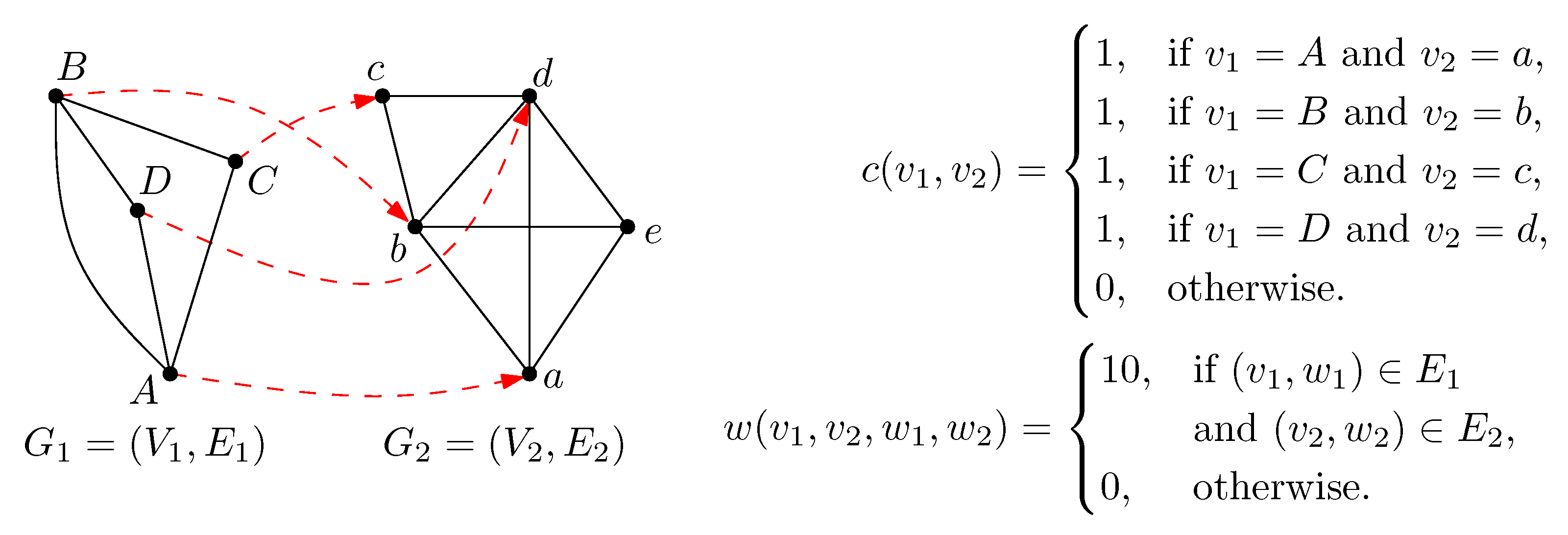
where $c:V_1\times V_2\to \mathbb{R}$ is the score of aligning a pair of nodes in $V_1$ and $V_2$ respectively. On the other hand, $w:V_1\times V_2\times V_1\times V_2\to \mathbb{R}$ allows for scoring topological similarity. The problem of global pairwise network alignment (GNA) is to find the highest scoring alignment $a^{*}=arg\; maxs\left(a\right)$. Figure 1 shows an example:

Figure 1. Example of a network alignment. With the given scoring function, the alignment has a score of $4+40=44$.

Figure 1. Example of a network alignment. With the given scoring function, the alignment has a score of $4+40=44$.

NP-hardness of GNA follows from a simple reduction from the decision problem Clique, which asks whether there is a clique of cardinality at least k in a given simple graph $G=(V,E)$ [20]. The corresponding GNA instance concerns the alignment of the complete graph of k vertices $K_k=(V_k,E_k)$ with G using the scoring function $s\left(a\right)=\left|\right\{(v,w)\in E_k\mid (a\left(v\right),a\left(w\right))\in E\left\}\right|$. Since an alignment is injective, there is a clique of cardinality at least k if and only if the cost of the optimal alignment is $(\genfrac{}{}{0pt}{}{k}{2})$. The close relationship of GNA with the quadratic assignment problem is more easily observed when formulating GNA as a mathematical program. Throughout the remainder of the text, we use variables $i,j\in \{1,\dots ,|V_1\left|\right\}$ and $k,l\in \{1,\dots ,|V_2\left|\right\}$ to denote nodes in $V_1$ and $V_2$, respectively. Let C be a $|V_1|\times |V_2|$ matrix such that $c_{ik}=c(i,k)$ and let W be a $|V_1|\times |V_2|\times |V_1|\times |V_2|$ matrix whose entries $w_{ikjl}$ correspond to interaction scores $w(i,k,j,l)$. Now, we can formulate GNA as

$$\begin{array}{cc}\hfill \underset{x}{max}& \sum _{i,k}{c}_{ik}{x}_{ik}+\sum _{\begin{array}{c}i,j\\ i<j\end{array}}\sum _{\begin{array}{c}k,l\\ k\ne l\end{array}}{w}_{ikjl}{x}_{ik}{x}_{jl}\hfill \end{array}$$

(IQP)

$$\begin{array}{ccc}\hfill \text{s.t.}& \sum _l{x}_{jl}\le 1\hfill & \hfill \forall j\end{array}$$

(2)

$$\begin{array}{ccc}& \sum _j{x}_{jl}\le 1\hfill & \hfill \forall l\end{array}$$

(3)

$$\begin{array}{ccc}& x_{ik}\in \{0,1\}\hfill & \hfill \forall i,k\end{array}$$

(4)

where the decision variable $x_{ik}$ indicates whether the i-th node in $V_1$ is aligned with the k-th node in $V_2$. The above formulation shares many similarities with Lawler’s formulation [21] of the QAP. However, instead of finding an assignment we are interested in finding a matching, which is reflected in Constraints (2) and (3) being inequalities rather than equalities. As can be seen in Equation (1), we only consider the upper triangle of W rather than the entire matrix. An analogous way of looking at this is to consider W to be symmetric. This is usually not the case for QAP instances. In addition, due to the fact that biological input graphs are typically sparse and the restriction of possible matchings to a few candidates per node on average, we have that W is sparse as well. These differences allow us to come up with an effective method of solving the problem as we will see in the following.

3. Methods

The relaxation presented here follows the same lines as the one given by Adams and Johnson for the QAP [22]. We start by linearizing objective function (IQP) by introducing binary variables $y_{ikjl}$ defined as $y_{ikjl}:=x_{ik}·x_{jl}$ and constraints $y_{ikjl}\le x_{jl}$ and $y_{ikjl}\le x_{ik}$ for all $i\le j$ and $k\ne l$. We focus here on the case in which all entries in W are non-negative. Therefore, we do not need to enforce $y_{ikjl}\ge x_{ik}+x_{jl}-1$, which would be necessary in a general linearization of a product of two binary variables. In Section 5, we will discuss this assumption. Rather than using the aforementioned constraints, we make use of a stronger set of constraints which we obtain by multiplying Constraints (2) and (3) by $x_{ik}$:

$$\begin{array}{cc}\hfill \sum _{\begin{array}{c}l\\ l\ne k\end{array}}{y}_{ikjl}=\sum _{\begin{array}{c}l\\ l\ne k\end{array}}{x}_{ik}{x}_{jl}\le \sum _l{x}_{ik}{x}_{jl}\le x_{ik},& \forall i,j,k,i<j\hfill \end{array}$$

(5)

$$\begin{array}{cc}\hfill \sum _{\begin{array}{c}j\\ j>i\end{array}}{y}_{ikjl}=\sum _{\begin{array}{c}j\\ j>i\end{array}}{x}_{ik}{x}_{jl}\le \sum _j{x}_{ik}{x}_{jl}\le x_{ik},& \forall i,k,l,k\ne l\hfill \end{array}$$

(6)

We proceed by splitting the variable $y_{ikjl}$ (where $i<j$ and $k\ne l$). In other words, we extend the objective function such that the counterpart of $y_{ikjl}$ becomes $y_{jlik}$. This is accomplished by rewriting the dummy constraint in Equation (6) to $j\ne i$. In addition, we split the weights: $w_{ikjl}=w_{jlik}=(w_{ikjl}^{\prime }/2)$ where $w_{ikjl}^{\prime }$ denotes the original weight. Furthermore, we require that the counterparts of the split decision variables assume the same value, which results in the following integer linear programming formulation:

$$\begin{array}{cc}\hfill \underset{x,y}{max}& \sum _{i,k}{c}_{ik}{x}_{ik}+\sum _{\begin{array}{c}i,j\\ i<j\end{array}}\sum _{\begin{array}{c}k,l\\ k\ne l\end{array}}{w}_{ikjl}{y}_{ikjl}+\sum _{\begin{array}{c}i,j\\ i>j\end{array}}\sum _{\begin{array}{c}k,l\\ k\ne l\end{array}}{w}_{ikjl}{y}_{ikjl}\hfill \end{array}$$

(ILP)

$$\begin{array}{ccc}\hfill \text{s.t.}& \sum _l{x}_{jl}\le 1\hfill & \hfill \forall j\end{array}$$

(7)

$$\begin{array}{ccc}& \sum _j{x}_{jl}\le 1\hfill & \hfill \forall l\end{array}$$

(8)

$$\begin{array}{ccc}& \sum _{\begin{array}{c}l\\ l\ne k\end{array}}{y}_{ikjl}\le x_{ik}\hfill & \hfill \forall i,j,k,i\ne j\end{array}$$

(9)

$$\begin{array}{ccc}& \sum _{\begin{array}{c}j\\ j\ne i\end{array}}{y}_{ikjl}\le x_{ik}\hfill & \hfill \forall i,k,l,k\ne l\end{array}$$

(10)

$$\begin{array}{ccc}& y_{ikjl}=y_{jlik}\hfill & \hfill \forall i,j,k,l,i<j,k\ne l\end{array}$$

(11)

$$\begin{array}{ccc}& y_{ikjl}\in \{0,1\}\hfill & \hfill \forall i,j,k,l,i\ne j,k\ne l\end{array}$$

(12)

$$\begin{array}{ccc}& x_{ik}\in \{0,1\}\hfill & \hfill \forall i,k\end{array}$$

(13)

We can solve the continuous relaxation of Equation (ILP) via its Lagrangian dual by dualizing the linking constraints Equation (11) with multiplier λ:

$$\begin{array}{cc}\hfill \underset{\lambda }{min}& Z_{\text{LD}}\left(\lambda \right)\hfill \end{array}$$

(LD)

where $Z_{\text{LD}}\left(\lambda \right)$ equals

$$\begin{array}{cc}\hfill & \underset{x,y}{max}\sum _{i,k}{c}_{ik}{x}_{ik}+\sum _{\begin{array}{c}i,j\\ i<j\end{array}}\sum _{\begin{array}{c}k,l\\ k\ne l\end{array}}(w_{ikjl}+{\lambda }_{ikjl})y_{ikjl}+\sum _{\begin{array}{c}i,j\\ i>j\end{array}}\sum _{\begin{array}{c}k,l\\ k\ne l\end{array}}(w_{ikjl}-{\lambda }_{jlik})y_{ikjl}\hfill \\ \hfill & \text{s.t.}\text{Constraints (7)–(13)}\hfill \end{array}$$

Now that the linking constraints have been dualized, one can observe that the remaining constraints decompose the variables into $|V_1\left|\right|V_2|$ disjoint groups, where variables across groups are not linked by any constraint, and where each group contains a variable $x_{ik}$ and variables $y_{ikjl}$ for $j\ne i$ and $l\ne k$. Hence, we have

$$\begin{array}{cc}\hfill Z_{\text{LD}}\left(\lambda \right)=\underset{x}{max}& \sum _{i,k}[c_{ik}+v_{ik}\left(\lambda \right)]x_{ik}\hfill \end{array}$$

(LD_λ)

$$\begin{array}{ccc}\hfill \text{s.t.}& \sum _l{x}_{jl}\le 1\hfill & \hfill \forall j\end{array}$$

(14)

$$\begin{array}{ccc}& \sum _j{x}_{jl}\le 1\hfill & \hfill \forall l\end{array}$$

(15)

$$\begin{array}{ccc}& x_{ik}\in \{0,1\}\hfill & \hfill \forall i,k\end{array}$$

(16)

which corresponds to a maximum weight bipartite matching problem on the so-called alignment graph $G_m=(V_1\cup V_2,E_m)$. In the general case, $G_m$ is a complete bipartite graph, i.e. $E_m=\{(i,k)\mid i\in V_1,v_2\in V_2\}$. However, by exploiting biological knowledge, one can make $G_m$ more sparse by excluding biologically-unlikely edges (see Section 4). For the global problem, the weight of a matching edge $(i,k)$ is set to $c_{ik}+v_{ik}\left(\lambda \right)$, where the latter term is computed as

$$\begin{array}{cc}\hfill v_{ik}\left(\lambda \right)=\underset{y}{max}& \sum _{\begin{array}{c}j\\ j>i\end{array}}\sum _{\begin{array}{c}l\\ l\ne k\end{array}}(w_{ikjl}+{\lambda }_{ikjl})y_{ikjl}+\sum _{\begin{array}{c}j\\ j<i\end{array}}\sum _{\begin{array}{c}l\\ l\ne k\end{array}}(w_{ikjl}-{\lambda }_{jlik})y_{ikjl}\hfill \end{array}$$

(L${\text{D}}_{\lambda }^{ik}$)

$$\begin{array}{ccc}\hfill \text{s.t.}& \sum _{\begin{array}{c}l\\ l\ne k\end{array}}{y}_{ikjl}\le 1\hfill & \hfill \forall j,j\ne i\end{array}$$

(17)

$$\begin{array}{ccc}& \sum _{\begin{array}{c}j\\ j\ne i\end{array}}{y}_{ikjl}\le 1\hfill & \hfill \forall l,l\ne k\end{array}$$

(18)

$$\begin{array}{ccc}& y_{ikjl}\in \{0,1\}\hfill & \hfill \forall j,l\end{array}$$

(19)

Again, this is a maximum weight bipartite matching problem on the same alignment graph but excluding edges incident to either i or k and using different edge weights: the weight of an edge $(j,l)$ is $w_{ikjl}+{\lambda }_{ikjl}$ if $j>i$, or $w_{ikjl}-{\lambda }_{jlik}$ if $j<i$. So, in order to compute $Z_{\text{LD}}\left(\lambda \right)$, we need to solve a total number of $|V_1\left|\right|V_2|+1$ maximum weight bipartite matching problems, which, using the Hungarian algorithm [23,24] can be done in $O\left(n^5\right)$ time, where $n=max\left(\right|V_1|,|V_2\left|\right)$. In case the alignment graph is sparse, i.e., $O\left(\right|E_m\left|\right)=O\left(n\right)$, $Z_{\text{LD}}\left(\lambda \right)$ can be computed in $O(n^{4}logn)$ time using the successive shortest path variant of the Hungarian algorithm [25]. It is important to note that for any λ, $Z_{\text{LD}}\left(\lambda \right)$ is an upper bound on the score of an optimal alignment. This is because any alignment a is feasible to $Z_{\text{LD}}\left(\lambda \right)$ and does not violate the original linking constraints and therefore has an objective value equal to $s\left(a\right)$. In particular, the optimal alignment $a^{*}$ is also feasible to $Z_{\text{LD}}\left(\lambda \right)$ and hence $a^{*}\le Z_{\text{LD}}\left(\lambda \right)$. Since the two sets of problems resulting from the decomposition both have the integrality property [26], the smallest upper bound we can achieve equals the linear programming (LP) bound of the continuous relaxation of Formulation (ILP) [27]. Given solution $(x,y)$ to $Z_{\text{LD}}\left(\lambda \right)$, we obtain a lower bound on $s\left(a^{*}\right)$, denoted $Z_{\text{lb}}\left(\lambda \right)$, by considering the score of the alignment encoded in x.

3.1. Solving Strategies

In this section we will discuss strategies for identifying Lagrangian multipliers λ that yield an as small as possible gap between the upper and lower bound resulting from the solution to $Z_{\text{LD}}\left(\lambda \right)$.

3.1.1. Subgradient Optimization

We start by discussing subgradient optimization, which is originally due to Held and Karp [28]. The idea is to generate a sequence ${\lambda }^0,{\lambda }^1,\dots$ of Lagrangian multiplier vectors starting from ${\lambda }^0=\mathbf{0}$ as follows:

$$\begin{array}{cc}\hfill {\lambda }_{ikjl}^{t+1}={\lambda }_{ikjl}^t-\frac{\alpha ·(Z_{\text{LD}}\left(\lambda \right)-Z_{\text{lb}}\left(\lambda \right))}{\parallel g\left({\lambda }^t\right){\parallel }^2}g({\lambda }_{ikjl}^t)& \forall i,j,k,l,i<j,k\ne l\hfill \end{array}$$

(20)

where $g({\lambda }_{ikjl}^t)$ corresponds to the subgradient of multiplier ${\lambda }_{ikjl}^t$, i.e. $g({\lambda }_{ikjl}^t)=y_{ikjl}-y_{jlik}$, and α is the step size parameter. Initially, α is set to 1 and it is halved if neither $Z_{\text{LD}}\left(\lambda \right)$ nor $Z_{\text{lb}}\left(\lambda \right)$ have improved for over N consecutive iterations. Conversely, α is doubled if M times in a row there was an improvement in either $Z_{\text{LD}}\left(\lambda \right)$ or $Z_{\text{lb}}\left(\lambda \right)$ [29]. In case all subgradients are zero, the optimal solution has been found and the scheme terminates. Note that this is not guaranteed to happen. Therefore, we abort the scheme after exceeding a time limit or a pre-specified number of iterations. In addition, we terminate if α has dropped below machine precision. Algorithm 1 gives the pseudo code of this procedure.

Algorithm 1: SubgradientOpt$(\lambda ,M,N)$

$\alpha \leftarrow 1$; $n\leftarrow N$; $m\leftarrow M$ $[{\text{LB}}^{*},{\mathrm{UB}}^{*}]\leftarrow [Z_{\text{lb}}\left(\lambda \right),Z_{\text{LD}}\left(\lambda \right)]$ while $g\left(\lambda \right)\ne 0$ do  $\lambda \leftarrow \lambda -\frac{\alpha (Z_{\text{LD}}\left(\lambda \right)-Z_{\text{lb}}\left(\lambda \right))}{\parallel g\left({\lambda }^t\right){\parallel }^2}g\left({\lambda }^t\right)$  if $[{\text{LB}}^{*},{\mathrm{UB}}^{*}]\setminus [Z_{\text{lb}}\left(\lambda \right),Z_{\text{LD}}\left(\lambda \right)]=\varnothing$ then $n\leftarrow n-1$  else   ${\text{LB}}^{*}\leftarrow max[{\text{LB}}^{*},Z_{\text{lb}}\left(\lambda \right)]$   ${\mathrm{UB}}^{*}\leftarrow min[{\mathrm{UB}}^{*},Z_{\text{LD}}\left(\lambda \right)]$   $m\leftarrow m-1$  if $n=0$ then $\alpha \leftarrow \alpha /2$$n\leftarrow N$  if $m=0$ then $\alpha \leftarrow 2\alpha$$m\leftarrow M$ return $[{\text{LB}}^{*},{\mathrm{UB}}^{*}]$

3.1.2. Dual Descent

In this section we derive a dual descent method which is an extension of the one presented in [22]. The dual descent method takes as a starting point the dual of $Z_{\text{LD}}\left(\lambda \right)$:

$$\begin{array}{cc}\hfill Z_{\text{LD}}\left(\lambda \right)=\underset{\alpha ,\beta }{min}& \sum _i{\alpha }_i+\sum _k{\beta }_k\hfill \end{array}$$

(21)

$$\begin{array}{ccc}\hfill \text{s.t.}& {\alpha }_i+{\beta }_k\ge c_{ik}+v_{ik}\left(\lambda \right)\hfill & \hfill \forall i,k\end{array}$$

(22)

$$\begin{array}{ccc}& {\alpha }_i\ge 0\hfill & \hfill \forall i\end{array}$$

(23)

$$\begin{array}{ccc}& {\beta }_k\ge 0\hfill & \hfill \forall k\end{array}$$

(24)

where the dual of $v_{ik}\left(\lambda \right)$ is

$$\begin{array}{cc}\hfill v_{ik}\left(\lambda \right)=\underset{\mu ,\nu }{min}& \sum _{\begin{array}{c}j\\ j\ne i\end{array}}{\mu }_j^{ik}+\sum _{\begin{array}{c}l\\ l\ne k\end{array}}{\nu }_l^{ik}\hfill \end{array}$$

(25)

$$\begin{array}{ccc}\hfill \text{s.t.}& {\mu }_j^{ik}+{\nu }_l^{ik}\ge w_{ikjl}+{\lambda }_{ikjl}\hfill & \hfill \forall j,l,j>i,l\ne k\end{array}$$

(26)

$$\begin{array}{ccc}& {\mu }_j^{ik}+{\nu }_l^{ik}\ge w_{ikjl}-{\lambda }_{jlik}\hfill & \hfill \forall j,l,j<i,l\ne k\end{array}$$

(27)

$$\begin{array}{ccc}& {\mu }_j^{ik}\ge 0\hfill & \hfill \forall j\end{array}$$

(28)

$$\begin{array}{ccc}& {\nu }_l^{ik}\ge 0\hfill & \hfill \forall l\end{array}$$

(29)

Suppose that for a given ${\lambda }^t$ we have computed dual variables $(\alpha ,\beta )$ solving Problem (21) with objective value $Z_{\text{LD}}\left({\lambda }^t\right)$, as well as dual variables $({\mu }^{ik},{\nu }^{ik})$ yielding values $v_{ik}\left(\lambda \right)$ to Problems (25). The goal now is to find ${\lambda }^{t+1}$ such that the resulting bound is better or just as good, i.e. $Z_{\text{LD}}\left({\lambda }^{t+1}\right)\le Z_{\text{LD}}\left({\lambda }^t\right)$. We prevent the bound from increasing, by ensuring that the dual variables $(\alpha ,\beta )$ remain feasible for Problem (21). This we can achieve by considering the slacks: ${\pi }_{ik}\left(\lambda \right)={\alpha }_i+{\beta }_k-c_{ik}-v_{ik}\left(\lambda \right)$. Thus, for $(\alpha ,\beta )$ to remain feasible, we can only allow every $v_{ik}\left({\lambda }^t\right)$ to increase by as much as ${\pi }_{ik}\left({\lambda }^t\right)$. We can achieve such an increase by considering Linear Programs (25) and their slacks defined as

$$\begin{array}{ccc}\hfill {\gamma }_{ikjl}\left(\lambda \right)& =\left\{\begin{array}{cc}{\mu }_j^{ik}+{\nu }_l^{ik}-w_{ikjl}+{\lambda }_{ikjl},\hfill & \text{if}j>i,\hfill \\ {\mu }_j^{ik}+{\nu }_l^{ik}-w_{ikjl}-{\lambda }_{jlik},\hfill & \text{if}j<i,\hfill \end{array}\right.\hfill & \hfill \forall j,l,j\ne i,l\ne k\end{array}$$

(30)

and update the multipliers in the following way.

Lemma 1. 

The adjustment scheme below yields solutions to Linear Programs (25) with objective values $v_{ik}\left({\lambda }^{t+1}\right)$ at most ${\pi }_{ik}\left({\lambda }^t\right)+v_{ik}\left({\lambda }^t\right)$ for all $i,k$.

$$\begin{array}{cc}\hfill {\lambda }_{ikjl}^{t+1}={\lambda }_{ikjl}^t& +{\phi }_{ikjl}\left[{\gamma }_{ikjl}\left({\lambda }^t\right)+{\tau }_{ik}\left(\frac{1}{2(n_1-1)}+\frac{1}{2(n_2-1)}\right){\pi }_{ik}\left({\lambda }^t\right)\right]\hfill \\ & -{\phi }_{jlik}\left[{\gamma }_{jlik}\left({\lambda }^t\right)+{\tau }_{jl}\left(\frac{1}{2(n_1-1)}+\frac{1}{2(n_2-1)}\right){\pi }_{jl}\left({\lambda }^t\right)\right]\hfill \end{array}$$

(31)

for all $j,l,i<j,k\ne l$, where $n_1=\left|V_1\right|$, $n_2=\left|V_2\right|$, and $0\le {\phi }_{ikjl},{\tau }_{jl}\le 1$ are parameters.

Proof. 

We prove the lemma by showing that for any $i,k$ there exists a feasible solution $({\mu }^{\prime ik},{\nu }^{\prime ik})$ to Problem (25) whose objective value $v_{ik}\left({\lambda }^{t+1}\right)$ is at most ${\pi }_{ik}\left({\lambda }^t\right)+v_{ik}\left({\lambda }^t\right)$. Let $({\mu }^{ik},{\nu }^{ik})$ be the solution to Problem (25) given multipliers ${\lambda }^t$. We claim that setting

$$\begin{array}{cc}\hfill {\mu }_j^{\prime ik}={\mu }_j^{ik}+\frac{{\pi }_{ik}\left({\lambda }^t\right)}{2(n_1-1)}& \forall j,j\ne i\hfill \\ \hfill {\nu }_l^{\prime ik}={\nu }_j^{ik}+\frac{{\pi }_{ik}\left({\lambda }^t\right)}{2(n_2-1)}& \forall l,l\ne k\hfill \end{array}$$

results in a feasible solution to Problem (25) given multipliers ${\lambda }^{t+1}$. We start by showing that Constraints (26) and (27) are satisfied. Equation (31) implies the following bounds on ${\lambda }^{t+1}$:

$$\begin{array}{cc}\hfill {\lambda }_{ikjl}^t-{\gamma }_{jlik}\left({\lambda }^t\right)-\left(\frac{1}{2(n_1-1)}+\frac{1}{2(n_2-1)}\right){\pi }_{jl}\left({\lambda }^t\right)\le {\lambda }_{ikjl}^{t+1}& \forall j,l,j<i,l\ne k\hfill \\ \hfill {\lambda }_{ikjl}^{t+1}\le {\lambda }_{ikjl}^t+{\gamma }_{ikjl}\left({\lambda }^t\right)+\left(\frac{1}{2(n_1-1)}+\frac{1}{2(n_2-1)}\right){\pi }_{ik}\left({\lambda }^t\right)& \forall j,l,j<i,l\ne k\hfill \end{array}$$

Therefore, we have that the following inequalities imply Constraints (26) and (27) for all $j,l$, $j>i$, $l\ne k$:

$$\begin{array}{c}\hfill {\mu }_j^{\prime ik}+{\nu }_l^{\prime ik}\ge w_{ikjl}+{\lambda }_{ikjl}^t+{\gamma }_{ikjl}\left({\lambda }^t\right)+\left(\frac{1}{2(n_1-1)}+\frac{1}{2(n_2-1)}\right){\pi }_{ik}\left({\lambda }^t\right)\end{array}$$

and for all $j,l$, $j<i$, $l\ne k$

$$\begin{array}{c}\hfill {\mu }_j^{\prime ik}+{\nu }_l^{\prime ik}\ge w_{ikjl}-{\lambda }_{jlik}^t+{\gamma }_{ikjl}\left({\lambda }^t\right)+\left(\frac{1}{2(n_1-1)}+\frac{1}{2(n_2-1)}\right){\pi }_{ik}\left({\lambda }^t\right)\end{array}$$

Constraints (26) and (27) are indeed implied, as, for all $j,l$, $j>i$, $l\ne k$,

$$\begin{array}{cc}\hfill {\mu }_j^{\prime ik}+{\nu }_l^{\prime ik}& ={\mu }_j^{ik}+{\nu }_l^{ik}+\left(\frac{1}{2(n_1-1)}+\frac{1}{2(n_2-1)}\right){\pi }_{ik}\left({\lambda }^t\right)\hfill \\ & \ge w_{ikjl}+{\lambda }_{ikjl}^t+{\gamma }_{ikjl}\left({\lambda }^t\right)+\left(\frac{1}{2(n_1-1)}+\frac{1}{2(n_2-1)}\right){\pi }_{ik}\left({\lambda }^t\right)\hfill \end{array}$$

and for all $j,l$, $j<i$, $l\ne k$

$$\begin{array}{cc}\hfill {\mu }_j^{\prime ik}+{\nu }_l^{\prime ik}& ={\mu }_j^{ik}+{\nu }_l^{ik}+\left(\frac{1}{2(n_1-1)}+\frac{1}{2(n_2-1)}\right){\pi }_{ik}\left({\lambda }^t\right)\hfill \\ & \ge w_{ikjl}-{\lambda }_{jlik}^t+{\gamma }_{ikjl}\left({\lambda }^t\right)+\left(\frac{1}{2(n_1-1)}+\frac{1}{2(n_2-1)}\right){\pi }_{ik}\left({\lambda }^t\right)\hfill \end{array}$$

Since ${\mu }_j^{ik},{\nu }_l^{ik}\ge 0$ ($\forall j,l,j\ne i,l\ne k$) and by definition ${\pi }_{ik}\left({\lambda }^t\right)\ge 0$, Constraints (28) and (29) are satisfied as well. The objective value of $({\mu }^{\prime ik},{\nu }^{\prime ik})$ is given by

$$\sum _{\begin{array}{c}j\\ j\ne i\end{array}}{\mu }_j^{\prime ik}+\sum _{\begin{array}{c}l\\ l\ne k\end{array}}{\nu }_l^{\prime ik}=\sum _{\begin{array}{c}j\\ j\ne i\end{array}}{\mu }_j^{ik}+\sum _{\begin{array}{c}l\\ l\ne k\end{array}}{\nu }_l^{ik}+{\pi }_{ik}\left({\lambda }^t\right)=v_{ik}\left({\lambda }^t\right)+{\pi }_{ik}\left({\lambda }^t\right)$$

Since the dual Problems (25) are minimization problems and there exist, for all $i,k$, feasible solutions with objective values $v_{ik}\left({\lambda }^t\right)+{\pi }_{ik}\left({\lambda }^t\right)$, we can conclude that the objective values of the solutions are bounded by this quantity. Hence, the lemma follows: ☐

We use $\phi =0.5$, $\tau =1$, and perform the dual descent method L successive times (see Algorithm 2).

Algorithm 2: DualDescent$(\lambda ,L)$

$\phi \leftarrow 0.5$; $[{\text{LB}}^{*},{\mathrm{UB}}^{*}]\leftarrow [Z_{\text{lb}}\left(\lambda \right),Z_{\text{LD}}\left(\lambda \right)]$ for $n\leftarrow 1$ to L do  foreach$i,k,j,l,i<j,k\ne l$ do   ${\lambda }_{ikjl}\leftarrow {\lambda }_{ikjl}+\phi ({\gamma }_{ikjl}+\frac{{\pi }_{ik}\left(\lambda \right)}{2(n_1-1)}+\frac{{\pi }_{ik}\left(\lambda \right)}{2(n_2-1)}))-\phi ({\gamma }_{jlik}+\frac{{\pi }_{jl}\left(\lambda \right)}{2(n_1-1)}+\frac{{\pi }_{jl}\left(\lambda \right)}{2(n_2-1)}))$  ${\text{LB}}^{*}\leftarrow max[{\text{LB}}^{*},Z_{\text{lb}}\left(\lambda \right)]$  ${\mathrm{UB}}^{*}\leftarrow Z_{\text{LD}}\left(\lambda \right)$ return $[{\text{LB}}^{*},{\mathrm{UB}}^{*}]$

3.1.3. Overall Method

Our overall method combines both the subgradient optimization and dual descent method. We do this performing the subgradient method until termination and then switching over to the dual descent method. This procedure is repeated K times (see Algorithm 3).

Algorithm 3: Natalie$(K,L,M,N)$

$\lambda \leftarrow \mathbf{0}$; $[{\text{LB}}^{*},{\mathrm{UB}}^{*}]\leftarrow [0,\infty ]$ for$k\leftarrow 1$toKdo  $[{\text{LB}}^{*},{\mathrm{UB}}^{*}]\leftarrow$ SUBGRADIENTOPT$(\lambda ,M,N)\cap [{\text{LB}}^{*},{\mathrm{UB}}^{*}]$  $[{\text{LB}}^{*},{\mathrm{UB}}^{*}]\leftarrow$ DUALDESCENT$(\lambda ,L)\cap [{\text{LB}}^{*},{\mathrm{UB}}^{*}]$ return $[{\text{LB}}^{*},{\mathrm{UB}}^{*}]$

We implemented Natalie in C⁺⁺ using the LEMON graph library [30]. The successive shortest path algorithm for maximum weight bipartite matching was implemented and contributed to LEMON. Special care was taken to deal with the inherent numerical instability of floating point numbers. Our implementation supports both the GraphML and GML graph formats. Rather than using one big alignment graph, we store and use a different alignment graph for every local problem (L${\text{D}}_{\lambda }^{ik}$). This proved to be a significant improvement in running time, especially when the global alignment graph is sparse. The source code of Natalie is publicly available under the MIT license at [17].

4. Experimental Evaluation

From the STRING database v8.3 [1], we obtained PPI networks for the following six species: C. elegans (cel), S. cerevisiae (sce), D. melanogaster (dme), R. norvegicus (rno), M. musculus (mmu) and H. sapiens (hsa). We only considered interactions that were experimentally verified. Table 1 shows the sizes of the networks. We performed, using the BLOSUM62 matrix, an all-against-all global sequence alignment on the protein sequences of all $(\genfrac{}{}{0pt}{}{6}{2})=15$ pairs of networks. We used affine gap penalties with a gap-open penalty of 10 and a gap-extension penalty of 2. The first experiment in Section 4.1 compares the performance of IsoRank, GRAAL, L-GRAAL and Natalie 2.0 in terms of a variety of topological measures. In Section 4.2, we evaluate the biological relevance of the alignments produced by the four methods. All experiments were conducted on a compute cluster with 2.26 GHz processors with 24 GB of RAM.

Table 1. Characteristics of input networks considered in this study. The columns contain species identifier, number of nodes in the network, number of nodes annotated with at least one gene ontology (GO) term, and number of interactions.

Species	Nodes	Annotated	Interactions
cel (c)	5948	4694	23,496
sce (s)	6018	5703	131,701
dme (d)	7433	6006	26,829
rno (r)	8002	6786	32,527
mmu (m)	9109	8060	38,414
hsa (h)	11,512	9328	67,858

Table 1. Characteristics of input networks considered in this study. The columns contain species identifier, number of nodes in the network, number of nodes annotated with at least one gene ontology (GO) term, and number of interactions.

Species	Nodes	Annotated	Interactions
cel (c)	5948	4694	23,496
sce (s)	6018	5703	131,701
dme (d)	7433	6006	26,829
rno (r)	8002	6786	32,527
mmu (m)	9109	8060	38,414
hsa (h)	11,512	9328	67,858

4.1. Topological Measures

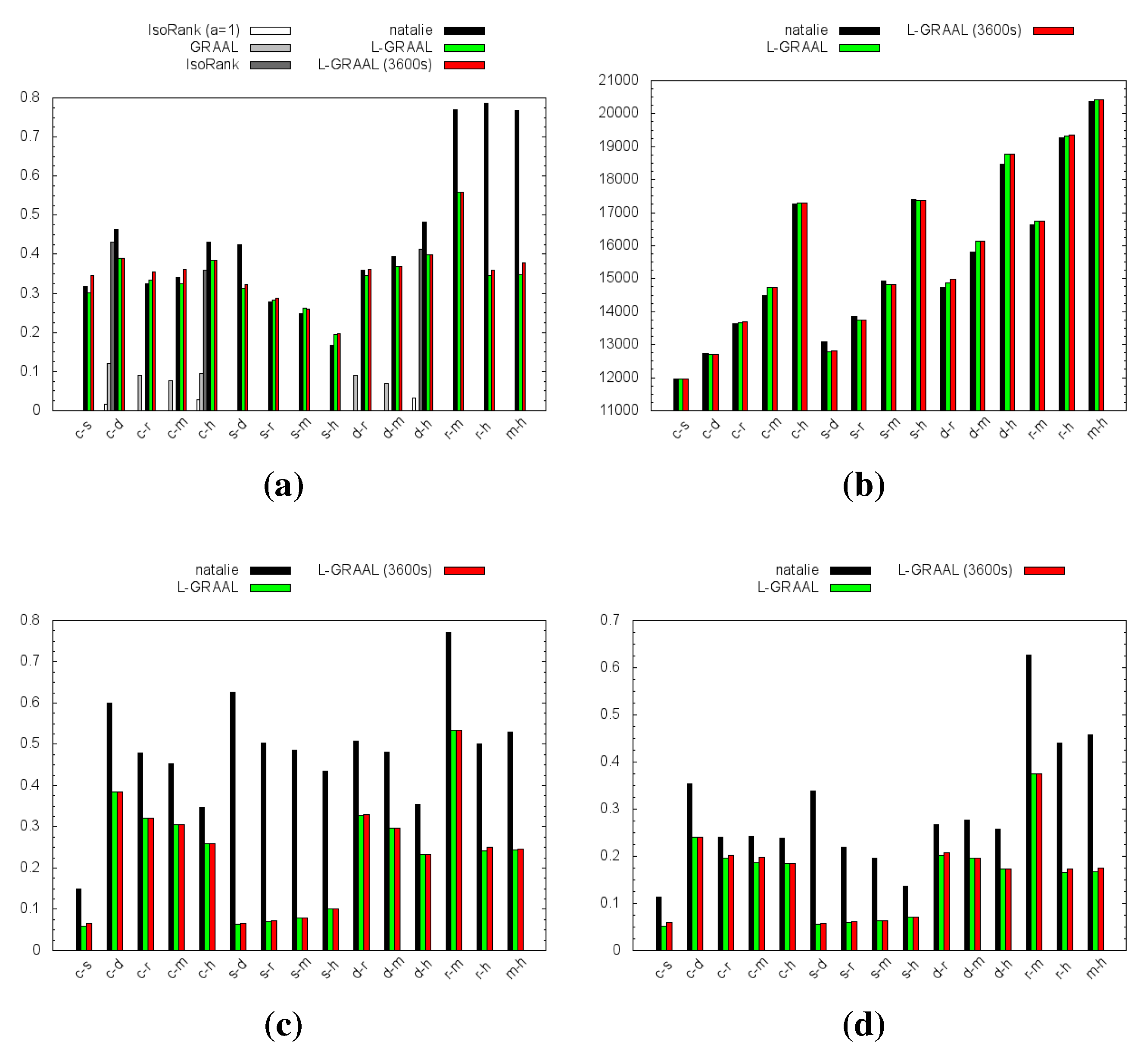
A popular evaluation metric for network alignments is edge correctness (EC), which is the number of conserved edges divided by the number of edges of the smaller network. This measure can be directly optimized, for example in Natalie 2.0, by setting the scoring function to $s\left(a\right)=\left|\right\{(v,w)\in E_1\mid (a\left(v\right),a\left(w\right))\in E_2\left\}\right|$. In addition, for Natalie 2.0 and L-GRAAL, we measured the size of the largest aligned connected component (LCC), and the recently proposed measures induced and symmetric substructure score (ICS and S3). ICS takes also matching non-edges into account and is defined as the number of matched edges divided by the number of edges in the subgraph of $G_2$ that is induced by the matching. The asymmetry in this measure is corrected for by the S3 measure, which is the fraction of matched edges between $G_1$ and the subnetwork of $G_2$ induced by the alignment. Note that it is easy to achieve perfect ICS or S3 values when alignments are defined as partial functions. In this case, matching, for example, two $K_3$ subgraphs of the input graphs would give a perfect score in terms of ICS or S3. For this reason, it is preferable to consult EC and LCC in addition.

As mentioned in Section 3, Natalie 2.0 as well as L-GRAAL can benefit greatly from using a sparse alignment graph. To that end, we use the e-values obtained from the all-against-all sequence alignment to prohibit biologically unlikely matchings by only considering protein-pairs whose e-value is at most 100. Note that this only applies to Natalie and L-GRAAL as both GRAAL and IsoRank consider the complete alignment graph. On each of the 15 instances, we ran GRAAL with three different random seeds and sampled the input parameter which balances the contribution of the graphlets with the node degrees uniformly within the allowed range of $[0,1]$. As for IsoRank, when setting the parameter α, which controls to what extent topological similarity plays a role, to the desired value of one, very poor results were obtained. Therefore we also sampled this parameter within its allowed range and re-evaluated the resulting alignments in terms of edge-correctness. Natalie was run with a time limit of 10 minutes CPU time and the standard settings $K=3$, $L=100$, $M=10$, $N=20$. L-GRAAL was run with a CPU time limit of 10 min as well as one hour. For both GRAAL and IsoRank, only the highest-scoring results were considered.

Figure 2. Performance of the four different methods for all-against-all species comparisons (15 alignment instances). Missing bars correspond to exceeded time/memory limits or software crashes. For LCC, ICS and S3 only Natalie 2.0 and L-GRAAL were compared. (a) Edge correctness (EC); (b) Size of largest connected component (LCC); (c) Induced Substructure Score (ICS); (d) Symmetric Substructure Score (S3).

Figure 2. Performance of the four different methods for all-against-all species comparisons (15 alignment instances). Missing bars correspond to exceeded time/memory limits or software crashes. For LCC, ICS and S3 only Natalie 2.0 and L-GRAAL were compared. (a) Edge correctness (EC); (b) Size of largest connected component (LCC); (c) Induced Substructure Score (ICS); (d) Symmetric Substructure Score (S3).

Figure 2 shows the results. IsoRank was only able to compute alignments for three out of the 15 instances. On the other instances IsoRank crashed, which may be due to the large size of the input networks. For GRAAL no alignments concerning sce could be computed, which is due to the large number of edges in the network: in 12 h only for 3% of the nodes the graphlet degree vector was computed. As for the last three instances, GRAAL crashed due to exceeding the memory limit inherent to 32-bit processes. Unfortunately no 64-bit executable was available. On the instances for which GRAAL could compute alignments, the alignment quality is poor when compared to the other methods. Natalie 2.0 outperforms the other methods in terms of edge correctness and outperforms L-GRAAL in terms of ICS and S3. The LCC values of both methods are similar.

4.2. GO Similarity

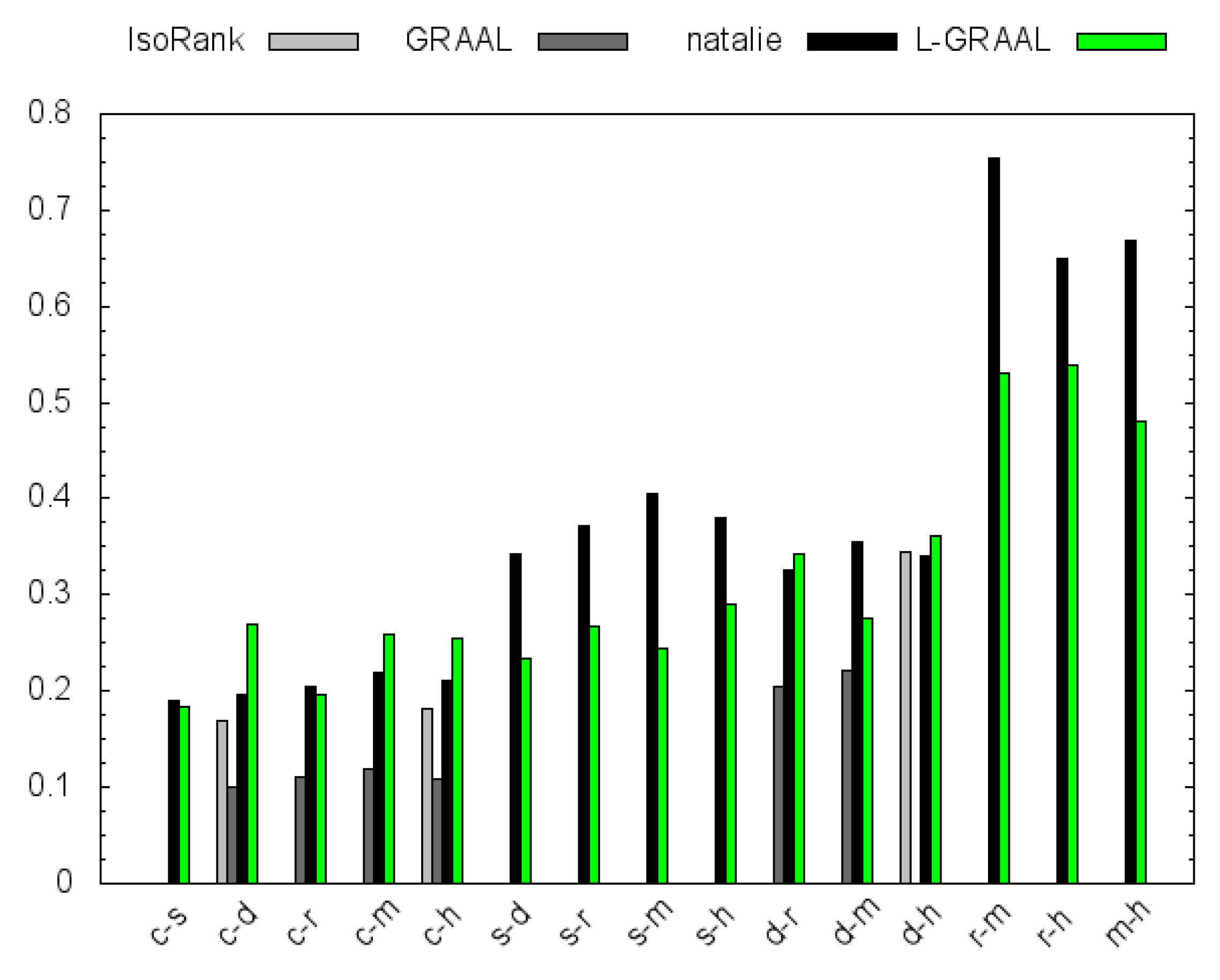
In order to measure the biological relevance of the obtained network alignments, we make use of the Gene Ontology (GO) [31]. For every node in each of the six networks, we obtained a set of GO annotations (see Table 1 for the exact numbers). Each annotation set was extended to a multiset by including all ancestral GO terms for every annotation in the original set. Subsequently, we employed a similarity measure that compares a pair of aligned nodes based on their GO annotations and also takes into account the relative frequency of each annotation [32]. Since the similarity measure assigns a score between 0 and 1 to every aligned node pair, the highest similarity score one can get for any alignment is the minimum number of annotated nodes in either of the networks. We therefore normalize the similarity scores by this quantity. Unlike the previous experiment, this time we considered the bitscores of the pairwise global sequence alignments. Similarly to the IsoRank and L-GRAAL parameter α, we introduced a parameter $\beta \in [0,1]$ such that the sequence part of the score has weight $(1-\beta )$ and the topology part has weight β. We sampled the weight parameters uniformly in the range $[0,1]$ for all methods. Figure 3 shows that on the smaller networks Natalie, L-GRAAL and IsoRank identify functionally coherent alignments with similar GO scores. However, Natalie outfperforms the other methods on many of the larger networks.

Figure 3. Biological relevance of the alignments measured via GO similarity.

Figure 3. Biological relevance of the alignments measured via GO similarity.

5. Conclusions

Inspired by results for the closely related quadratic assignment problem (QAP), we have presented new algorithmic ideas in order to make a Lagrangian relaxation approach for global network alignment practically useful and competitive. In particular, we have generalized a dual descent method for the QAP. We have found that combining this scheme with the traditional subgradient optimization method leads to fastest progress of upper and lower bounds.

Our implementation of the new method, Natalie 2.0, works well and fast when aligning biological networks, which we have shown in an extensive study on the alignment of cross-species PPI networks. We have compared Natalie 2.0 to the established and new state-of-the-art methods IsoRank, GRAAL and L-GRAAL, which aim at optimizing similar scoring functions. Our experiments show that the Lagrangian relaxation approach is a powerful method, which often outperforms the competitors in terms of quality of the results and running time.

Currently, all methods, including Natalie 2.0, approach the global network alignment problem heuristically, that is, the computed alignments are not guaranteed to be optimal solutions of the problem. While some approaches are intrinsically heuristic—both IsoRank and GRAAL, for instance, approximate the neighborhood of a node and then match it with a similar node—the inexactness in Natalie 2.0 and also L-GRAAL has two causes that we plan to address in future work: on the one hand, there may still be a gap between upper and lower bound of the Lagrangian relaxation approach after the last iteration. One could use these bounds in a branch-and-bound approach that will compute provably optimal solutions. On the other hand, we currently do not consider the complete bipartite alignment graph and may therefore miss optimal alignments. Here, preprocessing strategies, in the spirit of [33], which safely sparsify the input bipartite graph without violating optimality conditions, may be useful.

The independence of local problems (L${\text{D}}_{\lambda }^{ik}$) allows for straightforward parallelization, which would lead to an even faster method. Another improvement in running times might be achieved when considering more involved heuristics for computing the lower bound, such as local search. More functionally-coherent alignments can be obtained when considering a scoring function where node-to-node correspondences are not only scored via sequence similarity but also for instance via GO similarity. In certain cases, even negative weights for topological interactions might be desired in which case one needs to reconsider the assumption of entries of matrix W being positive.

References

1. Szklarczyk, D.; Franceschini, A.; Wyder, S.; Forslund, K.; Heller, D.; Huerta-Cepas, J.; Simonovic, M.; Roth, A.; Santos, A.; Tsafou, K.P.; et al. STRING v10: Protein-protein interaction networks, integrated over the tree of life. Nucleic Acids Res. 2015, 43. [Google Scholar] [CrossRef] [PubMed]
2. Sharan, R.; Ideker, T. Modeling cellular machinery through biological network comparison. Nat. Biotechnol. 2006, 24, 427–433. [Google Scholar] [CrossRef] [PubMed]
3. Kanehisa, M.; Goto, S.; Hattori, M.; Aoki-Kinoshita, K.F.; Itoh, M.; Kawashima, S.; Katayama, T.; Araki, M.; Hirakawa, M. From genomics to chemical genomics: New developments in KEGG. Nucleic Acids Res. 2006, 34. [Google Scholar] [CrossRef] [PubMed]
4. Alon, U. Network motifs: Theory and experimental approaches. Nat. Rev. Genet. 2007, 8, 450–461. [Google Scholar] [CrossRef] [PubMed]
5. Elmsallati, A.; Clark, C.; Kalita, J. Global alignment of protein-protein interaction networks: A survey. IEEE/ACM Trans. Comput. Biol. Bioinf. 2015, 99. [Google Scholar] [CrossRef] [PubMed]
6. Singh, R.; Xu, J.; Berger, B. Global alignment of multiple protein interaction networks with application to functional orthology detection. Proc. Natl. Acad. Sci. USA 2008, 105, 12763–12768. [Google Scholar] [CrossRef] [PubMed]
7. Klau, G.W. A new graph-based method for pairwise global network alignment. BMC Bioinf. 2009, 10. [Google Scholar] [CrossRef] [PubMed]
8. Kuchaiev, O.; Milenkovic, T.; Memisevic, V.; Hayes, W.; Przulj, N. Topological network alignment uncovers biological function and phylogeny. J. R. Soc. Interface 2010, 7, 1341–54. [Google Scholar] [CrossRef] [PubMed]
9. Patro, R.; Kingsford, C. Global network alignment using multiscale spectral signatures. Bioinformatics 2012, 28, 3105–3114. [Google Scholar] [CrossRef] [PubMed]
10. Neyshabur, B.; Khadem, A.; Hashemifar, S.; Arab, S.S. NETAL: A new graph-based method for global alignment of protein-protein interaction networks. Bioinformatics 2013, 29, 1654–1662. [Google Scholar] [CrossRef] [PubMed]
11. Aladağ, A.E.; Erten, C. SPINAL: Scalable protein interaction network alignment. Bioinformatics 2013, 29, 917–924. [Google Scholar] [CrossRef] [PubMed]
12. Chindelevitch, L.; Ma, C.Y.; Liao, C.S.; Berger, B. Optimizing a global alignment of protein interaction networks. Bioinformatics 2013, 29, 2765–2773. [Google Scholar] [CrossRef] [PubMed]
13. Hashemifar, S.; Xu, J. HubAlign: An accurate and efficient method for global alignment of protein-protein interaction networks. Bioinformatics 2014, 30, i438–i444. [Google Scholar] [CrossRef] [PubMed]
14. Vijayan, V.; Saraph, V.; Milenković, T. MAGNA++: Maximizing accuracy in global network alignment via both node and edge conservation. Bioinformatics 2015, 31. [Google Scholar] [CrossRef] [PubMed]
15. Clark, C.; Kalita, J. A multiobjective memetic algorithm for PPI network alignment. Bioinformatics 2015, 31, 1988–1998. [Google Scholar] [CrossRef] [PubMed]
16. Malod-Dognin, N.; Przulj, N. L-GRAAL: Lagrangian graphlet-based network aligner. Bioinformatics 2015, 31, 2182–2189. [Google Scholar] [CrossRef] [PubMed]
17. Natalie 2.0. Available online: http://software.cwi.nl/natalie (accessed on 15 November 2015).
18. El-Kebir, M.; Brandt, B.W.; Heringa, J.; Klau, G.W. NatalieQ: A web server for protein-protein interaction network querying. BMC Syst. Biol. 2014, 8. [Google Scholar] [CrossRef] [PubMed]
19. NatalieQ. Available online: http://www.ibi.vu.nl/programs/natalieq/ (accessed on 15 November 2015).
20. Karp, R.M. Reducibility Among Combinatorial Problems. In Complexity of Computer Computations; Miller, R.E., Thatcher, J.W., Eds.; Plenum Press: New York, NY, USA, 1972; pp. 85–103. [Google Scholar]
21. Lawler, E.L. The quadratic assignment problem. Manage Sci. 1963, 9, 586–599. [Google Scholar] [CrossRef]
22. Adams, W.P.; Johnson, T. Improved linear programming-based lower bounds for the quadratic assignment problem. DIMACS Ser. Discr. Math. Theor. Comput. Sci. 1994, 16, 43–77. [Google Scholar]
23. Kuhn, H.W. The Hungarian method for the assignment problem. Naval Res. Logist. Q. 1955, 2, 83–97. [Google Scholar] [CrossRef]
24. Munkres, J. Algorithms for the assignment and transportation problems. SIAM J. Appl. Math. 1957, 5, 32–38. [Google Scholar] [CrossRef]
25. Edmonds, J.; Karp, R.M. Theoretical improvements in algorithmic efficiency for network flow problems. J. ACM 1972, 19, 248–264. [Google Scholar] [CrossRef]
26. Edmonds, J. Path, trees, and flowers. Can. J Math 1965, 17, 449–467. [Google Scholar] [CrossRef]
27. Guignard, M. Lagrangean relaxation. Top 2003, 11, 151–200. [Google Scholar] [CrossRef]
28. Held, M.; Karp, R.M. The traveling-salesman problem and minimum spanning trees: Part II. Math. Progr. 1971, 1, 6–25. [Google Scholar] [CrossRef]
29. Caprara, A.; Fischetti, M.; Toth, P. A heuristic method for the set cover problem. Oper. Res. 1999, 47, 730–743. [Google Scholar] [CrossRef]
30. Egerváry Research Group on Combinatorial Optimization. LEMON Graph Library. Available online: http://lemon.cs.elte.hu/ (accessed on 15 November 2015).
31. Ashburner, M.; Ball, C.A.; Blake, J.A.; Botstein, D.; Butler1, H.; Cherry, J. M.; Davis, A.P.; Dolinski, K.; Dwight, S.S.; Eppig, J.T.; et al. Gene Ontology: Tool for the unification of biology. Nat. Genet. 2000, 25, 25–29. [Google Scholar] [CrossRef] [PubMed]
32. Couto, F.M.; Silva, M.J.; Coutinho, P.M. Measuring Semantic Similarity between Gene Ontology Terms. Data Knowl. Eng. 2007, 61, 137–152. [Google Scholar] [CrossRef]
33. Wohlers, I.; Andonov, R.; Klau, G.W. Algorithm Engineering for optimal alignment of protein structure distance matrices. Optim. Lett. 2011, 5, 421–433. [Google Scholar] [CrossRef] [Green Version]