Semi-Supervised Classification Based on Mixture Graph

Abstract

Graph-based semi-supervised classification heavily depends on a well-structured graph. In this paper, we investigate a mixture graph and propose a method called semi-supervised classification based on mixture graph (SSCMG). SSCMG first constructs multiple k nearest neighborhood (kNN) graphs in different random subspaces of the samples. Then, it combines these graphs into a mixture graph and incorporates this graph into a graph-based semi-supervised classifier. SSCMG can preserve the local structure of samples in subspaces and is less affected by noisy and redundant features. Empirical study on facial images classification shows that SSCMG not only has better recognition performance, but also is more robust to input parameters than other related methods.

1. Introduction

Many real-world pattern classification and data mining applications are often confronted with a typical problem that is lacking of sufficient labeled data, since labeling samples usually requires domain-specific experts [1,2]. Supervised classifiers, trained only on such scarcely labeled samples, often can not have a good generalization ability. With the development of high-throughput techniques, a large number of unlabeled data can be easily accumulated. If we take these labeled samples as unlabeled ones and train unsupervised learners (i.e., clustering) on all the unlabeled samples, the valuable information in labeled samples is wasted. That is because the label information should be regarded as prior information, which can be used to boost the performance of a classifier [3]. Therefore, it is important to develop techniques that leverage both labeled and unlabeled samples.

Semi-supervised learning aims to leverage labeled and unlabeled samples to achieve a learner with good generalization ability [1]. In this paper, we focus on semi-supervised classification, and more specifically on graph-based semi-supervised classification (GSSC). In GSSC, labeled and unlabeled samples are taken as nodes (or vertices) of a weighted graph, and the edge weights reflect the similarity between samples [1]. Various effective GSSC methods have been proposed in the last decade. To name a few, Zhu et al. [4] utilized Gaussian fields and harmonic functions (GFHF) on a k nearest neighborhood (kNN) graph to predict the labels of unlabeled samples via label propagation on the graph. Zhou et al. [5] studied a learning with local and global consistence (LGC) approach on a completely connected graph based on the consistency assumption. These two methods can be regarded as label propagation on a graph under different assumptions or schemes [1]. Most GSSC methods focus on how to leverage labeled and unlabeled samples but pay little attention to construct a well-structure graph that faithfully reflects the distribution of samples. For low dimensional samples, these GSSC methods can achieve good performance by using a simple kNN graph. When dealing with high dimensional instances, their performance often drops sharply, since the noisy and redundant features of high dimensional samples destroy the underlying distance (or similarity) between samples [3,6].

Recently, researchers recognized the importance of graph in GSSC and proposed various graph optimization based semi-supervised classification methods [1,7,8,9,10]. Zhu [1] gave a comprehensive literature review on semi-supervised learning. Here, we just name a few most related and representative methods, which will be used for experimental comparison. Wang et al. [11] used an $l_2$ graph [12], optimized by minimizing the $l_2$-norm regularized reconstruction error of locally linear embedding [13], and studied a linear neighborhood propagation (LNP) approach. Liu et al. [7] took advantage of iterative nonparametric matrix learning to construct a symmetric adjacent graph and proposed a robust multi-class graph transductive (RMGT) classification method. In addition, Fan et al. [9] constructed an $l_1$ graph by the coefficients of $l_1$-norm regularized sparse representation [14] to perform semi-supervised classification. Zhao et al. [10] suggested a compact graph based semi-supervised learning (CGSSL) method for image annotation. This method constructs a compact $l_2$ graph by utilizing not only the neighborhood samples of a sample, but also the neighborhood samples of its reciprocal neighbors. However, the effectiveness of these methods is not as good as expected when dealing with high dimensional data, since high dimensional data have a lot of noisy and redundant features, and it is difficult to optimize a graph distorted by these noisy features [2,15].

More recently, some researchers studied how to synthesize multiple graphs, derived from multiple data sources or multiple modules data, for semi-supervised classification [16]. Wang et al. [17], Karasuyama and Mamitsuka [18], Shiga and Mamitsuka [19] and Yu et al. [20] explored different techniques (i.e., multiple kernel learning [21], kernel target alignment [22]) to assign different weights to the graphs and then weighted combined these graphs into a composite graph for semi-supervised classification. A number of researchers have applied the random subspace method (RSM) [23] to semi-supervised classification [2,15] and dimensionality reduction [24]. Particularly, Yu et al. [2] proposed a GSSC method called semi-supervised ensemble classification in subspaces (SSEC in short). SSEC firstly constructs several kNN graphs in the random subspaces of samples; then, it trains several semi-supervised linear classifiers on these graphs, one classifier for each graph; next, it combines these classifiers into an ensemble classifier for prediction. The empirical study shows that the base classifiers trained on these simple kNN graphs outperform the classifier trained in the original space, and the ensemble classifier also works better than other graph optimization based semi-supervised classifiers (i.e., LNP and RMGT) and some representative ensemble classifiers (i.e., Random Forest [25] and Rotation Forest [26]).

In this paper, motivated by these observations, we investigate a mixture graph combined by multiple kNN graphs constructed in the subspaces, and study a semi-supervised classification method on this mixture graph ((semi-supervised classification based on mixture graph SSCMG)). Particularly, SSCMG first constructs multiple kNN graphs in different random subspaces (like the random subspace scheme in [23]) of samples, and then combines these graphs into a mixture graph. Finally, SSCMG incorporates this mixture graph into GFHF [4], a representative GSSC method, for semi-supervised classification. Since the distance metric is more reliable in the subspace than that in the original space and the mixture graph is constructed in subspaces, the mixture graph is less suffered from the noisy samples and features. Besides, it is able to hold complicated geometric distribution as the diversity of random subspaces. Experimental comparison with other related methods shows that SSCMG not only has higher classification accuracy, but also has wide ranges of effective input parameters. The main difference between SSCMG and aforementioned GFHF, LGC, LNP, RMGT and CGSSL is that SSCMG uses a mixture graph combined by multiple kNN graphs constructed in the subspaces, whereas the other methods just utilize (or optimize) a single graph alone. SSEC trains several semi-supervised linear classifiers based on kNN graphs constructed in randomly partitioned subspaces and incorporates these classifiers into an ensemble classifier for prediction. In contrast, SSCMG integrates multiple kNN graphs constructed in random subspaces into a mixture graph, and then trains one semi-supervised classifier based on the mixture graph.

In summary, the main contributions of this paper are summarized as follows: (1) A semi-supervised classification based on mixture graph (SSCMG) method is proposed for high-dimensional data classification; (2) Extensive experimental study and analysis demonstrate that SSCMG achieves higher accuracy and it can be more robust to input parameters than other related methods; (3) Mixture graph works better than the graph optimized by a single kNN graph alone, and it can be used as a good alternative graph for GSSC methods on high dimensional data.

The rest of this paper is structured as follows: Section 2 describes the procedure of GFHF and introduces the construction of mixture graph. In Section 3, extensive experiments are conducted to study the performance and parameter sensitivity of SSCMG. Conclusions and future work are provided in Section 4.

2. Methodology

In this section, we introduce GFHF first and then provide the procedures of the mixture graph.

2.1. Gaussian Fields and Harmonic Functions

Suppose there are $n=l+u$ samples ${\mathbf{x}}_i\in {\mathbb{R}}^D$ ($1\le i\le n$), organized in a matrix $\mathbf{X}=[{\mathbf{x}}_1;{\mathbf{x}}_2;\cdots ;{\mathbf{x}}_l;{\mathbf{x}}_{l+1};\cdots ;{\mathbf{x}}_{l+u}]$, where l is the number of labeled samples, u is the number of unlabeled samples. ${\mathbf{y}}_i\in {\mathbb{R}}^C$ is the label vector of the i-th samples, if ${\mathbf{x}}_i$ belongs to the c-th class then $y_{ic}=1$; otherwise $y_{ic}=0$. Obviously, ${\mathbf{y}}_i=\mathbf{0}$ means the label of ${\mathbf{x}}_i$ is unknown (or unlabeled). The target is to predict the labels of u unlabeled samples.

Various semi-supervised classifiers can be used to infer the labels of these u unlabeled samples [1]. In this paper, we choose GFHF [4] for its simplicity and wide-application. To be self-consistent and to discuss the importance of graph for GSSC methods, the main procedures of GFHF are listed below and more details of GFHF can be found in reference [4].

(1). Construct a weighted kNN graph G and let $\mathbf{W}={\left[w_{ij}\right]}_{n\times n}$ be the association matrix of G. $w_{ij}$ is specified as follows:

$$w_{ij}=\left\{\begin{array}{c}{e}^{-\frac{{∥{\mathbf{x}}_i-{\mathbf{x}}_j∥}_2^2}{{\sigma }^2}},\mathrm{if}{\mathbf{x}}_j\in {\mathcal{N}}_k\left({\mathbf{x}}_i\right)\mathrm{or}{\mathbf{x}}_i\in {\mathcal{N}}_k\left({\mathbf{x}}_j\right)\hfill \\ 0,\mathrm{otherwise}\hfill \end{array}\right.$$

(1)

where σ is a scalar parameter to control the decaying rate of distance between ${\mathbf{x}}_i$ and ${\mathbf{x}}_j$, and it is called Gaussian kernel width. ${\mathcal{N}}_k\left({\mathbf{x}}_i\right)$ includes k nearest neighborhood samples of ${\mathbf{x}}_i$. $w_{ij}$ ensures two nearby samples have a large similarity and two faraway samples have a small or zero similarity.

(2). GFHF assumes nearby samples having similar labels and propagates the labels of labeled samples in G to infer the labels of unlabeled samples in G. Particularly, it optimizes the predictive function $f\left(\mathbf{x}\right)\in {\mathbb{R}}^C$ on n samples as follows:

$$\underset{f}{min}(\infty \sum _{i=1}^l\left(\right||{\mathbf{y}}_i-f\left({\mathbf{x}}_i\right){\left|\right|}_2^2)+\frac{1}{2}\sum _{i,j=1}^n{w}_{ij}\left|\right|f\left({\mathbf{x}}_i\right)-f\left({\mathbf{x}}_j\right){\left|\right|}_2^2)$$

(2)

where $f\left({\mathbf{x}}_i\right)\in {\mathbb{R}}^C$ is the predicted likelihood of ${\mathbf{x}}_i$ with respect to C classes. To ensure the prediction on the first l samples be the same with their initial labels, an ∞ weight is assigned to the first term. The second term is to ensure nearby samples having similar predicted likelihoods. Equation (2) can be rewritten as:

$$\underset{f}{min}(\infty \sum _{i=1}^l\left(\right||{\mathbf{y}}_i-f\left({\mathbf{x}}_i\right){\left|\right|}_2^2)+{\mathbf{f}}^T\mathbf{L}\mathbf{f})$$

(3)

where $\mathbf{f}=[f\left({\mathbf{x}}_1\right);f\left({\mathbf{x}}_2\right);\cdots ;f\left({\mathbf{x}}_n\right)]$, $\mathbf{L}=\mathbf{D}-\mathbf{W}$ is the graph Laplacian matrix [27], $\mathbf{D}$ is a diagonal matrix with ${\mathbf{D}}_{ii}={\sum }_j{\mathbf{W}}_{ij}$.

(3). To get the harmonic solution of Equation (3), $\mathbf{W}$ is divided into four blocks as follows:

$$\mathbf{W}=\left[\begin{array}{cc}{\mathbf{W}}_{ll}& {\mathbf{W}}_{lu}\\ {\mathbf{W}}_{ul}& {\mathbf{W}}_{uu}\end{array}\right]$$

(4)

where ${\mathbf{W}}_{ll}\in {\mathbb{R}}^{l\times l}$ describes the pairwise similarity between the first l samples, ${\mathbf{W}}_{lu}\in {\mathbb{R}}^{l\times u}$ (or ${\mathbf{W}}_{ul}$) represents the similarity between the first l labeled samples and u unlabeled samples, and ${\mathbf{W}}_{uu}\in {\mathbb{R}}^{u\times u}$ captures the similarity between u unlabeled samples. Suppose ${\mathbf{f}}_u\in {\mathbb{R}}^{u\times C}$ be the predicted likelihoods on u unlabeled samples and ${\mathbf{f}}_l\in {\mathbb{R}}^{l\times C}$ be the predictions on the first l labeled samples. The explicit solution of Equation (3) is:

$${\mathbf{f}}_u={({\mathbf{D}}_{uu}-{\mathbf{W}}_{uu})}^{-1}{\mathbf{W}}_{ul}{\mathbf{f}}_l$$

(5)

From Equation (5), it is easy to observe that $\mathbf{W}$ is the deciding factor of ${\mathbf{f}}_u$, or in other words the graph constructed in Equation (1) determines the label of unlabeled samples.

Most GSSC methods can obtain good results on low dimensional data. However, when dealing with high-dimensional data, the effectiveness of these classifiers is often significantly reduced [2]. The reason is that there are many noisy and redundant features in high-dimensional data and these features distort the neighborhood relationship (or similarity) between samples [3,6,15]. Given that, the graph-based classifiers can not correctly and effectively use the labels associated with a sample’s neighbors to predict its label. In fact, some researchers already claimed that graph determines the performance of graph-based semi-supervised learning [1,7] and graph-based dimensionality reduction [28]. Maier et al. [29] found that a graph-based clustering approach has two optimal clustering solutions on two different graphs from the same dataset.

2.2. Mixture Graph Construction

Yu et al. [2] observed that a semi-supervised linear classifier based on a kNN graph in the subspace can achieve higher accuracy than the classifier based on a kNN graph in the original space. This observation indicates that a kNN graph in the high dimensional space is often suffered from noisy and redundant features. In contrast, a kNN graph in the low dimensional space is less suffered from the redundant and noisy features. In addition, Yu et al. [15] found that an $l_1$ graph constructed in the subspace is also less suffered from noise features than the $l_1$ graph in the original space. Inspired by these observations, we investigate a mixture graph, combined by kNN graphs constructed in several random subspaces of original space, for semi-supervised classification. The detailed procedure of mixture graph is listed as follows:

(1). Randomly sampling d feature indices without replacement, and project $\mathbf{X}$ into ${\mathbf{X}}^t=[{\mathbf{x}}_1^t;{\mathbf{x}}_2^t;\cdots ;{\mathbf{x}}_n^t]\in {\mathbb{R}}^{n\times d}$, ${\mathbf{x}}_i^t$ is consisted of the sampled d features of ${\mathbf{x}}_i$.

(2). Construct a kNN graph on ${\mathbf{X}}^t$, and define the corresponding association matrix as:

$${\mathbf{W}}_{ij}^t=\left\{\begin{array}{c}1,\mathrm{if}{\mathbf{x}}_j^t\in {\mathcal{N}}_k\left({\mathbf{x}}_i^t\right)\mathrm{or}{\mathbf{x}}_i^t\in {\mathcal{N}}_k({\mathbf{x}}_j^t)\hfill \\ 0,\mathrm{otherwise}\hfill \end{array}\right.$$

(6)

where ${\mathcal{N}}_k\left({\mathbf{x}}_i^t\right)$ includes k nearest neighborhood samples of ${\mathbf{x}}_i^t$, and the neighborhood relationship is determined by the Euclidean distance between samples. In this way, we can construct a kNN graph $G^t$ and define its association matrix ${\mathbf{W}}^t$ in the t-th subspace.

(3). Repeat the above two steps T times and thus T graphs can be constructed in T random subspaces, one graph for each subspace. Then, these kNN graphs can be integrated into a mixture graph and its association matrix is defined as follows:

$${\mathbf{W}}_{ij}^{mg}=\frac{1}{T}\sum _{t=1}^T{\mathbf{W}}_{ij}^t$$

(7)

Since the mixture graph is combined with T graphs constructed in random subspaces, the impact of noisy and redundant features is reduced. The mixture graph can not only hold more complicated geometric distribution of samples than any of the T graphs as the diversity of random subspaces, but also be less sensitive to k than a single kNN graph. From the viewpoint of ensemble learning [30] that the accuracy of an ensemble classifier is no smaller than the average accuracy of base classifiers; thus, the mixture graph avoids the risk of choosing a bad kNN graph. Some recent methods (i.e., diffuse interfaces [31], p-Laplacian [32]) were proposed to identify relevant features and to discard noisy features for semi-supervised learning. These methods are reported to perform well on samples with a large number of noisy features. In this case, our mixture graph may not work well as supposed. However, p-Laplacian can be borrowed by the mixture graph to discard these noisy features.

To investigate these potential advantages of mixture graph, we substitute $\mathbf{W}$ in Equation (1) with mixture graph ${\mathbf{W}}^{mg}$ and then perform semi-supervised classification on ${\mathbf{W}}^{mg}$ to predict the labels of unlabeled samples. In this way, we propose a method called Semi-Supervised Classification based on Mixture Graph (SSCMG). We study the characteristics of mixture graph by comparing it with several representative GSSC methods (i.e., RMGT [7], LNP [11], CGSSL[10]) and analyze its sensitivity under different values of input parameter.

3. Experiment

In this section, we conduct experiments on four publicly available face datasets to study the effectiveness of SSCMG. The face datasets used in the experiments are ORL [33], CMU PIE [34], AR [35], and extended YaleB [36]. ORL consists of 40 individuals with 10 images per person. We aligned and resized ORL images into 64 × 64 pixels in grey scale, thus each image can be viewed as a point in the 4096-dimensional space. CMU PIE face dataset contains 41,368 face images from 68 individuals. The face images were captured under varying pose, illumination and expression conditions, and we chose a subset (Pose27) of CMU PIE as the second dataset. Pose27 includes 3329 face images from 68 individuals. Before the experiments, we resized the images to 64 × 64 pixels and each image is an 8 bit grayscale image. AR face dataset includes over 4000 color face images from 126 people (70 men and 56 women). In the experiments, 2600 images of 100 people (50 men and 50 women) were used. We aligned and resized these images into 42 × 30 pixels and then normalized them into 8 bit grayscale, thus each image is a point in the 1260-dimensional space. YaleB consists of 21,888 single light source images of 38 individuals each captured under 576 viewing conditions (9 × 64 illumination conditions). We chose a subset that contains 2414 images and resized these images into 32 × 32 pixels, with 256 gray level per pixel, so each image is a 1024-dimensional vector. ORL and extended yaleB can be downloaded from the link in reference [37].

To comparatively study the performance of SSCMG, we take several representative methods as comparing methods, which include GFHF [4], LNP [11], RMGT [7], LGC [5], CGSSL [10]. We regard the classification accuracy on testing samples as the comparative index, and the higher the accuracy, the better the performance. Gaussian kernel used for graph construction can often be improved upon by using the ‘local scaling’ method [31,38]. We utilize local scaling to adjust the graph defined in Equation (1) and name GFHF on the adjusted graph as LGFHF. The diffuse interfaces model in [31] is proposed for binary classification and it is not so straightforward for multi-class datasets. Since the target of this study is to investigate the effectiveness of mixture graph for semi-supervised classification and the proposed SSCMG is a special case of p-Laplacian with $p=2$, we do not compare SSCMG with the diffuse interfaces model and p-Laplacian with different p values. In the following experiments, we firstly apply principal component analysis (PCA) [3] to project each facial image into a 100-dimensional vector, and then use different methods to predict the labels of unlabeled images. For convenience, notations used in the experiments are listed in Table 1.

Table 1. Notations used in the experiments.

Notation	Means
n	Number of labeled and unlabeled samples
l	Number of labeled samples
C	Number of classes
k	Neighborhood size
T	Number of subspaces
d	Dimensionality of random subspace
$Ls$	Number of labeled samples per class

Table 1. Notations used in the experiments.

Notation	Means
n	Number of labeled and unlabeled samples
l	Number of labeled samples
C	Number of classes
k	Neighborhood size
T	Number of subspaces
d	Dimensionality of random subspace
$Ls$	Number of labeled samples per class

In the experiments, if without extra specification, α in LGC [5] is set to 0.01, σ in Equation (1) is set to the average Euclidean distance between n samples, and k is fixed as 3 for all the methods that based on a kNN graph. T and d are set to 70 and 40, respectively. Other parameters of these comparing methods are kept the same as reported in the original papers. The sensitivity of these input parameters will be studied later. To reduce random effect, all reported results are the average of 20 independent runs. In each run, the training set and testing set are randomly partitioned.

3.1. Performance on Different Datasets

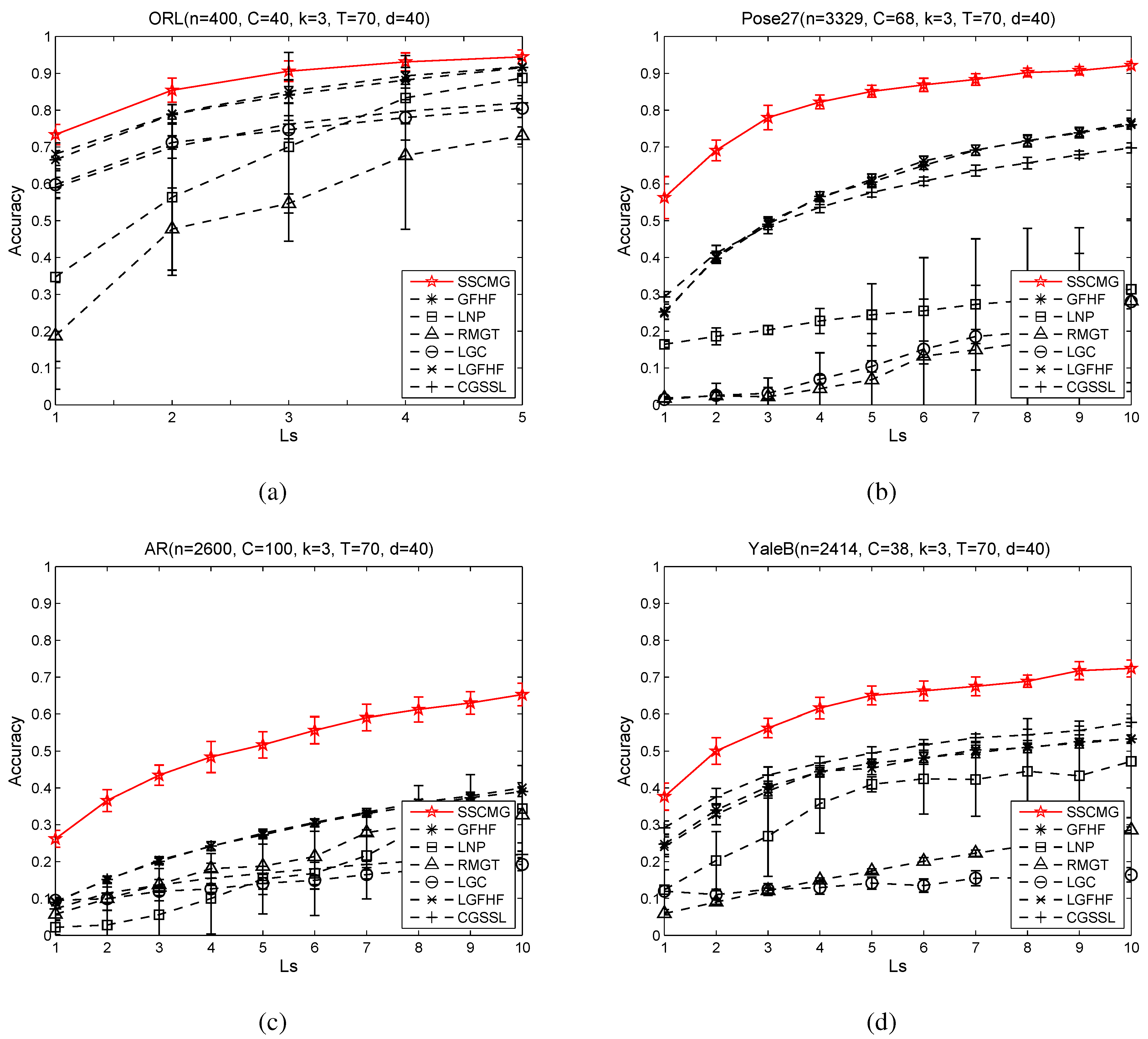
In order to study the performance of SSCMG under different number of labeled images per people, we conduct experiments on ORL with $Ls$ rising from 1 to 5, and on the other three datasets with $Ls$ increasing from 1 to 10. The corresponding results are revealed in Figure 1. Each class in the four datasets has an equal (or nearly equal) number of samples as other classes, so the classes are balanced. Each dataset has more than 30 classes and the accuracy per class cannot be visualized in Figure 1. Given these reasons, we report the average accuracy for all the classes on each dataset.

Figure 1. The performance of SSCMG on different $Ls$ values. (a) Accuracy vs. $Ls$ (ORL); (b) Accuracy vs. $Ls$ (Pose27); (c) Accuracy vs. $Ls$ (AR); (d) Accuracy vs. $Ls$ (YaleB).

Figure 1. The performance of SSCMG on different $Ls$ values. (a) Accuracy vs. $Ls$ (ORL); (b) Accuracy vs. $Ls$ (Pose27); (c) Accuracy vs. $Ls$ (AR); (d) Accuracy vs. $Ls$ (YaleB).

From these four sub-figures, it is easy to observe that SSCMG achieves better performance than these comparing methods on all facial datasets and GFHF almost ranks second among these comparing methods. Although SSCMG, LGFHF and GFHF are based on the same objective function, SSCMG always outperforms the latter two. That is because SSCMG utilizes a mixture graph combined by multiple kNN graphs defined in the subspaces, whereas the latter two depend on a single kNN graph constructed in the PCA reduced space. This observation not only justifies the statement that graph determines the performance of GSSC methods, but also supports our motivation to utilize mixture graph for semi-supervised classification. LGFHF is slightly superior to GFHF. This fact indicates local scaling technique can only improve the kNN graph in a small scale. LGC often loses to other methods. The reason is that LGC utilizes a fully connected graph rather than a kNN graph, and this fully connected graph is more heavily distorted by noisy features. RMGT and LNP apply different techniques to optimize a kNN graph, but their accuracies are almost always lower than that of SSCMG. The cause is that optimizing a kNN graph that distorted by noisy features is rather difficult. CGSSL uses a compact $l_2$ graph and it often outperforms LNP, which is based on a non-compact $l_2$ graph, but CGSSL is always outperformed by SSCMG. These facts suggest that optimizing an $l_2$ graph alone can only improve the performance in a small range, and it may not result in an optimal graph for semi-supervised classification.

As the number of labeled samples ($Ls$) increasing, the accuracy of SSCMG and other methods climbs steadily, for more labeled samples can often help to acquire a more accurate classifier. RMGT asks for a number of labeled samples to learn an optimized graph, but available labeled samples are not sufficient to optimize a good graph for RMGT. From these observations, we can conclude that mixture graphs can be used as a good alternative graph for GSSC methods on high dimensional data.

3.2. Sensitivity Analysis with Respect to Neighborhood Size

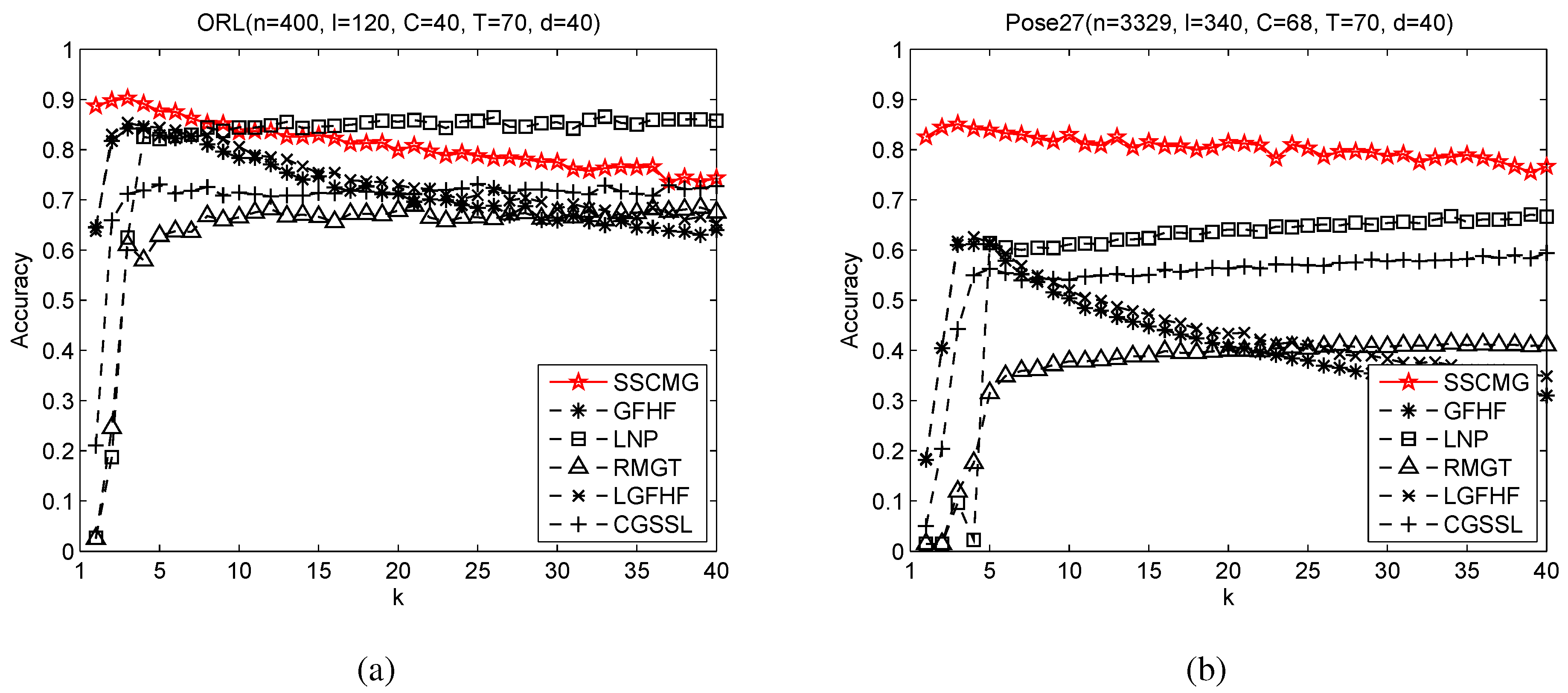
It is found that neighborhood size k of kNN graph can influence the results of GSSC. To investigate the sensitivity of SSCMG under different k values, we conduct experiments on ORL and Pose27. In the experiments, we fix $Ls$ as 3 on ORL and as 5 on Pose27, we then vary k from 1 to 40. We also include the results of other comparing methods that utilize a kNN graph and report the results in Figure 2.

Figure 2. Sensitivity under different values of k. (a) Accuracy vs. k (ORL); (b) Accuracy vs. k (Pose27).

Figure 2. Sensitivity under different values of k. (a) Accuracy vs. k (ORL); (b) Accuracy vs. k (Pose27).

From Figure 2, we can observe that SSCMG achieves better performance and it is less sensitive to k than other comparing methods when $k\le 10$. However, as k increasing, its accuracy downgrades gradually. This is because a large value of k means choosing more neighbors of a sample, so the constructed mixture graph is becoming denser and more noisy edges are included. On the other hand, the accuracy of GFHF and LGFHF first rise sharply as k increasing and then reduce gradually. The accuracy of LNP, RMGT and CGSSL increase as k rising and become relatively stable, and these methods sometimes get comparable (or better) results with SSCMG on ORL. The reason is that these three methods need a large number of neighbors to optimize a kNN graph for semi-supervised classification. CGSSL utilizes a compact $l_2$ graph by using the direct neighborhood samples of a sample and the neighborhood samples of its reciprocal neighbors. As k increasing, more neighborhood samples are included and thus the similarity between samples is more distorted by noisy neighbors. Given that, CGSSL loses to LNP, which is also based on an $l_2$ graph, but LNP only utilizes the direct neighborhood samples of a sample. As k increasing, the accuracy of GFHF and LGFHF on ORL and Pose27 downgrades much more than that of SSCMG, this observation suggests that mixture graph is less suffered from the choice of k than a single kNN graph. Figure 2 also shows that it is difficult to set a suitable k for GSSC methods. In contrast, there is a clear pattern and it is easy to select a suitable k for SSCMG. Although SSCMG, LGFHF and GFHF share the same classifier, the performance of SSCMG is always more stable than LGFHF and GFHF. This observation also justifies the advantage of mixture graph for GSSC.

3.3. Sensitivity Analysis with Respect to Dimensionality of Random Subspace

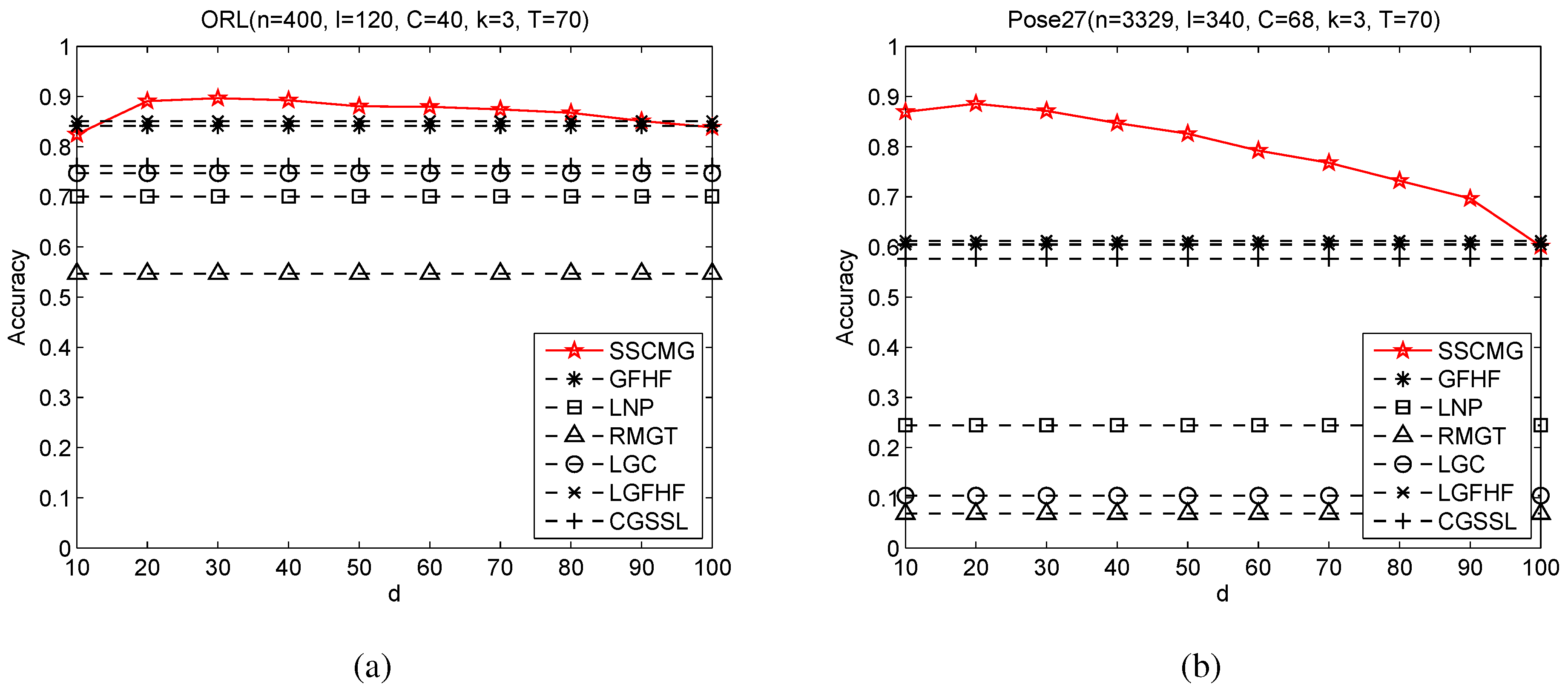
The dimensionality of random subspace is an influential parameter for the random subspace method [2,23]. To study the sensitivity of mixture graph with respect to the dimensionality of random subspace, we conduct two experiments on ORL and Pose27 with d varying from 10 to 100. The corresponding experimental results are reported in Figure 3. For reference, we also include the results of GFHF, LGFHF, LNP, RMGT, LGC and CGSSL in Figure 3.

Figure 3. Sensitivity under different values of d. (a) Accuracy vs. d (ORL); (b) Accuracy vs. d (Pose27).

Figure 3. Sensitivity under different values of d. (a) Accuracy vs. d (ORL); (b) Accuracy vs. d (Pose27).

From Figure 3, we can observe that the accuracy of SSCMG increases slightly as d rising at first and then turns to downgrade, especially on Pose27. The reason is twofold: (i) when d is very small (i.e., $d=10$), there are too few features to construct a graph that describes the distribution of samples projected in that subspace; (ii) as d is close to 100, more and more noisy features are included into the subspace and hence the graph is more and more distorted by noisy features. When $d=100$ all the features are included, these T graphs are the same, and thus the performance of SSCMG is similar to that of GFHF. Overall, irrespective of the setting of d, the performance of SSCMG is always no worse than that of GFHF. However, how to choose an effective value of d (or design a graph less suffered from d) is still a future pursue.

3.4. Sensitivity Analysis with Respect to Number of Random Subspaces

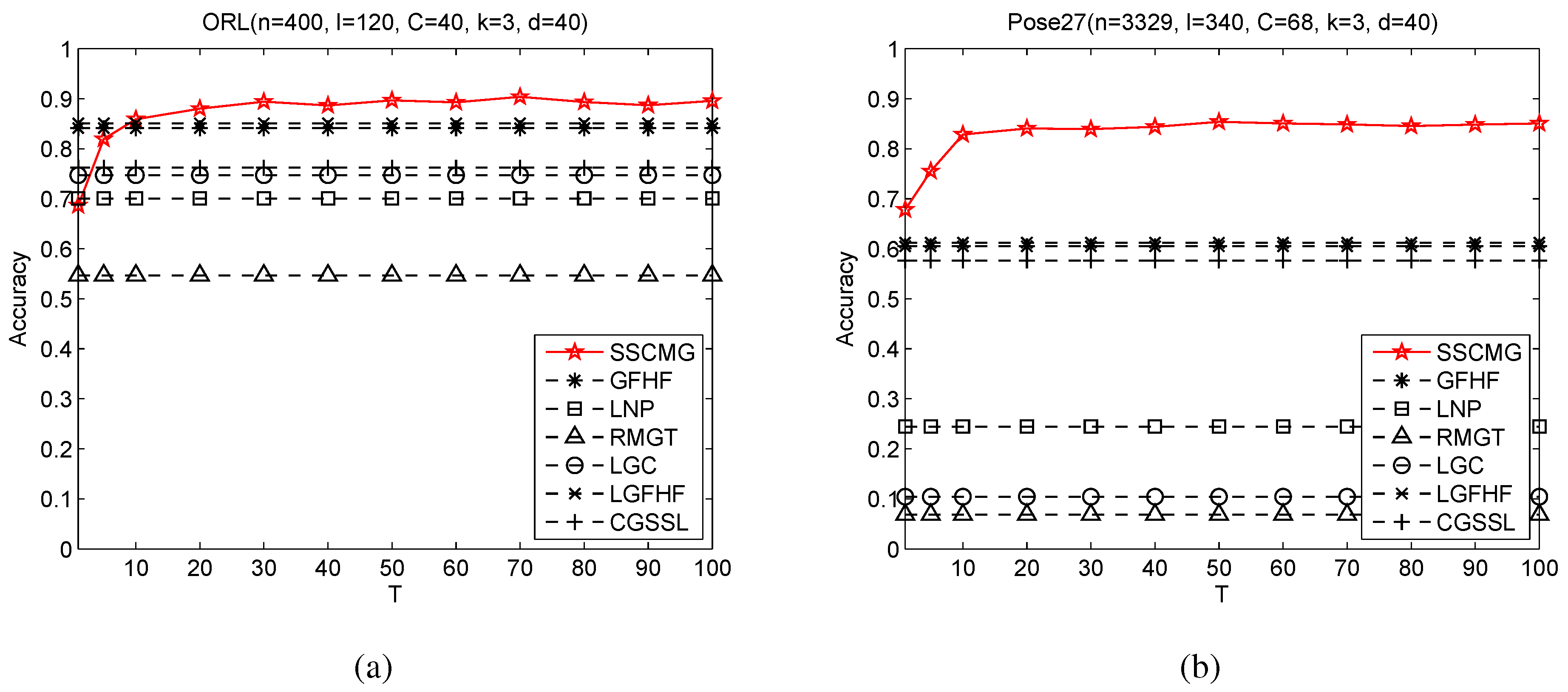
The number of random subspaces is another influential parameter of random subspace method. To explore the performance of SSCMG under different number of random subspaces, additional experiments are conducted on ORL and Pose27 with T rising from 1 to 100, and the corresponding results are shown in Figure 4.

Figure 4. Sensitivity under different values of T. (a) Accuracy vs. T (ORL); (b) Accuracy vs. T (Pose27).

Figure 4. Sensitivity under different values of T. (a) Accuracy vs. T (ORL); (b) Accuracy vs. T (Pose27).

From Figure 4, we can clearly observe that when $T<20$, the accuracy of SSCMG is relatively low, even lower than that of GFHF on ORL. The accuracy of SSCMG increases as T rising, and it reaches to relatively stable when $T\ge 20$. The cause is that too few kNN graphs in the subspaces can not capture the distribution of samples. Overall, these experimental results suggest that SSCMG can easily choose a suitable value of T in a wide range.

4. Conclusions and Future Work

In this paper, we studied a mixture graph, integrated by several kNN graphs constructed in the subspaces, and proposed a method called semi-supervised classification based on mixture graph (SSCMG). Experimental results on four publicly facial image datasets demonstrate that SSCMG not only achieves better results than other related methods, but also is less suffered from input parameters. In future work, we want to integrate graphs by setting different weights to these graphs and selectively integrate sub-graphs of each input graph for graph-based semi-supervised learning.