Article

Pulmonary Nodule Detection from X-ray CT Images Based on Region Shape Analysis and Appearance-based Clustering

1
Graduate School of Systems and Information Engineering, University of Tsukuba, 305-8573, Japan
2
Faculty of Engineering, Information and Systems, University of Tsukuba, 305-8573, Japan
*
Author to whom correspondence should be addressed.
Algorithms 2015, 8(2), 209-223; https://doi.org/10.3390/a8020209
Submission received: 24 December 2014 / Revised: 6 March 2015 / Accepted: 27 April 2015 / Published: 8 May 2015

Abstract

:
In this paper, we propose a detection method of pulmonary nodules in X-ray computed tomography (CT) scans by use of three image filters and appearance-based k-means clustering. First, voxel values are suppressed in radial directions so as to eliminate extra regions in the volumes of interest (VOIs). Globular regions are enhanced by moment-of-inertia tensors where the voxel values in the VOIs are regarded as mass. Excessively enhanced voxels are reduced based on displacement between the VOI centers and the gravity points of the voxel values in the VOIs. Initial nodule candidates are determined by these filtering processings. False positives are reduced by, first, normalizing the directions of intensity distributions in the VOIs by rotating the VOIs based on the eigenvectors of the moment-of-inertia tensors, and then applying an appearance-based two-step k-means clustering technique to the rotated VOIs. The proposed method is applied to actual CT scans and experimental results are shown.

1. Introduction

Lung cancer is the most common cause of death among all cancers worldwide. To cope with this serious situation, mass screening for lung cancer has been widely performed by simple X-ray films with sputum cytological tests. However, it is known that the accuracy of this method is not sufficient for early detection of lung cancer. Therefore, a lung cancer screening system by computed tomography (CT) for mass screening is proposed [1]. This system improves the accuracy of cancer detection considerably, but has one problem that the number of the images is increased to over dozens of slice sections per patient from one X-ray film [2]. It is difficult for a radiologist to interpret all the images in a limited time. In order to make the system more practical, it is necessary to build a computer-aided diagnosis (CAD) system[3] that automatically detects abnormal regions suspected to comprise pulmonary nodules that are the major radiographic indicators of lung cancers, and informs a radiologist about their positions in CT scans as a second opinion.
There are many works for pulmonary nodule detection. Yamamoto et al. [4] proposed the “Quoit filter” which was one of mathematical morphological image filters. Messay et al. [5] applied multiple gray level thresholding for initial detection and reduced false positives (FPs) using a Fisher linear discriminant classifier and a quadratic classifier. A template-matching technique [6] was used by Lee et al. Another template-matching technique [14] was proposed by Osman et al. Tan et al. [7] detected nodule candidates using the divergence of normalized gradients or mean curvature features in a feature-selective classifier [8]. Ozekes et al. [9] compared four classifiers: a neural network, a support vector machine, naïve Bayes and logistic regression. The random forest was performed for classification [10] by Lee et al. Choi et al. [11] used multiple thresholding and rule-based pruning to detect nodule candidates and then used a genetic-programming-based classifier to categorize nodules and non nodules. Ye et al. [12] proposed a detection method based on local shape information and local intensity dispersion information. Brown et al. [13] developed patient-specific models using patient’s baseline image data for segmentation. A surface normal overlap method based on a statistical shape model [15] was proposed by Paik et al. Suarez-Cuenca et al. [16] characterized suspicious regions with the iris filter output. Golosio et al. [17] reduced false positives by a classification system based on artificial neural networks. Suzuki et al. [18] applied massive training artificial neural network (MTANN) for false positive reduction.
In this paper, we propose a nodule detection method based on three novel filters and an appearance-based clustering technique. First, a radial suppression filter that suppresses voxel values in radial directions is applied to eliminate extra regions in the volumes of interest (VOIs). Next, a moment-of-inertia filter that regards voxel intensities as mass is applied to the VOIs so as to emphasize the differences in intensity distributions between nodules and blood vessels. Excessive emphases caused in the integument regions of blood vessels are compensated by a center displacement filter based on the parallel-axis theorem in the physics. Finally, false positives are reduced by an appearance-based two-step k-means clustering technique. The proposed method is evaluated using a publicly available CT dataset.

2. Initial Detection of Nodule Candidates

2.1. Radial Suppression Filter

Lung regions are extracted by a threshold-based method from CT scans. Isotropic re-sampling is applied to the CT scans. Let f (x, y, z) denote the value of a voxel at a position (x, y, z) in a re-sampled CT scan. A spherical VOI area is settled on each voxel whose value is −600HU and more (i.e. f (x, y, z) ≥ −600HU) in the lung region. Such a VOI area can capture the candidate region of a nodule in its middle area, whereas it often includes extra regions that do not connected with the candidate region. For example, in Figure 1(a), a nodule is captured in the middle area of the VOI, whereas a blood vessel is also observed in the bottom right area of the VOI. In Figure 1(b), a blood vessel is captured in the middle of the VOI area, whereas other blood vessels are also observed. Such extra regions often cause the degradation of recognition accuracy of nodules. In order to eliminate extra regions with preserving nodule candidates, we introduce the radial suppression filter described below.
Figure 1. Examples of volume of interest (VOI) areas. (a) nodule; (b) blood vessel.
Algorithms 08 00209 g001
First, a voxel value f (x, y, z) is converted to f (x, y, z) as follows:
f ( x , y , z ) = { 0 ( f ( x , y , z ) < 700 ) f ( x , y , z ) + 700 ( 700 f ( x , y , z ) < 200 ) 900 ( o t h e r w i s e )
This conversion is applied so that the voxel values can be regarded as mass in this filter. Figure 2 illustrates a spherical VOI area. Let O(xo, yo, zo) denote the center voxel of the VOI area, A(xa, ya, za) arbitrary voxel and B ( i ) ( x b ( i ) , y b ( i ) , z b ( i ) ) the i-th voxel on the segment between O and A. The output value of the radial suppression filter is defined by
g ( x y z ) = min i f ( x b ( i ) , y b ( i ) , z b ( i ) ) .
By applying this minimization to all the voxels in the VOI area, extra regions can be suppressed with preserving a notable region in the middle area of the VOI. Figure 3 shows the effect of the radial suppression. In Figure 3(a), a blood vessel appears as a convex region on the intensity profile from O to A. This convex region can be suppressed by the radial suppression as shown in Figure 3(b).
Figure 4 shows the results obtained by applying the radial suppression filter to the VOIs in Figure 1. In Figure 4(a), the nodule region can be extracted successfully, whereas the extra blood vessel region can be suppressed. In Figure 4(b), the blood vessel region can be extracted successfully, whereas the extra blood vessel region can be suppressed.
Figure 2. Radial suppression of voxel intensities.
Algorithms 08 00209 g002
Figure 3. Effect of a radial suppression. (a) example of an intensity profile; (b) suppression result.
Algorithms 08 00209 g003
Figure 4. Results obtained by applying the radial suppression filter to the VOIs in Figure 1. (a) nodule; (b) blood vessel.
Algorithms 08 00209 g004

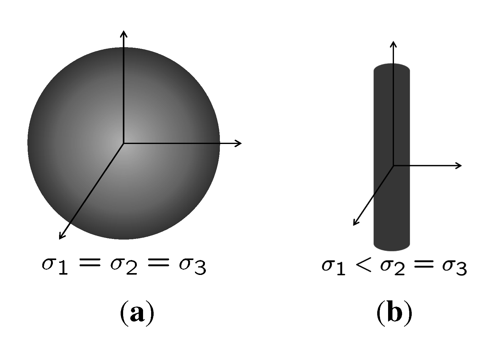
2.2. Moment-of-Inertia Filter

Nodules are often observed as globular regions, whereas blood vessels are as cylindrical regions. These two-type regions are distinguished based on the moment-of-inertia where voxel intensities are regarded as mass after applying the radial suppression filter. First, a gamma correction is applied to g(x, y, z) as follows:
g γ ( x y z ) = { g ( x y z ) } γ ,
where gγ(x, y, z) is the corrected image, and γ is the parameter of the gamma correction.
A moment-of-inertia tensor I is defined by
I = ( I x x I x y I x z I y x I y y I y z I z x I z y I z z ) ,
where
I x x = ( x , y , z ) K s p ( r f i x ) g γ ( x y z ) ( y 2 + z 2 ) ,
I y z = I z y = ( x , y , z ) K s p ( r f i x ) g γ ( x y z ) y z .
Ksp(rfix) is a domain of the spherical VOI whose radius is rfix.
Iyy, Izz, Ixy, Iyx, Ixz and Izx are defined in the same manner. From I, eigenvalues σ1(I), σ2(I) and σ3(I) (σ1(I) ≤ σ2(I) ≤ σ3(I)) and eigenvectors u1(I), u2(I) and u3(I) are calculated, where σi(I) corresponds to ui(I). If a candidate region is spherical, the three eigenvalues are the same as shown in Figure 5(a). If it is cylindrical, the eigenvalue corresponding to the longest direction of the region is smaller than the others as shown in Figure 5(b). A ratio between the eigenvalues σ 1 ( I ) σ 3 ( I ) is set into each voxel as the output of the filter as follows:
h ( x y z ) = σ 1 ( I ) σ 3 ( I ) .
The ratio represents an indicator to distinguish a nodule from the others. The larger the ratio is, the higher the confidence of a nodule is. Figure 6 shows the results obtained by applying the moment-of-inertia filter to the VOIs in Figure 4. In Figure 6(a), the nodule is successfully enhanced. In Figure 6(b), on the other hand, the blood vessel has excessively high values in its integument regions. They are compensated by use of the center displacement filter as described below.
Figure 5. Relationship of three eigenvalues of the moment-of-inertia filter. (a) globular; (b) cylindrical.
Algorithms 08 00209 g005
Figure 6. Results obtained by applying the moment-of-inertia filter. (a) nodule; (b) blood vessel.
Algorithms 08 00209 g006

2.3. Center Displacement Filter

The displacement d 2 between a VOI center and the gravity point of the voxel values in the VOI is calculated as follows:
d 2 = ( ( x , y , z ) K s p ( r f i x ) x g γ ( x , y , z ) ( x , y , z ) K s p ( r f i x ) g γ ( x , y , z ) ) 2 + ( ( x , y , z ) K s p ( r f i x ) y g γ ( x , y , z ) ( x , y , z ) K s p ( r f i x ) g γ ( x , y , z ) ) 2 + ( ( x , y , z ) K s p ( r f i x ) z g γ ( x , y , z ) ( x , y , z ) K s p ( r f i x ) g γ ( x , y , z ) ) 2 .
The output of the filter at each voxel is obtained by
q ( x , y , z ) = 1 d 2 + 1 h ( x , y , z ) .
This compensation enables to remain values in the middle parts of VOIs and suppress values in their periphery. Figure 7 shows the results obtained by applying the center displacement filter to the regions in Figure 6. High values remain at the center of the nodule in Figure 7(a), whereas the blood vessel is suppressed successfully in Figure 7(b).
Figure 7. Results of the center displacement filter. (a) nodule; (b) blood vessel
Algorithms 08 00209 g007

3. False positive reduction

3.1. Normalization of directions of intensity distributions

Several intensity distributions in VOIs are often approximately same to one another. For example, the three examples of VOIs in Figure 8 have almost same intensity distributions although their directions are different. In order to treat them in a unified manner, the VOIs are rotated three dimensionally by
X = RX ,
where R is a rotation matrix defined by
R = ( u 3 ( I ) | u 2 ( I ) | u 1 ( I ) ) T .
Figure 9 shows their rotation results. The major directions of the intensity distributions are unified to the z-axis.
Figure 8. Three examples of VOIs that have different directions of intensity distributions. (a) example 1; (b) example 2; (c) example 3. The first, second and third rows represent the upper slices, the slices of interest, and the lower slices, respectively.
Algorithms 08 00209 g008
Figure 9. Rotation results of the three examples in Figure 8 based on the eigenvalues of the intensity distributions. (a) example 1; (b) example 2; (c) example 3.
Algorithms 08 00209 g009

3.2. Appearance-Based k-means Clustering

The appearance-based two-step k-means clustering method is used to distinguish true nodules from false positives. The method constructs feature vectors composed of voxel values in the VOIs, and then applies the k-means clustering [23] to the feature vectors twice. The method is composed of the two phases as described below.

3.2.1. Training Phase

A cylindrical VOI is set on each voxel of interest. Here, we use such a cylindrical VOI instead of a spherical VOI because our preliminary experiences indicate that the cylindrical VOI is more accurate. Generally, the number of true positives (TPs) is much less than that of false positives. Our previous work [20] indicates that a training-based classification method performs better by taking the balance between TP numbers and FP numbers in its training phase. In order to compensate the lack of the TP numbers, pseudo TP VOIs are generated by translating actual VOIs to the four directions and then rotating them by 90 degrees in the azimuth and zenith directions. On the other hand, a certain number of FP VOIs are selected randomly. The actual TP VOIs, the pseudo TP VOIs and the selected FP VOIs are used as training data. Feature vectors are generated which are composed of voxel values in the VOIs. The first k-means clustering is performed based on the feature vectors. Let C 1 k denote the k-th cluster obtained by the first k-means clustering, and # T P 1 k the number of TPs in C 1 k . The feature vectors in the clusters whose #T P 1 k are not zero are extracted. Based on the extracted feature vectors, the k-means clustering is performed once again. Let C 2 k denote the k-th cluster obtained by the second k-means clustering. The moment-of-inertia filter is applied to the VOI that is generated by being inversely converted from the center vector of C 2 k . Eigenvalues, σ 1 and σ 3 , are calculated by applying the method described in Section 2.2 to the generated VOI, and then the eigenvalue ratio μ 2 k is calculated as follows:
μ 2 k = σ 1 σ 3 .

3.2.2. Testing Phase

Each query VOI is tested individually in this phase. First, the feature vector of a query VOI is generated in the same manner as the training phase. The correlation coefficient between the query vector and the gravity vector of each cluster C 1 k is calculated. The nearest cluster C 1 nearest is obtained based on the correlation coefficient. If #T P 1 nearest is zero, the query VOI is determined to be normal. Otherwise, the correlation coefficient η 2 k between the query VOI and the gravity vector of the cluster C 2 k is calculated. Then, the three nearest clusters C 2 nearest ( 1 ) , C 2 nearest ( 2 ) and C 2 nearest ( 3 ) are determined. The degree of abnormality eq of the query VOI is defined by
e q = s = 1 3 { μ 2 nearest ( s ) × η 2 nearest ( s ) + 1 2 } .
μ 2 k evaluates the degree of the globularity of a candidate region, and η 2 k evaluates the similarity between the query VOI and the cluster C 2 k . eq is larger as the region is more globular. Based on eq, the query VOI is determined to be abnormal or not.

4. Experimental Results

4.1. Experimental Conditions

The present method is applied to the Lung Image Database Consortium (LIDC) [19] dataset, where nodules are annotated by four radiologists. We select 50 CT scans that contain 104 nodules from 4 to 10 mm in diameter. 29 / 22 / 31 / 22 nodules are contained at the agreement levels 1 / 2 / 3 / 4, respectively. The slice numbers are from 102 to 371, and the pixel sizes are from 0.508 to 0.762 mm. The reconstruction intervals are from 0.75 to 3.0 mm. The parameters are set as follows: the radius of the spherical VOI at the initial detection phase is 15 voxels, and the radius and height of the cylindrical VOI at the false positive reduction phase are 10 voxels and 31 voxels, respectively. A feature vector used in the k-means clustering is generated from the values of voxels in the cylindrical VOI, and therefore the dimensionality of the feature vector is 9734. The numbers of clusters (i.e. the K values in the k-means clustering method) are set to be 15 / 20 / 25. 500 / 1000 / 1500 / 2000 FP VOIs are randomly selected at the training phase of the FP reduction. These parameters are determined experimentally.

4.2. Initial Nodule Detection

In the initial detection process, 99 nodules are detected successfully, and the number of false positives is 5,368 per scan. Most of false negatives (FNs) have low intensity less than −600 HU. One false negative has an irregular shape. Four of five FNs are at the agreement level 1 and the other is at the agreement level 3. Figure 10 shows the free-response receiver operating characteristic (FROC) curve of the initial detection of all the agreement levels. The numbers of FPs per scan at the TP ratios of 95.20% / 90.38% / 86.54% are 3,832 / 554 / 441, respectively. The FROC curves of individual agreement levels are represented in Figure 11. At the agreement level 1, the numbers of FPs per scan at the TP ratios of 86.21% / 79.31% are 1, 744 / 454, respectively, at the agreement level 2, those at the TP ratios of 95.45% / 90.91% are 1, 338 / 376, respectively. At the agreement level 3, the numbers of FPs per scan at the TP ratios of 96.77% / 90.32% are 502 / 344, respectively, at the agreement level 4, those at the TP ratios of 100% / 95.45% / 90.91% are 1090 / 696 / 556, respectively.
Figure 10. FROC curve of initial detection of all the agreement levels.
Algorithms 08 00209 g010
Figure 11. FROC curves of initial detection of individual agreement levels.
Algorithms 08 00209 g011

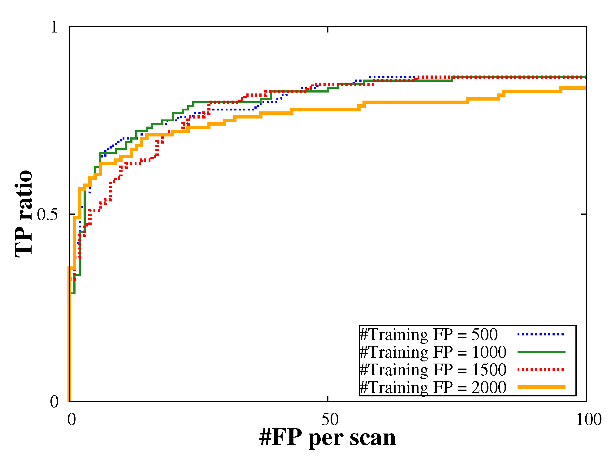
4.3. False Positive Reduction

At the false positive reduction process, we use the dataset at the TP ratio 90.38% of the initial detection. The dataset is divided into two subsets. Dataset A contains 13, 350 FPs and 50 TPs and Dataset B contains 14, 381 FPs and 44 TPs. The numbers of FNs at the datasets A and B are 5 and 5, respectively.
The FROC curves of the FP reduction are shown in Figure 12, where 500 / 1000 / 1500 / 2000 represent the numbers of the randomly selected FP VOIs for training. The numbers of the FPs per scan at the TP ratios of 84.6% are 48 / 52 / 47 / 110, respectively. Figure 13 shows the FROC curves of the 15 / 20 / 25 clusters at the 1500 FPs. The numbers of the FPs per scan at the TP ratios of 84.6% are 55 / 47 / 59, respectively.
Figure 12. FROC curves of individual FP numbers for training in FP reduction.
Algorithms 08 00209 g012
Figure 13. FROC curves of individual cluster numbers for training in FP reduction.
Algorithms 08 00209 g013

5.Discussion

Figure 14 shows examples of nodules detected by our proposed CAD system. Not only a typical nodule but also a juxtapleural nodule and an irregular nodule can be detected.
In the initial detection process, many false positives are generated due to the noises caused by the failure of the lung region extraction in the apex regions. Figure 15(a), (b) and (c) show an example of a CT slice including an apex region, the result of the lung region extraction, and the result of the initial detection, respectively. In Figure 15(b), several brighter spot regions remain as noises which cause the false positives in Figure 15(c).
The proposed filters cannot correctly recognize the nodules of irregular shapes. The LIDC dataset of the agreement levels 3 and 4 contain large nodules which tend to have irregular shapes. Figure 16(a) shows an example of a large nodule, (b) is the result of the moment-of-inertia filter and (c) is the result of the center displacement filter. In Figure 16(b), the center voxel of the VOI has high value, but it is mistakenly suppressed in Figure 16(c).
The performance of the k-means clustering strongly depends on the numbers of clusters as shown in Figure 12. In this paper, the numbers of clusters are determined experimentally.
Figure 14. Extracted nodules. (a) example 1; (b) example 2; (b) example 3.
Algorithms 08 00209 g014
Figure 15. The failure of the lung region extraction generates false positives. (a) Original slice section. (b) Extracted lung region. (c) Result of the initial detection.
Algorithms 08 00209 g015
Figure 16. An example of a false negative. (a) An example of a large nodule. (b) The result of the moment-of-inertia filter. (c) The result of the center displacement filter.
Algorithms 08 00209 g016
In the experiment of the FP reduction, we also employed one-step k-means clustering. The numbers of the FPs per scan at the TP ratio 84.6% are 97 / 153 / 103 / 95, respectively. The best performance is 95 FPs at the TP ratio of 84.6%. It implies that the two-step k-means clustering is more promising than the one-step k-means clustering.
In the experiment, we used the 50 CT scans that are selected from the LIDC dataset. Although the dataset contains more CT scans, we can apply the proposed method only to this subset. The main reason is that the method needs a lot of calculation time for the FP reduction process where the high-dimensional feature vectors are classified. In the future, we should apply the method to larger dataset by reducing the calculation time of the proposed method.
The FP reduction of the proposed method is not sufficient yet. The proposed method can be used as preprocessing for our previous methods[21,22] which can detect nodules more accurately. For further accuracy improvement, we should build a hybrid detection system by combining the proposed method with these methods in the future.

6. Conclusion

This paper proposed a detection method for pulmonary nodules by use of the radial suppression filter, the moment-of-inertia filter, and the center displacement filter followed by the two-step appearance-based k-means clustering. The proposed method is applied to 50 CT scans in the LIDC dataset. The number of FPs is 47 per scan at the TP ratio of 84.6%.

Author Contributions

Takanobu Yanagihara and Hotaka Takizawa built the proposed method; Takanobu Yanagihara designed and performed the experiments, and then analyzed the results; Takanobu Yanagihara and Hotaka Takizawa wrote the present paper.

Conflicts of Interest

The authors declare no conflict of interest.

References

  1. Yamamoto, S.; Tanaka, I.; Senda, M.; Tateno, Y.; Iinuma, T.; Matsumoto, T.; Matsumoto, M. Image Processing for Computer-Aided Diagnosis of Lung Cancer by CT(LSCT). Syst. Comput. Jpn. 1994, 25, 67–80. [Google Scholar] [CrossRef]
  2. Sone, S.; Matsumoto, T.; Honda, T.; Tsushima, K.; Takayama, F.; Hanaoka, T.; Kondo, R.; Haniuda, M. HRCT Features of Small Peripheral Lung Carcinomas Detected in a Low-dose CT Screening Program. Acad. Radiol. 2010, 17, 75–83. [Google Scholar] [CrossRef] [PubMed]
  3. Van Ginneken, B. Computer-Aided Diagnosis in Thoracic Computed Tomography. Imaging Decis. 2009, 12, 11–22. [Google Scholar] [CrossRef]
  4. Yamamoto, S.; Matsumoto, M.; Takano, Y.; Iinuma, T.; Matsumoto, T. Quoit Filter : A New Filter Based on Mathematical Morphology to Extract the Isolated Shadow, and Its Application to Automatic Detection of Lung Cancer in X-ray CT. In Proceedings of the 13th International Conference on Pattern Recognition, 25–29 August 1996; Volume 2, pp. 3–7.
  5. Messay, T.; Hardie, R.C.; Rogers, S.K. A new computationally efficient CAD system for pulmonary nodule detection in CT imagery. Med. Image Anal. 2010, 14, 390–406. [Google Scholar] [CrossRef] [PubMed]
  6. Lee, Y.; Hara, T.; Fujita, H.; Itoh, S.; Ishigaki, T. Automated Detection of Pulmonary Nodules in Helical CT Images Based on an Improved Template-Matching Technique. IEEE Trans. Med. Imaging 2001, 20, 595–604. [Google Scholar] [PubMed]
  7. Tan, M.; Bister, M.; Cornelis, J. A novel computer-aided lung nodule detection system for CT images. Med. Phys. 2011, 38, 5630–5645. [Google Scholar] [CrossRef] [PubMed]
  8. Stanley, K.O.; Miikkulainen, R. Evolving Neural Networks through Augmenting Topologies. Evolut. Comput. 2002, 10, 99–127. [Google Scholar] [CrossRef] [PubMed]
  9. Ozekes, S.; Osman, P. Computerized Lung Nodule Detection Using 3D Feature Extraction and Learning Based Algorithms. J. Med. Syst. 2010, 34, 185–194. [Google Scholar] [CrossRef] [PubMed]
  10. Lee, S.L.A.; Kouzani, A.Z.; Hu, E.J. Random forest based lung nodule classification aided by clustering. Comput. Med. Imaging Graph. 2010, 34, 535–542. [Google Scholar] [CrossRef] [PubMed]
  11. Choi, W.J.; Choi, T.S. Genetic programming-based feature transform and classification for the automatic detection of pulmonary nodules on computed tomography images. Inf. Sci. 2012, 212, 57–78. [Google Scholar] [CrossRef]
  12. Ye, X.; Lin, X.; Dehmeshki, J.; Slabaugh, G.; Beddoe, G. Shape-based computer-aided detection of lung nodules in thoracic CT images. IEEE Eng. Med. Biol. Soc. 2009, 56, 1810–1820. [Google Scholar]
  13. Brown, M.; McNitt-Gray, M.; Goldin, J.; Suh, R.; Sayre, J.; Aberle, D. Patient-specific models for lung nodule detection and surveillance in CT images. IEEE Trans. Med. Imaging 2001, 20, 1242–1250. [Google Scholar] [CrossRef] [PubMed]
  14. Osman, O.; Ozekes, S.; Ucan, O.N. Lung nodule diagnosis using 3D template matching. Comput. Biol. Med. 2007, 37, 1167–1172. [Google Scholar] [CrossRef] [PubMed]
  15. Paik, D.S.; Beaulieu, C.F.; Rubin, G.D.; Acar, B.; Jeffrey, J.; Yee, J.; Dey, J.; Napel, S. Surface normal overlap: A computer-aided detection algorithm with application to colonic polyps and lung nodules in helical CT. IEEE Trans. Med. Imaging 2004, 23, 661–675. [Google Scholar] [CrossRef] [PubMed]
  16. Suarez-Cuenca, J.; Tahoces, P.; Souto, M.; Lado, M.; Remy-Jardin, M.; Remy, J.; Vidal, J.J. Application of the iris filter for automatic detection of pulmonary nodules on computed tomography images. Comput. Biol. Med. 2009, 39, 921–933. [Google Scholar] [CrossRef] [PubMed]
  17. Golosio, B.; Masala, G.L.; Piccioli, A.; Oliva, P.; Carpinelli, M.; Cataldo, R.; Cerello, P.; DeCarlo, F.; Falaschi, F.; Fantacci, M.E.; et al. A novel multithreshold method for nodule detection in lung CT. Med. Phys. 2009, 36, 3607–3618. [Google Scholar] [CrossRef] [PubMed]
  18. Suzuki, K.; Armato, S.G., 3rd; Li, F.; Sone, S.; Doi, K. Massive training artificial neural network (MTANN) for reduction of false positives in computerized detection of lung nodules in low-dose computed tomography. Med. Phys. 2003, 30, 1602–1617. [Google Scholar] [CrossRef] [PubMed]
  19. Armato, S.G.; McLennan, G.; McNitt-Gray, M.F.; Meyer, C.R.; Yankelevitz, D.; Aberle, D.R.; Henschke, C.I.; Hoffman, E.A.; Kazerooni, E.A.; MacMahon, H.; et al. Lung image database consortium: Developing a resource for the medical imaging research community. Radiology 2004, 232, 739–748. [Google Scholar] [CrossRef] [PubMed]
  20. Takizawa, H.; Nishizako, H. Lung Cancer Detection from X-ray CT Scans Using Discriminant Filters and View-based Support Vector Machine. J. Insti. Image Electron. Eng. Jpn. 2011, 40, 59–66. [Google Scholar]
  21. Fukano, G.; Nakamura, Y.; Takizawa, H.; Mizuno, S.; Yamamoto, S.; Doi, K.; Katsuragawa, S.; Matsumoto, T.; Tateno, Y.; Iinuma, T. Eigen Image Recognition of Pulmonary Nodules from Thoracic CT Images by Use of Subspace Method. IEICE Trans. Inf. Syst. 2005, E88-D-II, 1273–1283. [Google Scholar] [CrossRef]
  22. Takizawa, H.; Yamamoto, S.; Shiina, T. Recognition of Pulmonary Nodules in Thoracic CT Scans Using 3-D Deformable Object Models of Different Classes. Algorithms 2010, 3, 125–144. [Google Scholar] [CrossRef]
  23. Forsyth, D.A.; Ponce, J. Computer Vision: A Modern Approach; Prentice Hall: Upper Saddle River, NJ, USA, 2003. [Google Scholar]

