An Adaptive Spectral Clustering Algorithm Based on the Importance of Shared Nearest Neighbors

Xiaoqi He; Sheng Zhang; Yangguang Liu

doi:10.3390/a8020177

,

and

¹

School of Information Science and Engineering, Ningbo Institute of Technology, Zhejiang University, Ningbo 315100, China

²

School of Electronics and Information Engineering, Taiyuan University of Science and Technology, Taiyuan 030024, China

^*

Author to whom correspondence should be addressed.

Algorithms2015, 8(2), 177-189;https://doi.org/10.3390/a8020177

Version Notes

Order Reprints

Abstract

The construction of a similarity matrix is one significant step for the spectral clustering algorithm; while the Gaussian kernel function is one of the most common measures for constructing the similarity matrix. However, with a fixed scaling parameter, the similarity between two data points is not adaptive and appropriate for multi-scale datasets. In this paper, through quantitating the value of the importance for each vertex of the similarity graph, the Gaussian kernel function is scaled, and an adaptive Gaussian kernel similarity measure is proposed. Then, an adaptive spectral clustering algorithm is gotten based on the importance of shared nearest neighbors. The idea is that the greater the importance of the shared neighbors between two vertexes, the more possible it is that these two vertexes belong to the same cluster; and the importance value of the shared neighbors is obtained with an iterative method, which considers both the local structural information and the distance similarity information, so as to improve the algorithm’s performance. Experimental results on different datasets show that our spectral clustering algorithm outperforms the other spectral clustering algorithms, such as the self-tuning spectral clustering and the adaptive spectral clustering based on shared nearest neighbors in clustering accuracy on most datasets.

Keywords:

spectral clustering; similarity measures; Gaussian kernel function; importance of nearest neighbors

1. Introduction

Over the past several decades, the spectral clustering algorithm has attracted a great amount of attention in the field of pattern recognition and become a research hot spot [1]. It has the feature that it does not assume for the global structure of the dataset, but directly finds the global optimal solution on a relaxed continuous domain through decomposition of the Laplacian matrix of the graph. Therefore, it is simple to implement and is solved efficiently by standard linear algebra, so that it often outperforms the traditional clustering algorithms, such as the k-means algorithm [2].

Spectral clustering consists of one significant step in which a similarity matrix (graph) with a kind of similarity measure should be constructed. The main goal of constructing the similarity matrix is to model the local neighborhood relationships between the data vertexes. A good similarity matrix is greatly responsible for the performance of spectral clustering algorithms [3].

The Gaussian kernel function is one of the most common similarity measures for spectral clustering, in which a scaling parameter σ controls the speed of the similarity falling off with the distance between the vertexes. Though its computation is simple and the results of the positive definite similarity matrix can simplify the analysis of eigenvalues, it does not work well on some complex datasets, e.g., a multi-scale dataset [4]. Moreover, the scaling parameter σ is specified manually, so that the similarity between two vertexes is only determined by their Euclidean distance.

In recent years, there have appeared some new construction methods of the similarity matrix. Fischer et al. [5] proposed a path-based clustering algorithm for texture segmentation. Their algorithm utilizes a connectedness criterion, which considers two objects as similar if there exists a mediating intra-cluster path without an edge with large cost, and it is used for spectral clustering. The construction method mainly combines the Gaussian kernel function with the shortest path, which is effective on some datasets, but sensitive to outliers. Chang et al. [6] utilized the idea of M-estimation and developed a robust path-based spectral clustering method by defining a robust path-based similarity measure for spectral clustering, which can effectively reduce the influence of outliers. Yang et al. defined adjustable line segment lengths, which can squeeze the distances in high density regions, but widen them in low density regions, and proposed a density-sensitive distance similarity function for the spectral clustering [7]. Assuming that each data point can be linearly reconstructed from its local neighborhoods, Gong et al. utilized the contributions between different vertexes in neighborhoods through n standard quadratic programming to get the similarity, rather than Gaussian kernel function, and to get a better cluster performance [8]. Zhang et al. adopted multiple methods of vector similarity measurement to produce diverse similarity matrices to get a new similarity matrix through particle swarm optimization and proposed a new similarity measure [9]. The construction methods utilized the idea of ensemble learning, which is helpful to improve the cluster performance. Cao et al. utilized the maximum flow to be computed as the new similarity between data points, which carried the global and local relations between data and worked well on a dataset with a nonlinear and elongated structure [10].

The multi-scaled self-tuned kernel function for spectral clustering is also a significant research direction. Erdal Yenialp et al. proposed a multi-scale density-based spatial clustering algorithm with noise. The proposed algorithm represents the images in multiple scales by using Gaussian smoothing functions and evaluates a density matrix for each scale. The density matrices in each scale are then fused to capture salient features in each scale. The developed algorithm does not include a training phase, so computationally-efficient solutions could be reached to segment the region-of-interest [11]. Hsieh Fushing et al. developed a new methodology, called data cloud geometry-tree, which derived from the empirical similarity measurements a hierarchy of clustering configurations that captures the geometric structure of the data, and had a built-in mechanism for self-correcting clustering membership to multi-scale clustering, which provided a better quantification of the multi-scale geometric structures of the data [12]. Raghvendra et al. created a parameter-free kernel spectral clustering model and exploited the structure of the projections in the eigenspace to automatically identify the number of clusters, which showed the efficiency for large-scale complex networks [13]. Manor et al. introduced a self-tuning scaling parameter for the Gaussian kernel function, and on that basis, Li et al. introduced a parameter for the shared nearest neighbors self-tuning Gaussian kernel function and proposed an adaptive spectral clustering algorithm based on the shared nearest neighbors. This algorithm exploited the information about local density embedded in the shared nearest neighbors, thereby learning the implicit information of the cluster’s structure and improving the algorithm’s performance [14,15].

Due to the non-homogeneous of the network topology, each node in the network is of different importance. The similarity of two vertices relates not only to the number of neighbors shared, but also closely to the importance of the shared neighbor vertices. In a graph, the importance of a vertex is related to the vertex’s out-degree, in-degree and neighboring vertexes’ importance. The greater the importance of the shared neighbors between two vertexes, the more possible it is that these two vertexes belong to the same cluster. Blondel et al. introduced hubs and authorities based on the idea of characterizing the most important vertices in a graph representing the connections between vertices [16]. From an implicit relation, an “authority score” and a “hub score” to each vertex of a given graph can be obtained as the limit of a converging iterative process, which can be used to represent the importance of the vertices [17].

In this paper, we propose the importance of a shared nearest neighbors-based similarity measure for constructing the similarity matrix, originating from the idea of “authority score” and “hub score”. In this measure, we first find the importance of every vertex through the limitation of a converging iterative process and then look for the maximal importance in shared nearest neighbors between each of two vertices. The greater the maximal importance, the more similar the two vertices are. Therefore, we can get structure information between every two vertices and then utilize this information to self-tune the Gaussian kernel function. Finally, we get the similarity measure based on the importance of shared nearest neighbors.

The rest of this paper is organized as follows. In Section 2, we give a brief outline of similarity graphs. In Section 3, we propose a new similarity measure and apply it to the construction of the similarity matrix. In Section 4, we present the experiment results for the proposed algorithm on some datasets, followed by the concluding remarks given in Section 5.

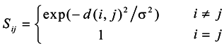
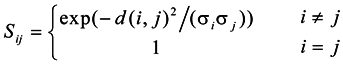
2. Similarity Graphs

Given a set of data points x₁,…,x_n and some notion of similarity s_ij ≥ 0 between all pairs of data points x_i and x_j, the intuitive goal of clustering is to divide the data points into several groups, so that points in the same group are similar and points in different groups are dissimilar to each other. If we do not have more information than similarities between data points, a nice way of representing the data is in the form of the similarity graph G = (V,E). Each vertex v_i in this graph represents a data point x_i. Two vertices are connected if the similarity s_ijbetween the corresponding data points x_iand x_j is positive or larger than a certain threshold and the edge is weighted by s_ij. The problem of clustering can now be reformulated by using the similarity graph: we want to find a partition of the graph so that the edges between different groups have very low weights and the edges within a group have high weights.

The goal of constructing similarity graphs is to model the local neighborhood relationships between the data points. As far as we know, the Gaussian kernel function is still an important construction method; and the important feature of the Gaussian kernel function is that the construction form is based on the Gaussian kernel model, which can be defined as Equation (1).

(1)

Where, the d(i,j) is the Euclidean distance between x_i and x_j, and σ is the kernel parameter, which is a fixed parameter and cannot vary with the change of the surroundings. Zelnik-Manor et al. proposed a local scale parameter σ_i for each point to replace the fixed parameter σ[14], which allows the similarity self-tuning capability. Usually, σ_i = d(x_i, x_m), where x_m is the m-th closest neighbor of the point x_i, and the similarity function is defined as Equation (2).

(2)

Jarvis et al. proposed a conception of the shared nearest neighbor, which is used to characterize the local density of different vertices [18]. Supposing the closest kd nearest neighbors of point x_ican construct a set N(x_i) and point x_j can construct a set N(x_j), then the shared neighbor vertexes between x_i and x_j are defined as Equation (3).

(3)

Li et al. assumed that vertexes in the same manifold have a higher similarity and a higher local density region than those in different manifolds. They used the number of the shared nearest neighbors to characterize the similarity between vertex x_i and x_j [15]. The construct similarity function is defined as Equation (4).

(4)

According to this method, the similarity between two vertexes is higher if there are more common shared nearest neighbors. Due to the non-homogeneity of the network topology, the importance of each node in the network is different, and the similarity of two vertices relates to not only the number of neighbors shared, but also closely to the importance of the shared neighbor vertices.

3. Similarity Matrix Based on the Importance of Shared Nearest Neighbors

3.1. The Importance of Node

Some efficient web searching engines are often based on the idea of characterizing the most important vertices in a graph representing the connections or links between pages on the web, such as Google. Because the linkages between pages can be interpreted as interrelated and mutually supportive between pages, the importance of a page can be determined according to the linkages. Kleinberg et al. proposed a similar method to identify in a set of pages relevant to a query search the subset of pages that are good hubs or the subset of pages that are good authorities [17]. Good hubs are pages that point to good authorities, and good authorities are pages that are pointed to by good hubs. From these implicit relations, Kleinberg derived an iterative method that assigns an “authority score” and a “hub score” to every vertex of a given graph.

Given a graph G = (V,E) with vertex set V and with edge set E, let h_i and a_i be the hub and authority scores of vertex i. The hub score of vertex i is set equal to the sum of the authority scores of all vertices pointed to by i, and similarly, the authority score of vertex i is the set equal to the sum of the hub scores of all vertices pointing to i. The scores of h_i and a_i can be calculated as Equation (5).

(5)

Let these scores be initialized by some positive values and then update them simultaneously for all vertices; the “authority score” and “hub score” can be obtained as a limit of a converging iterative process according to Equation (6):

(6)

Where, B is the matrix whose entry (i,j) is equal to the number of edges between the vertices i and j in G (the adjacency matrix of G). Blondel et al. has proven that in the initial condition Algorithms 08 00177 i007

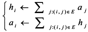
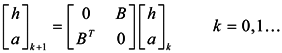
; Equation (4) will converge when the number of iterations is odd or even times, respectively [16]. When getting the “authority score” and a “hub score” for every vertex, the score of vertex importance can be calculated as Im = (h+a). Obviously, the importance of one vertex is related to the vertex’s out-degree, in-degree and neighboring vertexes’ importance, to represent the structure and properties characteristics of the network. Similarly, we can utilize the score of vertex importance to construct a similarity matrix in graph G.

3.2. Similarity Matrix Based on the Importance of Shared Nearest Neighbors

In this section, we propose a new similarity matrix construction method based on the importance of shared nearest neighbors. There exists a local high density area in the same cluster, and it can be expressed by the numbers of shared nearest neighbors. Obviously, the role of every node in the local area is different, so in the shared nearest neighbors, the more important the role of one node, the more impact of the vertexes for the graph. Though we cannot give an explicit expression of the role of each node, we hold the opinion that the importance of one vertex is helpful to find some potential “critical nodes” and reflects the global and local importance of the node. The greater the importance of the node, the more it is close to the center of network. In the shared nearest neighbors between two vertices, the greater the neighbor’s scores are, the more similar the two vertices are. On the basis of this idea, a new kind of similarity measure based on the importance of shared nearest neighbors is proposed. The steps of computing the similarity matrix is described in Table 1.

Assume the matrix SNEW to be the similarity matrix based on the importance of shared nearest neighbors. We can derive that the construction method is similar to the adaptive Gaussian kernel function based on shared nearest neighbors, SNN, while the difference is that the maximal importance in shared nearest neighbor vertexes is used to replace the number of shared neighbor vertexes. In fact, through adjusting different parameters, SNEW can become the Gaussian kernel function described in self-tuning spectral clustering or SNN. Meanwhile, it is worth noting that there are many choices of shared neighbors, but we choose the vertex with the maximal importance in shared nearest neighbors, not only because the importance of the vertex can express the structural information of global graph, but also the maximal importance can affect the similarity between vertexes in the local structure of the graph. Nevertheless, the shared nearest neighbors reflect the local density information, so the matrix SNEW has considered both structure attributes of the graph and the local density information, so the measure can represent the inner link between vertexes more reasonably.

Table 1. The algorithm of similarity matrix based on the importance of shared nearest neighbors.

**Table 1.** The algorithm of similarity matrix based on the importance of shared nearest neighbors.
Similarity matrix based on the importance of shared nearest neighbors:
Input: n data vertexes, ; Output: similarity matrix SNEW.
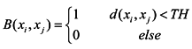
Step1. Construct an adjacency matrix B of graph G according to Equation (7). The construction of adjacency matrix B can be similar to the ɛ-neighborhood technique. (7) Where, the d(x_i, x_j) is the Euclidean distance between x_i and x_j, and the TH is an ordinary threshold about Euclidean distance d and is set as the mean value of d.
Step2. Set , and iterate an even number of times with Equation (4). Stop upon convergence and get the importance score of every vertex .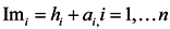
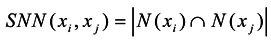
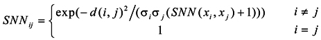
Step3. Look for shared nearest neighbor vertexes between x_i and x_j, and find the maximal importance in shared nearest neighbors; set it as: $S N N_{\max} Im (x_{i}, x_{j}) \dots i = 1, \dots, n; j = 1, \dots, n$ ;
Step4. Get a new kind of similarity matrix by Equation (8): $S N E W_{i j} = {\begin{array}{c} \exp (- d {(x_{i}, x_{j})}^{2} / ((1 + α S N N_{\max} Im) σ_{i} σ_{j})) & i \neq j \\ 1 & i = j \end{array}$ (8) Where α is a regulation parameter, and α > 0; add 1 to make sure that it not divided by zero.

3.3. An Improved Adaptive Spectral Clustering Algorithm

Spectral clustering is a clustering method that is based on graph theory and uses the feature vectors of a data similarity matrix to make the clustering. It can identify a data space of arbitrary shape and converge to the global optimal solution.

Let us consider a set V of N data points, or vertices. We write S_ij for the similarity between the i-th and the j-th data point, and S = S_ij for the N × N similarity matrix. Let us define the degrees D_ij of vertex i ∈ V by Equation (9):

D_{i i} = \sum_{j \in V} S_{i j}

(9)

Without loss of generality, we assume that all vertices have non-zero degrees. Then, we write D = (D_ij) for the N × N diagonal matrix.

One spectral clustering technique, commonly used for image segmentation, is the normalized cuts algorithm or Shi-Malik algorithm introduced by Shi and Malik [19]. It partitions points into k sets,

{A_{1}, A_{2}, \dots, A_{k}}

, based on the eigenvectors v corresponding to the first k biggest eigenvalues of the symmetric normalized Laplacian defined as,

L^{n o r m} : = D^{- 1 / 2} S D^{- 1 / 2}

.

We introduce the proposed similarity matrix SNEW to the standard spectral clustering and then get a new adaptive spectral clustering algorithm based on the importance of shared nearest neighbors. The steps of improved adaptive spectral clustering algorithm is described in Table 2:

Table 2. Adaptive spectral clustering algorithm based on the importance of shared nearest neighbors.

**Table 2.** Adaptive spectral clustering algorithm based on the importance of shared nearest neighbors.
Adaptive spectral clustering algorithm based on the importance of shared nearest neighbors:
Input: n data vertexes: $X = {x_{1}, \dots, x_{n}} \in R^{d}$ , clustering number: K: Output: K clusters, ${A_{1}, \dots, A_{n}}$
Step1. Get the similarity matrix SNEW according to the calculation steps of the Table1;
Step2. Define D to be the diagonal matrix, where $D_{i i} = \sum_{i = 1}^{n} S N E W_{i j}$ , and compute the Laplacian matrix $L = D^{- 1 / 2} (S N E W) D^{- 1 / 2}$ ;
Step3.Compute the first K largest eigenvalues of the Laplacian matrix and their corresponding eigenvectors $v_{1}, v_{2}, \dots, v_{k}$ ; construct a matrix $U = {v_{1}, v_{2}, \dots, v_{k}}$ ;
Step4. Construct the matrix Y by normalizing each row in U, where $Y_{i j} = U_{i j} / \sqrt{(\sum_{j} u_{i j}^{2})}$ ;
Step5. Treat each row of Y as a vertex in space R^k and cluster them into K clusters via k-means or other clustering algorithms for the ultimate clustering results, ${A_{1}, \dots, A_{n}}$ .

4. Experiments

To evaluate the performance of the adaptive spectral clustering algorithm based on the importance of shared nearest neighbors (SNNISC), experiments are conducted on the synthetic, UCI Machine Learning Repository (UCI) and the MNIST database of handwritten digits (MNIST) in comparison with the other two spectral clustering algorithms, the self-tuning spectral clustering (SSC) [14] and the adaptive spectral clustering based on shared nearest neighbors (SNNSC) [15], respectively.

4.1. Evaluation Metric

Given a dataset with n samples, clustering is classified as a relationship between samples; the samples are divided into the same clusters, or different clusters. In following experiments, we adopt the adjusted Rand index (ARI) as the performance metric.

The adjusted Rand index assumes the generalized hyper geometric distribution as the model of randomness, i.e., the different partitions of the objects are picked at random, such that the number of objects in the partitions to compare is fixed. The general form of ARI can be simplified as Equation (10).

A R I = \frac{\sum_{i, j} (\begin{matrix} n_{i j} \\ 2 \end{matrix}) - [\sum_{i} (\begin{matrix} n_{i .} \\ 2 \end{matrix}) \sum_{j} (\begin{matrix} n_{. j} \\ 2 \end{matrix})] / (\begin{matrix} n \\ 2 \end{matrix})}{\frac{1}{2} [\sum_{i} (\begin{matrix} n_{i .} \\ 2 \end{matrix}) + \sum_{j} (\begin{matrix} n_{. j} \\ 2 \end{matrix})] - [\sum_{i} (\begin{matrix} n_{i .} \\ 2 \end{matrix}) \sum_{j} (\begin{matrix} n_{. j} \\ 2 \end{matrix})] / (\begin{matrix} n \\ 2 \end{matrix})}

(10)

Where, the n_ij is the number of objects that are both in different partitions; the n_i and n_j are the number of objects in different clusters, respectively. The ARI can take on a wider range of values between zero and one, with the increasing sensitivity of the index.

4.2. Parameter Settings

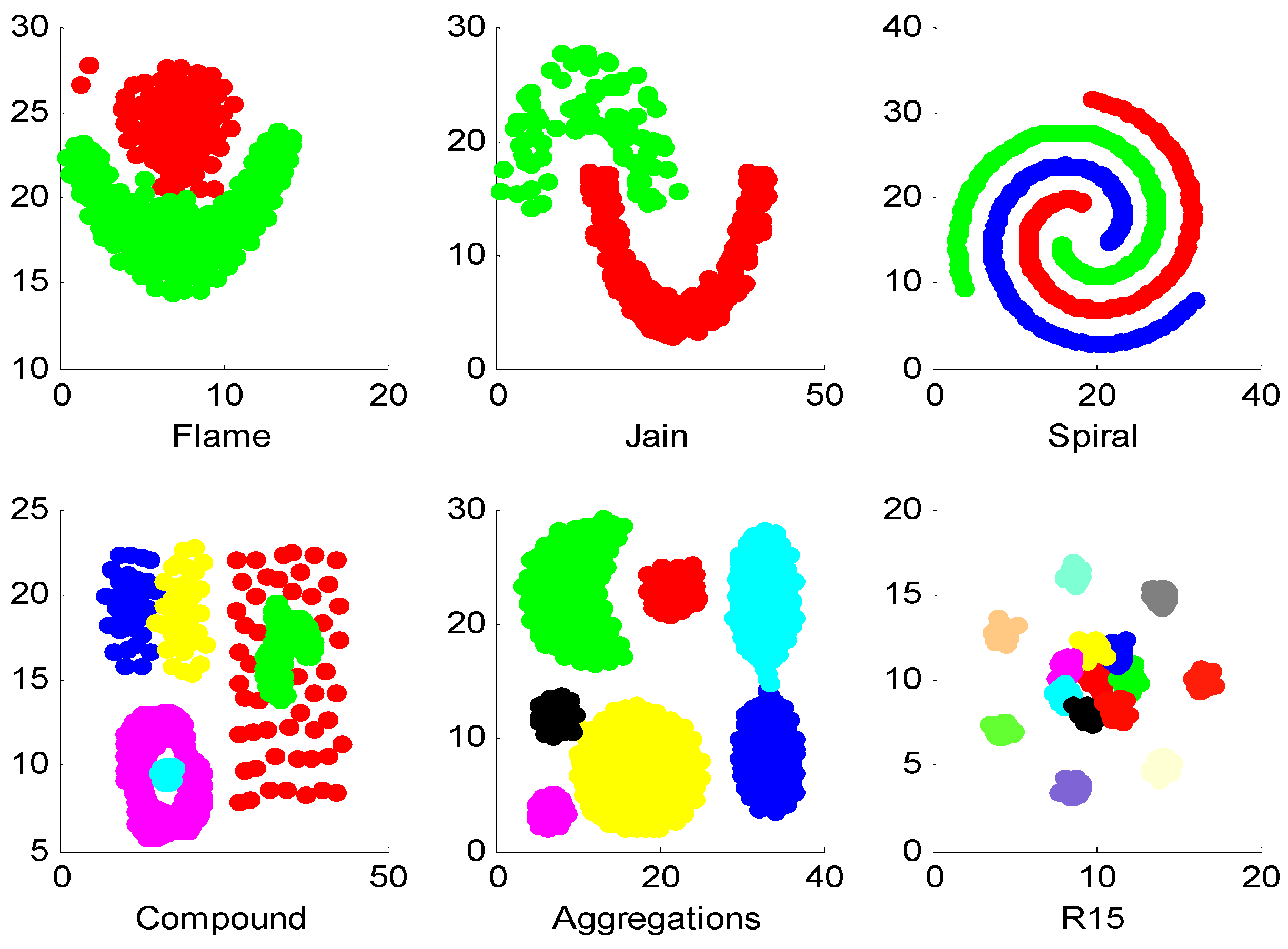
In SSC, a similar local scale parameter σ_i is used and is actually computed as its distance to the M-th neighbor. In our experiments, the range of M is [2,20], and the one that gets the best ARI values is used. SNNSC involves the number of shared nearest neighbors’ parameter kd. The range of kd is [5,50], and the one that gets the best ARI value is picked. The range of α is [10,20]. The value of TH is set as the mean value of Euclidean distance of all vertexes.

4.3. Experiments on Synthetic Datasets

As shown in Figure 1, six synthetic datasets [20] with different structure are used in the experiments, and the results are shown in Table 3.

Figure 1. Synthetic datasets.

This example is used to test the ability of identifying different structures on synthetic datasets. In Table 3, the average value is used to show the average performance of algorithms on different datasets, and the best value is marked by boldface. It can be seen from the Table 3 that SSC, SNNSC and SNNISC get similar results on all the datasets (about 97%, except on the forth dataset), which indicates that the proposed similarity measure can effectively identify different synthetic datasets.

Table 3. The results of adjusted Rand index (ARI) on synthetic datasets. SSC, self-tuning spectral clustering; SNNSC, spectral clustering based on shared nearest neighbors, SNNISC, the adaptive spectral clustering algorithm based on the importance of shared nearest neighbors.

**Table 3.** The results of adjusted Rand index (ARI) on synthetic datasets. SSC, self-tuning spectral clustering; SNNSC, spectral clustering based on shared nearest neighbors, SNNISC, the adaptive spectral clustering algorithm based on the importance of shared nearest neighbors.
Datasets	Spectral Clustering Algorithm
Datasets	SSC	SNNSC	SNNISC
Flame	0.95	0.97	0.97
Jain	1	1	1
Spiral	1	1	1
Compound	0.54	0.54	0.54
Aggregations	0.97	0.98	0.97
R15	0.99	0.99	0.99

4.4. Experiments on UCI Datasets

To test the performance of SNNISC further, eight real-word datasets are adopted from UCI datasets about classification and clustering [21,22,23,24,25,26,27,28,29], and the results are shown in Table 4. From the boldface in the Table 4, we observe that the clustering performance of SNNISC is superior to SSC and SNNSC on four datasets in addition to “Breast Tissue” and “Data Bank”. In particular, for the dataset “Iris”, one cluster is linearly separable from the other two nonlinearly clusters, which is challenging for clustering algorithms. Although the ARI value of SSC and SNNSC can reach to about 83%, SNNISC can achieve 92%. On dataset “Seeds”, SNNISC, SNNSC and SSC get the same ARI value (71%).

On dataset “Glass”, the ARI value of SNNISC (24%) is less than SSC (27%), but better than SNNSC (23%). Meanwhile, it can be found that SNNISC is more stable, which is just less than the best result between 0.2%~0.3%.Therefore, we conclude that the SNNISC can improve the performance of the spectral clustering algorithm.

Table 4. The results of ARI on the UCI Machine Learning Repository.

**Table 4.** The results of ARI on the UCI Machine Learning Repository.
Datasets	Spectral Clustering Algorithm
Datasets	SSC	SNNSC	SNNISC
Iris	0.82	0.83	0.92
Ionosphere	0.22	0.22	0.23
Breast Tissue	0.20	0.22	0.18
Banknote	0.29	0.58	0.56
Seeds	0.71	0.71	0.71
Fertility	0.11	0.11	0.12
Libras	0.37	0.37	0.38
Glass	0.27	0.23	0.24

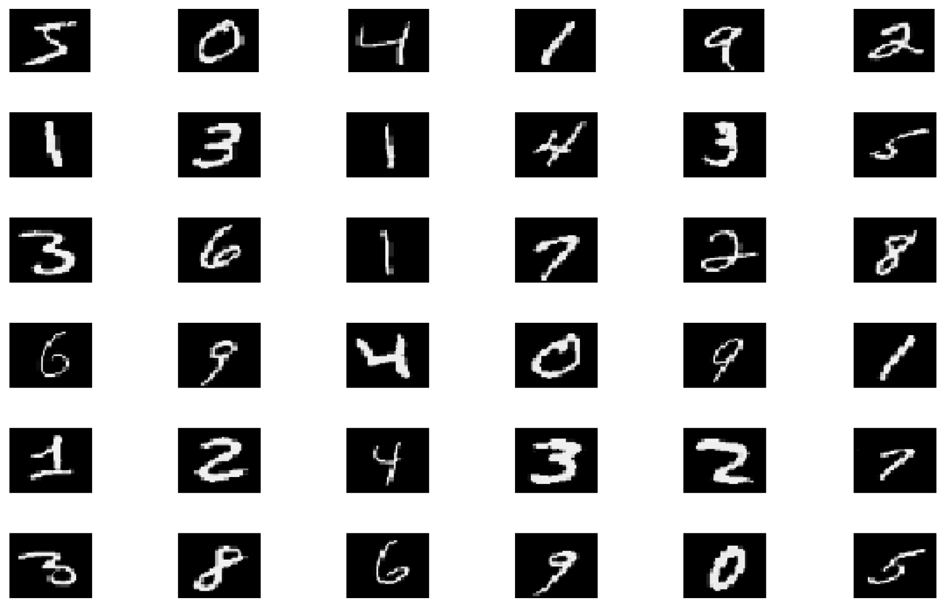
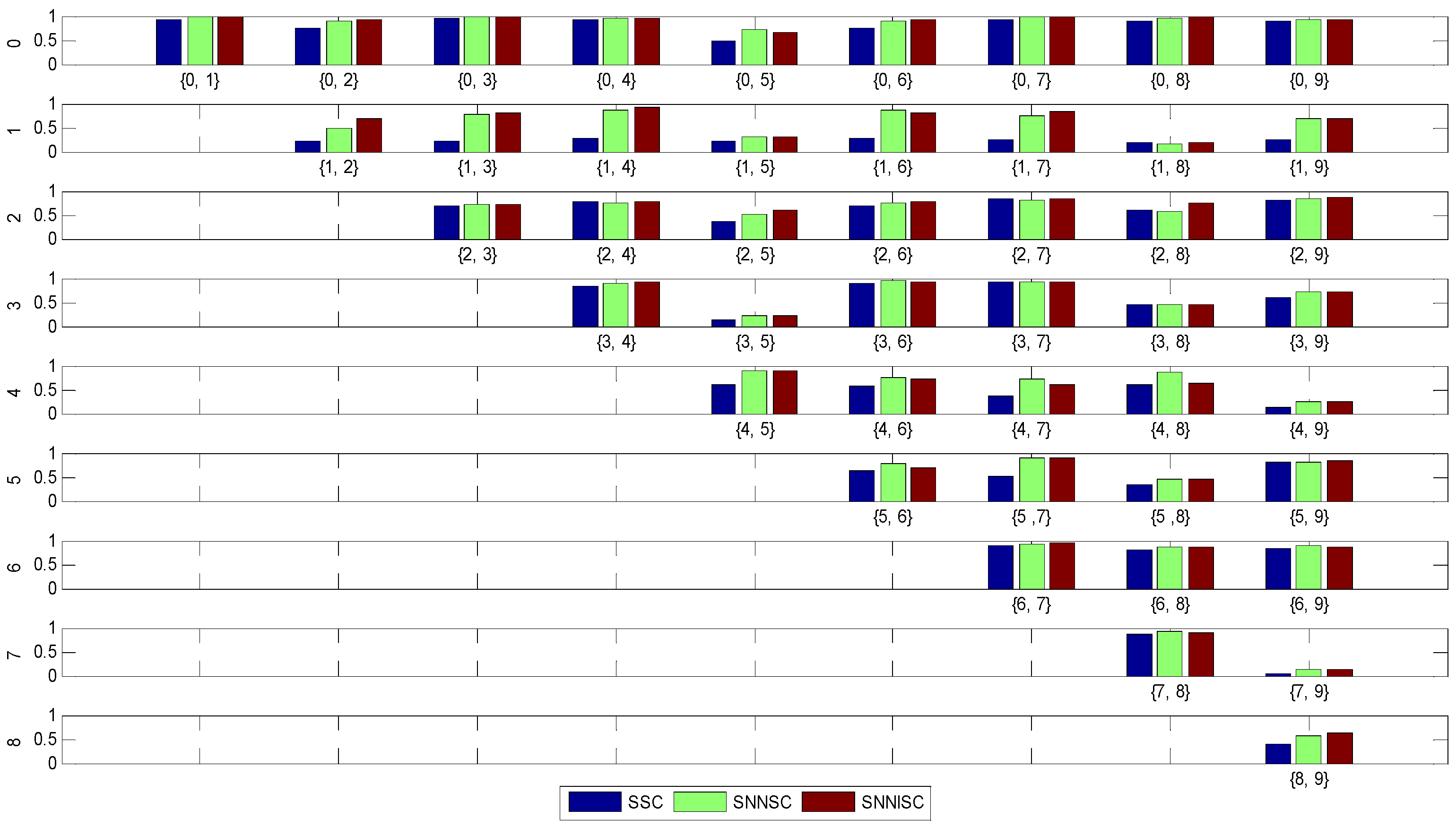
4.5. Experiments on MNIST Datasets

The MNIST dataset of handwritten digits [30] contains 10 digits with a total of 50,000 examples (Figure 2). Every example is a 28 × 28 grayscale image, and the dimension is 784. To obtain a comparable result, in our experiments, the first 900 examples are used. Each pair of the digits is used for clustering, with a total of 45 tests. Figure3 shows the results. The mean value and standard deviation of ARIs of different methods on the 45 tests are shown in Table 5.

From Figure 3, we observe that SNNISC and SNNSC get a similar ARI value in some tests, but in most cases (about 73% of tests), SNNISC is superior to SNNSC and SSC. From Table 5, we find that the mean value of SNNISC (74%) is better than SNNSC (73%) and SSC (59%), and the standard deviation of SNNISC (23%) is less than SNNSC (24%) and SSC (28%). This shows that the proposed method has the best performance and is robust for most data.

Figure 2. Some examples from the MNIST datasets of handwritten digits.

Figure 3. The ARI results of 45 tests on all pairs of 10 digits.

Table 5. Mean and standard deviation of ARIs of different spectral clustering methods.

**Table 5.** Mean and standard deviation of ARIs of different spectral clustering methods.
Clustering Results	Spectral Clustering Algorithm
Clustering Results	SSC	SNNSC	SNNISC
Mean	0.59	0.73	0.74
Standard deviation	0.28	0.24	0.23

5. Conclusions

The construction of a similarity matrix is important for spectral clustering algorithms. In this paper, we propose an adaptive Gaussian kernel similarity measure and its corresponding spectral clustering algorithm. The algorithm introduces the importance of nodes from the complex networks and uses an iterative method to get the numerical value of the importance of different vertexes to scale the Gaussian kernel function. The new measure exploits the structural information of the neighborhood and local density information and reflects the idea that the greater the importance of the shared neighbors between two vertexes is, the more likely these two vertexes are to belong to the same cluster. From the experiments on different datasets, we observe that it achieves improvements over the self-tuning spectral clustering algorithm and the adaptive spectral clustering algorithm based on shared nearest neighbors on most datasets and that it is less sensitive to the parameters. In this paper, we mainly consider the impact on the similarity of the vertex with maximal importance in shared nearest neighbors, and one important future work is to investigate the impact of other vertexes in shared nearest neighbors.

Acknowledgments

This work was supported by the Ningbo Natural Science Foundation of China, Grant No. 2011A610177, and partially supported by the Zhejiang Province Education Department Science Research project, Grant No. Y201327368.

Author Contributions

The work presented here was carried out in collaboration between all authors. Xiaoqi He designed the methods, and Yangguang Liu defined the research theme. Sheng Zhang carried out experiments, analyzed the data and interpreted the results. Yangguang Liu provided suggestions and comments on the manuscript and polished up the language in the paper. All authors have contributed to reading and approved the manuscript.

Conflicts of Interest

The authors declare no conflict of interest.

References

Xiaoyan, C.; Guanzhong, D.; Libing, Y. Survey on Spectral Clustering Algorithm. Comput. Sci. 2008, 35, 14–18. [Google Scholar]
Von Luxburg, U. A tutorial on spectral clustering. Stat. Comput. 2007, 17, 395–416. [Google Scholar] [CrossRef]
Jordan, F.; Bach, F. Learning spectral clustering. Adv. Neural Inf. Process. Syst. 2004, 16, 305–312. [Google Scholar]
Ng, A.Y.; Jordan, M.I.; Weiss, Y. On Spectral Clustering: Analysis and an algorithm. Proc. Adv. Neural Inf. Process. Syst. 2001, 14, 849–856. [Google Scholar]
Fischer, B.; Buhmann, J.M. Path-based clustering for grouping of smooth curves and texture segmentation. IEEE Trans. Pattern Anal. Mach. Intell. 2003, 25, 513–518. [Google Scholar] [CrossRef]
Chang, H.; Yeung, D.Y. Robust path-based spectral clustering. Pattern Recognit. 2008, 41, 191–203. [Google Scholar] [CrossRef]
Yang, P.; Zhu, Q.; Huang, B. Spectral clustering with density sensitive similarity function. Knowl.-Based Syst. 2011, 24, 621–628. [Google Scholar] [CrossRef]
Gong, Y.C.; Chen, C. Locality spectral clustering. In AI 2008: Advances in Artificial Intelligence; Springer: Berlin; Heidelberg, Germany, 2008; pp. 348–354. [Google Scholar]
Zhang, T.; Liu, B. Spectral Clustering Ensemble Based on Synthetic Similarity. In Proceedings of the 2011 Fourth International Symposium on ComputationalIntelligence and Design (ISCID), Hangzhou, China, 28–30 October 2011; Volume 2, pp. 252–255.
Cao, J.; Chen, P.; Zheng, Y.; Dao, Q. A Max-Flow-Based Similarity Measure for Spectral Clustering. ETRI J. 2013, 35, 311–320. [Google Scholar] [CrossRef]
Yenialp, E.; Kalkan, H.; Mete, M. Improving Density Based Clustering with Multi-scale Analysis. Comput. Vis. Graph. 2012, 7594, 694–701. [Google Scholar]
Fushing, H.; Wang, H.; Vanderwaal, K.; McCowan, B.; Koehl, P. Multi-scale clustering by building a robust and self correcting ultrametric topology on data points. PLoS ONE. 2013, 8, e56259. [Google Scholar] [CrossRef] [PubMed]
Mall, R.; Langone, R.; Suykens, J.A.K. Self-tuned kernel spectral clustering for large scale networks. In Proceedings of the 2013 IEEE International Conference on Big Data, Silicon Valley, CA, USA, 6–9 October 2013; pp. 385–393.
Zelnik-Manor, L.; Perona, P. Self-tuning spectral clustering. NIPS 2004, 17, 1601–1608. [Google Scholar]
Xinyue, L.; Jingwei, L.; Hong, Y.; Quanzeng, Y.; Hongfei, L. Adaptive Spectral Clustering Based on Shared Nearest Neighbors. J. Chin. Comput. Syst. 2001, 32, 1876–1880. [Google Scholar]
Blondel, V.D.; Gajardo, A.; Heymans, M.; Senellart, P.; Dooren, P.V. A measure of similarity between graph vertices: Applications to synonym extraction and web searching. SIAM Rev. 2004, 46, 647–666. [Google Scholar] [CrossRef]
Kleinberg, J.M. Authoritative sources in a hyperlinked environment. ACM 1999, 46, 604–632. [Google Scholar] [CrossRef]
Jarvis, R.A.; Patrick, E.A. Clustering using a similarity measure based on shared nearest neighbors. IEEE Trans. Comput. 1973, 22, 1025–1034. [Google Scholar] [CrossRef]
Shi, J.; Malik, J. Normalized cuts and image segmentation. IEEE Trans. 2000, 22, 888–905. [Google Scholar]
Synthetic data sets. Available online: http://cs.joensuu.fi/sipu/datasets/ (accessed on 15 November 2014).
UCI Machine Learning Repository. Available online: http://archive.ics.uci.edu/ml/datasets.html (accessed on 20 November 2014).
Iris Data Set. Available online: http://archive.ics.uci.edu/ml/datasets/Iris (accessed on 20 November 2014).
Ionosphere Data Set. Available online: http://archive.ics.uci.edu/ml/datasets/Ionosphere (accessed on 20 November 2014).
Breast Tissue Data Set. Available online: http://archive.ics.uci.edu/ml/datasets/Breast+Tissue (accessed on 20 November 2014).
Banknote Authentication Data Set. Available online: http://archive.ics.uci.edu/ml/datasets/banknote+authentication (accessed on 20 November 2014).
Seeds Data Set. Available online: http://archive.ics.uci.edu/ml/datasets/seeds (accessed on 20 November 2014).
Fertility Data Set. Available online: http://archive.ics.uci.edu/ml/datasets/Fertility (accessed on 20 November 2014).
Libras Movement Data Set. Available online: http://archive.ics.uci.edu/ml/datasets/Libras+Movement (accessed on 20 November 2014).
Glass Identification Data Set. Available online: http://archive.ics.uci.edu/ml/datasets/Glass+Identification (accessed on 20 November 2014).
The MNIST dataset. Available online: http://yann.lecun.com/exdb/mnist/ (accessed on 20 November 2014).

© 2015 by the authors; licensee MDPI, Basel, Switzerland. This article is an open access article distributed under the terms and conditions of the Creative Commons Attribution license (http://creativecommons.org/licenses/by/4.0/).