1. Introduction
The aim of economic dispatch (ED) problem in power systems field is to determine the allocation of real power outputs for the generating units economically while satisfying corresponding physical and operational constraints [
1]. With the growing scale of power systems, traditional centered ED algorithm is inclined to bring many problems like disaster of dimensionality, bottleneck of network communication. Furthermore, the modern power systems are composed of numerous sub-networks interconnected by tie-lines, each sub-network has its own energy management system (EMS) and most data in sub-network is treated confidentially and used internally. Thus, it is necessary to propose a distributed algorithm and each sub-network only exchanges its boundary information with its neighbor sub-networks, rather than exchanging all data with all sub-networks in power systems.
Wei Yan proposed a new decomposition-coordination interior point method (DIPM) to tackle the multi-area optimal reactive power flow problem [
2]. Actually, the proposed DIPM is parallel distributed algorithm. However, DIPM needs a coordinator server which communicates with all sub-systems for exchanging required information, a great deal of data interchange will lead to communication bottlenecks. Approximate Newton directions method is applied to address multi-area optimal power flow problem [
3,
4], the upside is that it allows the EMS in each sub-network to operate its system independently while obtaining an optimal coordinated but decentralized solution; the downside is that it is limited by strict condition which is a difficult requirement to meet in practice.
Auxiliary problem principle (APP) has been originally introduced by Cohen in 1980 [
5], this method has been extensive applied in power systems field, such as daily generation scheduling optimization [
6], unit commitment [
7] and distributed optimal power flow [
8,
9]. However, APP method has a major drawback: it is very sensitive to the value of related penalty parameter,
i.e., the convergence performance of APP will be poor if penalty parameter is selected improperly. Meanwhile, the suitable penalty parameter varies with different systems, it is impossible to obtain a generic penalty parameter in advance. In this paper, we propose a self-adaptive APP for solving multi-area economic dispatch (MAED) problem, the key is that penalty parameter is allowed to vary per iteration according to the iterate information for better convergence performance.
The rest of this paper is organized as follows. In
section 2, we give the formulation of the multi-area economic dispatch problem. Then,
section 3 describes the traditional auxiliary problem principle. After that, we propose a self-adaptive APP iterative scheme in
section 4, during which the corresponding penalty parameter
c is allowed to adjust based on the iterate message. In
section 5, two test systems are given to verify the effectiveness of the proposed method, and we conclude in
section 6.
2. The Formulation of Multi-Area Economic Dispatch
3. Auxiliary Problem Principle for MAED Problem
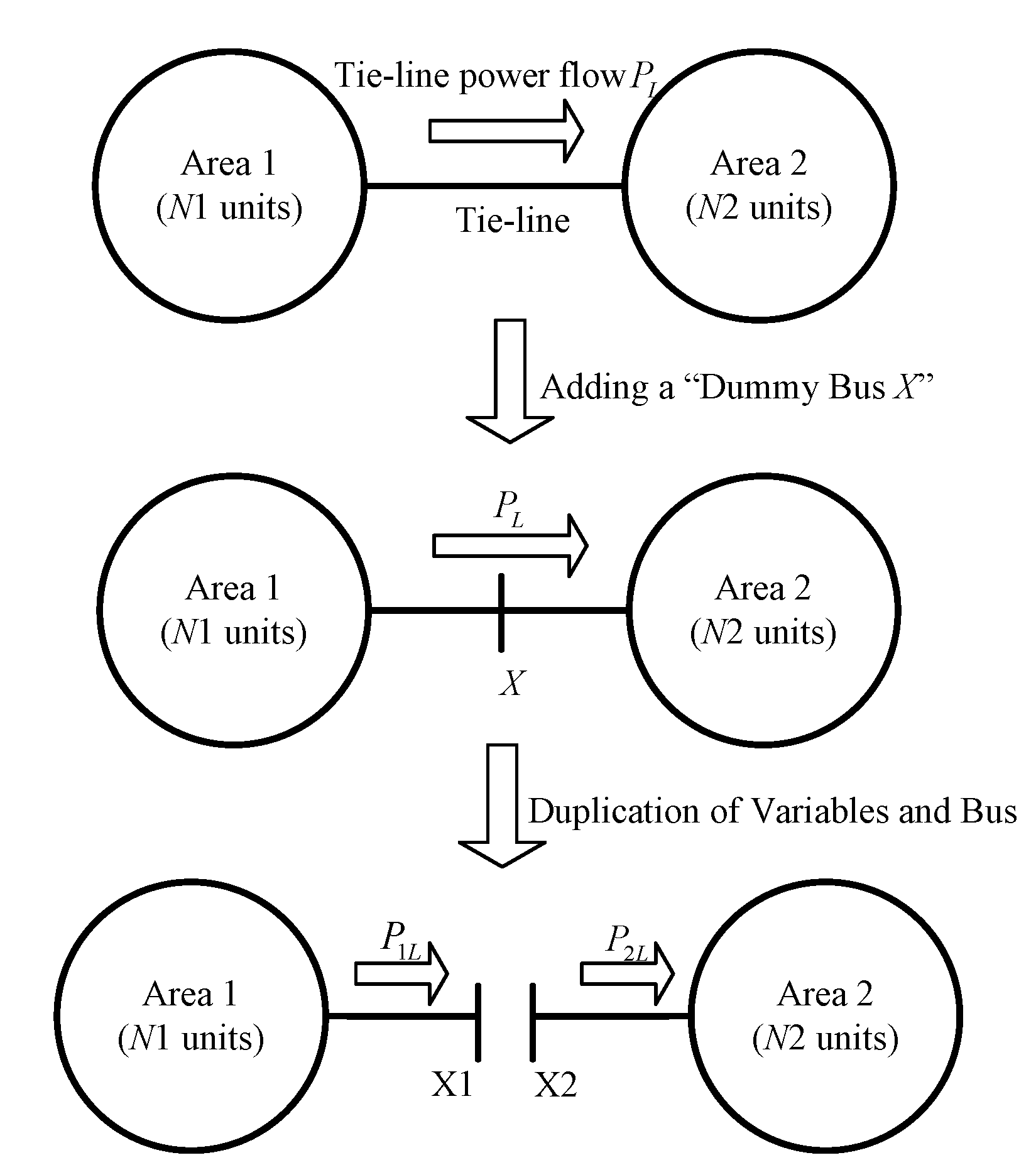
As shown in (7), it is clear that there is a coupling relationship between adjacent areas through the consistency constraint . In this section, with the concept of augmented lagrangian relaxation method and auxiliary problem principle, we will discuss how to divide the original problem (7) into independent sub-problems with the consistency constraint decoupled.
3.1. Augmented Lagrangian Relaxation Method
In this section, we first employ augmented lagrangian relaxation method to deal with the consistency constraint
. Then, the problem (7) can be rewritten as follows.
where
is the Lagrangian multiplier for
;
c>0 is the given penalty factor.
denotes the Euclidean norm of vector
x.
In addition, problem (8) is equivalent to solving a saddle-point problem via the following iterative scheme:
is obtained by solving
then,
is obtained by updating
3.2. Auxiliary Problem Principle
In this section, we take advantage of auxiliary problem principle to cope with the non-separable quadratic term
. The iterative scheme APP for solving problem (8) can be expressed as follows [
14,
15].
Step3. Lagrange multiplier updating
Step4. Check the stop criterion. If
then stop. If not
k=
k+1, go to Step1.
where
β is given APP parameter and
ε denotes step size. The sufficient condition for convergence of APP iterative scheme is given as follow [
13].
Furthermore, experience on applications has illustrated that, for the given penalty parameter
c, the selection of parameters
β and
ε has a significant influence on convergence performance of APP iterative scheme. Ren has pointed that APP iterative scheme can get the best convergence performance when
and
[
16]. Moreover, kim has pointed that convergence performance of APP was reliable with the choice [
13]:
As a result, for the best convergence performance, we choice the APP parameters satisfying in this paper.
4. Auxiliary Problem Principle Method with Self-Adaptive Penalty Parameter
Although, the intrinsic relationship between parameters
β,
ε and
c has been discussion in
section 3.2, how to achieve proper parameters for APP proved to be a challenge. Experience on applications has shown that the convergence results depend on the selection of penalty parameter
c; hence, it is important to estimate a proper penalty parameter. Inspired by Bingsheng He’s modified alternating direction method [
17], we proposed a self-adaptive APP which makes progress in the choice of penalty parameter.
4.1. Motivation
Bingsheng He proposed a modified alternating direction method to deal with problem (8). To be more exact, this method adjusts the penalty parameter
c based on the iterate message [
17].
Now we give the details on how to adjust the penalty parameter
c for better convergence performance. In fact, the solution of problem (8) is equivalent to finding a zero point
e(
wk):
where
is the projection on Ω.
and
denote the gradient of
and
respectively.
Equation (17) offers us an inspiration on how to adjust penalty parameter
c. For the sake of balance, we should adjust the penalty parameter
c such that
, but it is always difficult to achieve. Fortunately, if we use alternating direction method to deal with problem (8), then we will find that [
17]:
Now, we only need to adjust the penalty parameter c such that , it is relatively easy to be achieved. To be more exact, for an iterate , if , we should increase penalty parameter c. By contrast, if , we should decrease penalty parameter c.
4.2. Self-Adaptive Penalty Parameter for Two-Area Economic Dispatch Problem
Inspired by Bingsheng He’s idea, we employ the concept of balance to adjust penalty parameter c during APP’s iteration. However, it is difficult to achieve a balance between , and directly, so we first give Lemma 1 which gives a basic convergence property for APP iterative scheme and is useful for further analysis about how to adjust penalty parameter.
Lemma 1 Let sequence {
wk} is generated by the iterative scheme APP and
w* is the solution of problem (8). Then we have
where
The
M-norm
is denoted by
.
Proof. Solving optimization problem (11) and (12) is equivalent to solving
which satisfies [
18]
and using
, we get
Setting
w=w* in (24), we get,
where
Using the concept of variational inequality [
18], solving optimization problem (8) is equivalent to solving
w* which satisfies
In fact,
F is monotone operator [
19]. We have,
Combing (25) and (28), we get
Using (29), we get,
Based on above discussion, the proof of Lemma 1 is completed.
Furthermore, (20) can be rewritten as follow.
where
It is clear that (31) is Fejér monotone, so we get [
20]
Interestingly, (33) is consistent with APP’s stop criterion, so it is clear that if , then wk+1 can be denoted by w*. Hence, the magnitude of can measure the error between wk and w*.
According to
β=2
c which is described in (16), we get,
Now, for the sake of balance, we only need to adjust penalty parameter c such that .
5. Simulation Results
In this section, we employ two test systems to verify the effectiveness of the proposed self-adaptive APP iterative scheme (SAPP) which is compared with traditional APP iterative scheme. Throughout this paper, stop criterion is set to be , the initial lagrangian multiplier is set to be , the maximum iteration kmax is set to be 100 and the intrinsic relationship between APP’s parameters βij, εij and cij is set to be cij=εij=βij/2.
5.1. Test System 1
This system is composed of four generating units without considering valve-point effect and transmission loss, and all data about generating unit is strict from [
21]. The total load demand for test system 1 is 800MW. In details, all generating units are divided into two areas. Area 1 includes 2 generating units and the corresponding load demand accounts for 70% of the total load demand. Area 2 consists of 2 generating units and makes up 30% of the total load demand. The maximum power flow between area 1 and area 2 is 200 MW.
5.2. Test System 2
This system is constituted of ten generators; valve-point effect and transmission loss are neglected here. The total load demand is set to be 2700 MW. Moreover, test system 2 is divided into three areas as shown in
Fig. 2. Area 1 consists of four generating units; area 2 is comprised of three generating units; area 3 is made up of four generating units. The load demand in area 1 accounts for 50% of the total load demand, the corresponding proportion for area 2 and area 3 are both 25%. The generating unit data with three different fuel options has been taken from [
22]. In this paper, we take the fuel option 1 as the fuel cost. In addition, there are three tie-lines in this system and the limits for tie-lines are all set to be 100MW.
Figure 2.
Test system 2, three-area power system.
Figure 2.
Test system 2, three-area power system.
5.3. Simulation Analysis
Table I and
table II reflect the convergence information of test system 1 and test system 2 respectively. The first column gives initial value of penalty parameter. The second and third columns indicate total number of iterations when the corresponding iterative scheme satisfies stop criterion. The fourth column shows total cost as objective function for MAED problem. Simulation results demonstrate that the APP is sensitive to the selection of initial penalty parameter, if penalty parameter is chosen too big or too small, APP need more number of iteration to reach the optimum. By contrast, the proposed SAPP has better stability in convergence with different penalty parameter, and has better convergence rate.
6. Conclusion
Auxiliary problem principle is one of the attractive approaches to solve multi-area economic dispatch problem and has been applied in many other fields in power systems. However, its convergence performance is significantly influenced by the selection the penalty parameter. In this paper, we propose a self-adaptive APP iterative scheme, which allow the penalty parameter increase or decrease according to iterative information. Simulation results illustrate that the proposed SAPP is superior to the traditional APP in terms of stability in convergence.
Table 1.
Comparison of results for test system 1.
Table 1.
Comparison of results for test system 1.
| Penalty parameter | Number of iterations | Total cost ($/h) |
|---|
| APP | SAPP |
|---|
| 102 | Fail to convergence with maximum iteration 100 | 6 | 7.7549×10³ |
| 101 | Fail to convergence with maximum iteration 100 | 6 |
| 100 | Fail to convergence with maximum iteration 100 | 6 |
| 10-1 | Fail to convergence with maximum iteration 100 | 6 |
| 10-2 | 15 | 7 |
| 10-3 | 45 | 10 |
| 10-4 | Fail to convergence with maximum iteration 100 | 14 |
| 10-5 | Fail to convergence with maximum iteration 100 | 17 |
| 10-6 | Fail to convergence with maximum iteration 100 | 21 |
Table 2.
Comparison of results for test system 2.
Table 2.
Comparison of results for test system 2.
| Penalty parameter | Number of iterations | Total cost ($/h) |
|---|
| APP | SAPP |
|---|
| 102 | Fail to convergence with maximum iteration 100 | 46 | 718.0707 |
| 101 | Fail to convergence with maximum iteration 100 | 31 |
| 100 | Fail to convergence with maximum iteration 100 | 27 |
| 10-1 | Fail to convergence with maximum iteration 100 | 27 |
| 10-2 | Fail to convergence with maximum iteration 100 | 11 |
| 10-3 | 31 | 23 |
| 10-4 | Fail to convergence with maximum iteration 100 | 23 |
| 10-5 | Fail to convergence with maximum iteration 100 | 31 |
| 10-6 | Fail to convergence with maximum iteration 100 | 28 |
Acknowledgments
The authors would like to thank the department of automation of southeast university for providing the necessary facilities and encouragement to carry out this work. This work is supported by State Grid Corporation of China, Major Projects on Planning and Operation Control of Large Scale Grid (SGCC-MPLG022-2012).
Author Contributions
This research was carried out in collaboration among all two authors. Shumin Fei defined the research theme. Yaming Ren designed the algorithm, carried out the experiments and analyzed the data. All authors have read and approved the final manuscript.
Conflicts of Interest
The authors declare no conflict of interest.
References
- Basu, M. Artificial bee colony optimization for multi-area economic dispatch. Int. J. Elec. Power 2013, 49, 181–187. [Google Scholar] [CrossRef]
- Yan, W.; Wen, L.; Li, W.; Chung, C.Y.; Wong, K.P. Decomposition-coordination interior point method and its application to multi-area optimal reactive power flow. Int. J. Elec. Power 2011, 33, 55–60. [Google Scholar] [CrossRef]
- Conejo, A.J.; Nogales, F.J.; Prieto, F.J. A decomposition procedure based on approximate Newton directions. Math. Program 2002, 93, 495–515. [Google Scholar] [CrossRef]
- Nogales, F.J. A decomposition methodology applied to the multi-area optimal power flow problem. Ann. Oper. Res. 2003, 120, 99–116. [Google Scholar] [CrossRef]
- Cohen, G. Auxiliary problem principle and decomposition of optimization problems. J. Optimiz Theory App. 1980, 32, 277–305. [Google Scholar] [CrossRef]
- Batut, J.; Renaud, A. Daily generation scheduling optimization with transmission constraints: a new class of algorithms. IEEE T. Power Syst. 1992, 7, 982–989. [Google Scholar] [CrossRef]
- Beltran, C.; Heredia, F.J. Unit Commitment by Augmented Lagrangian Relaxation: Testing Two Decomposition Approaches. J. Optimiz. Theory App. 2002, 112, 295–314. [Google Scholar] [CrossRef]
- Liu, K.; Li, Y.; Sheng, W. The decomposition and computation method for distributed optimal power flow based on message passing interface (MPI). Int. J. Elec. Power 2011, 33, 1185–1193. [Google Scholar] [CrossRef]
- Chung, K.H.; Kim, B.H.; Hur, D. Distributed implementation of generation scheduling algorithm on interconnected power systems. Energ. Convers. Manage 2011, 52, 3457–3464. [Google Scholar] [CrossRef]
- Somasundaram, P.; Swaroopan, N.M.J. Fuzzified Particle Swarm Optimization Algorithm for Multi-area Security Constrained Economic Dispatch. Elec. Power Compon. Sys. 2011, 39, 979–990. [Google Scholar] [CrossRef]
- Ramesh, V.; Jayabarathi, T.; Asthana, S.; Mital, S.; Basu, S. Combined Hybrid Differential Particle Swarm Optimization Approach for Economic Dispatch Problems. Electr. Power Compon. Sys. 2010, 38, 545–557. [Google Scholar] [CrossRef]
- Fadil, S.; Yazici, A.; Urazel, B. A Security-constrained Economic Power Dispatch Technique Using Modified Subgradient Algorithm Based on Feasible Values and Pseudo Scaling Factor for a Power System Area Including Limited Energy Supply Thermal Units. Electr. Power Compon. Sys. 2011, 39, 1748–1768. [Google Scholar] [CrossRef]
- Kim, B.H.; Baldick, R. Coarse-grained distributed optimal power flow. IEEE T. Power Syst. 1997, 12, 932–939. [Google Scholar] [CrossRef]
- Losi, A. On the application of the auxiliary problem principle. J. Optimiz. Theory App. 2003, 117, 377–396. [Google Scholar] [CrossRef]
- Langenberg, N. Interior point methods for equilibrium problems. Comput. Optim. Appl. 2012, 53, 453–483. [Google Scholar] [CrossRef]
- Ren, Y.; Tian, Y.; Wei, H. Parameter evaluation of auxiliary problem principle for large-scale multi-area economic dispatch. Int. Transactions on Elec. Energ. Sys. 2014, 24, 1782–1790. [Google Scholar] [CrossRef]
- He, B.S.; Yang, H.; Wang, S.L. Alternating direction method with self-adaptive penalty parameters for monotone variational inequalities. J Optimiz. Theory App. 2000, 106, 337–356. [Google Scholar] [CrossRef]
- Yuan, X. An improved proximal alternating direction method for monotone variational inequalities with separable structure. Comput. Optim. Appl. 2011, 49, 17–29. [Google Scholar] [CrossRef]
- He, B.S.; Shen, Y. On the convergence rate of customized proximal point algorithm for convex optimization and saddle-point problem. Sci. Sin. Math. 2012, 42, 515–525. [Google Scholar] [CrossRef]
- He, B.; Yuan, X. Convergence Analysis of Primal-Dual Algorithms for a Saddle-Point Problem: From Contraction Perspective. SIAM J. Imaging Sci. 2012, 5, 119–149. [Google Scholar] [CrossRef]
- Chen, C.L.; Chen, N.M. Direct search method for solving economic dispatch problem considering transmission capacity constraints. IEEE T Power Syst. 2001, 16, 764–769. [Google Scholar] [CrossRef]
- Manoharan, P.S.; Kannan, P.S.; Baskar, S.; Willjuice Iruthayarajan, M. Evolutionary algorithm solution and KKT based optimality verification to multi-area economic dispatch. Int. J. Elec. Power 2009, 31, 365–373. [Google Scholar] [CrossRef]
© 2015 by the authors; licensee MDPI, Basel, Switzerland. This article is an open access article distributed under the terms and conditions of the Creative Commons Attribution license (http://creativecommons.org/licenses/by/4.0/).


