A Clustering Algorithm based on Feature Weighting Fuzzy Compactness and Separation

Abstract

Aiming at improving the well-known fuzzy compactness and separation algorithm (FCS), this paper proposes a new clustering algorithm based on feature weighting fuzzy compactness and separation (WFCS). In view of the contribution of features to clustering, the proposed algorithm introduces the feature weighting into the objective function. We first formulate the membership and feature weighting, and analyze the membership of data points falling on the crisp boundary, then give the adjustment strategy. The proposed WFCS is validated both on simulated dataset and real dataset. The experimental results demonstrate that the proposed WFCS has the characteristics of hard clustering and fuzzy clustering, and outperforms many existing clustering algorithms with respect to three metrics: Rand Index, Xie-Beni Index and Within-Between(WB) Index.

1. Introduction

Similar data belongs to a cluster, while different data belongs to different clusters [1,2,3]. The fuzzy C-means (FCM) algorithm is a classical pattern recognition method [4], and many FCM-type clustering algorithms were proposed [5,6]. However, the between-cluster separation is ignored in these clustering techniques because these algorithms partition data points only by minimizing the distances between data points and cluster centers (i.e., the within-cluster compactness). Therefore, Wu et al. proposed a fuzzy compactness and separation (FCS) algorithm [7]. The proposed FCS algorithm assigns a crisp boundary for each cluster so that hard memberships and fuzzy memberships can co-exist in the clustering results.

For high dimensional dataset clustering, features of data are assigned weights which illustrate the importance degree of features. A major problem of un-weighted clustering algorithms lies in treating all features equally in the clustering process. Therefore, many contributions attempt to weight features with various methods and to optimize the FCM-type algorithms [8,9,10,11,12,13]. Frigui and Nasraoui [8] proposed the simultaneous clustering and attribute discrimination algorithm, in which clustering and feature weighting can be performed simultaneously in an unsupervised manner; Wang et al. [9] discussed that the weight assignment can be given by learning according to the gradient descent technique; Jing et al. proposed an EWkmeans [10] which minimizes the within-cluster compactness and maximizes the negative weight entropy to stimulate more features contributing to the identification of a cluster; Wang et al. [11] presented a new fuzzy C-means algorithm with variable weighting (WFCM) for high dimensional data analysis; Wang et al. [12] put forward a feature weighting fuzzy clustering algorithm integrating rough sets and shadowed sets (WSRFCM); Deng et al. [13] introduced the between-cluster separation into the EWkmeans and proposed the enhanced soft subspace clustering (ESSC) algorithm. The WFCM and WSRFCM employ only the within-cluster compactness while updating the membership matrix and feature weights. ESSC uses a parameter ƞ to balance the within-cluster compactness and between-cluster separation. However, negative values may be produced in the membership matrix if the balancing parameter is too large. Therefore, to avoid the negative membership value, ƞ could be set zero. In this case, ESSC would degrade to the EWkmeans.

In the real world, some data points belong to a cluster strictly (i.e., hard clustering) and others belong to a cluster ambiguously (i.e., fuzzy clustering). For maximizing the between-cluster separation and minimizing the within-cluster compactness, we proposed a new feature weighting fuzzy compactness and separation (WFCS) algorithm with fusion of hard clustering and fuzzy clustering. The rest of this paper is organized as follows. Section 2 introduces both the FCS and the WFCS algorithms, addresses the flaw of FCS and discusses the adjustment of membership and feature weighting of WFCS. The proposed algorithm is evaluated in section 3. Finally, this paper is concluded and the future work is discussed in Section 4.

Table 1 illustrates the main symbols that appear in the following formulas.

2. The FCS and WFCS Algorithms

In this section, the FCS algorithm is reviewed and data points on the crisp boundary are discussed. Then we present the WFCS algorithm, demonstrate the formulas of the membership and feature weight and give the adjustment strategy of these formulas.

$X=\left\{x_1,x_2,...,x_n\right\}$ is a dataset in an s-dimensional Euclidean space ${ℝ}^s$, and $\overline{X}$ denotes the grand mean of $X.$

Table 1. Symbols list.

Symbol	Description
$n$	the numbers of data
$c$	the numbers of clusters
$s$	the numbers of features
$x_j$	the $j\text{th}$ data, $x_j\in {ℝ}^s$
$a_i$	the $i\text{th}$ cluster center, $a_i\in {ℝ}^s$
${\mu }_{ij}$	the membership of the $j\text{th}$ data belonging to the $i\text{th}$ cluster
$m$	the fuzzy exponent
${\omega }_k$	the $k\text{th}$ feature weigh
$\alpha$	the feature weighting exponent
$\eta$	the parameter to control the influence of between-cluster separation

Table 1. Symbols list.

Symbol	Description
$n$	the numbers of data
$c$	the numbers of clusters
$s$	the numbers of features
$x_j$	the $j\text{th}$ data, $x_j\in {ℝ}^s$
$a_i$	the $i\text{th}$ cluster center, $a_i\in {ℝ}^s$
${\mu }_{ij}$	the membership of the $j\text{th}$ data belonging to the $i\text{th}$ cluster
$m$	the fuzzy exponent
${\omega }_k$	the $k\text{th}$ feature weigh
$\alpha$	the feature weighting exponent
$\eta$	the parameter to control the influence of between-cluster separation

2.1. FCS Algorithm [7]

The fuzzy within-cluster compactness $S_{FW}$ and the fuzzy between-cluster separation $S_{FB}$ are defined as:

$$S_{FW}={\displaystyle \sum _{i=1}^c{\displaystyle \sum _{j=1}^n{\mu }_{ij}^m||x_j-a_i{||}^2}}$$

(1)

$$S_{FB}={\displaystyle \sum _{i=1}^c{\displaystyle \sum _{j=1}^n{\mu }_{ij}^m||a_i-\overline{X}{||}^2}}$$

(2)

Objective function is formulated as:

$$\begin{array}{c}{J}_{FCS}=S_{FW}-\eta S_{FB}.{\displaystyle \sum _{i=1}^c{\displaystyle \sum _{j=1}^n{\mu }_{ij}^m||x_j-a_i{||}^2}-}{\displaystyle \sum _{i=1}^c{\eta }_i{\displaystyle \sum _{j=1}^n{\mu }_{ij}^m||a_i-\overline{X}{||}^2}}\\ s.t.{\mu }_{ij}\in \left[0,1\right],{\displaystyle \sum _{i=1}^c{\mu }_{ij}}=1\end{array}$$

(3)

where $\eta =\{{\eta }_1,...,{\eta }_c\}.$

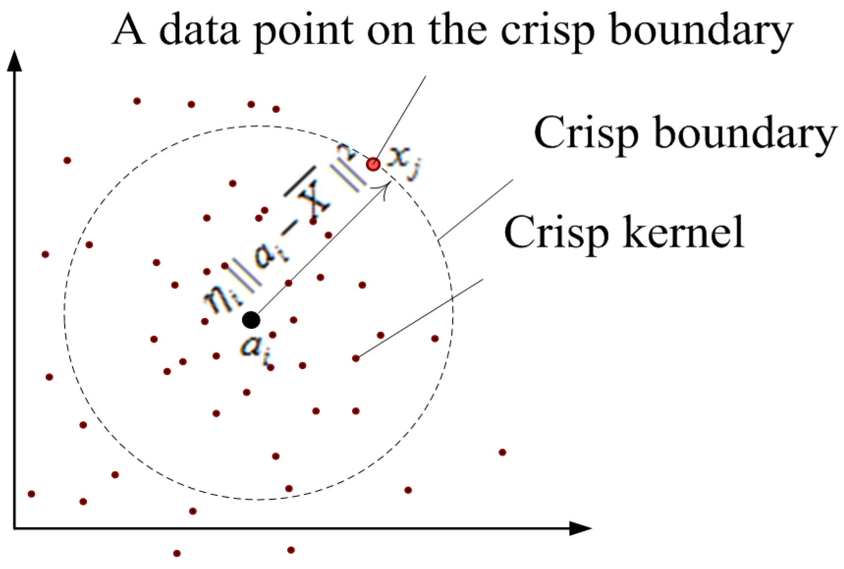
In Equation (3), ${\eta }_i||a_i-\overline{X}{||}^2$ represents the crisp kernel size of $i\text{th}$ cluster (2-dimensional diagram is shown in Figure 1). The parameter ${\eta }_i$ guarantees that no two crisp kernels will overlap [7] and can be demonstrated as:

$${\eta }_i=\frac{\beta }{4}\frac{{\min }_{i\ne i\text{'}}||a_i-a_{i\prime }{||}^2}{{\max }_t||a_t-\overline{X}{||}^2}$$

(4)

where $0\le \beta \le 1$ and $t=1,...,c.$

By minimizing $J_{FCS},$ we have:

$$a_i=\frac{{\displaystyle \sum _{j=1}^n{\mu }_{ij}^m}{x}_j-{\eta }_i{\displaystyle \sum _{j=1}^n{\mu }_{ij}^m}\overline{X}}{{\displaystyle \sum _{j=1}^n{\mu }_{ij}^m}-{\eta }_i{\displaystyle \sum _{j=1}^n{\mu }_{ij}^m}}$$

(5)

$${\mu }_{ij}=\frac{{\left(||x_j-a_i{||}^2-{\eta }_i||a_i-\overline{X}{||}^2\right)}^{\frac{-1}{m-1}}}{{\displaystyle \sum _{t=1}^c{\left(||x_j-a_t{||}^2-{\eta }_t||a_t-\overline{X}{||}^2\right)}^{\frac{-1}{m-1}}}}$$

(6)

According to Equations (5) and (6), dataset $X$ can be partitioned into $c$ clusters by iteratively updating cluster centers and membership value.

The data point in the $i\text{th}$ crisp kernel belongs to the $i\text{th}$ cluster strictly, which is called hard clustering. However, if a data point falls on the crisp boundary (see Figure 1), membership value ${\mu }_{ij}$ will be infinite. Hence, according to Equation (6) the FCS algorithm fails.

Figure 1. Illustration of the crisp kernel.

Figure 1. Illustration of the crisp kernel.

2.2. WFCS Algorithm

2.2.1. The Principle of WFCS

Aiming at clustering data more reasonably, we introduce feature weight into the FCS. Firstly, we define the feature weighting fuzzy within-cluster matrix $S_{WFW}$ and between-cluster matrix $S_{WFB}$ as follows:

$$S_{WFW}={\displaystyle \sum _{i=1}^c{\displaystyle \sum _{j=1}^n{\displaystyle \sum _{k=1}^s{\mu }_{ij}^m{\omega }_k^{\alpha }||x_{jk}-a_{ik}{||}^2}}}$$

(7)

$$S_{WFB}={\displaystyle \sum _{i=1}^c{\displaystyle \sum _{j=1}^n{\displaystyle \sum _{k=1}^s{\eta }_i{\mu }_{ij}^m{\omega }_k^{\alpha }||a_{ik}-\overline{X_k}{||}^2}}}$$

(8)

We extend the formula of ${\eta }_i$ as:

$${\eta }_i=\frac{\beta }{4}\frac{{\min }_{i\ne i\prime }{\omega }^{\alpha }||a_i-a_{i\prime }{||}^2}{{\max }_t{\omega }^{\alpha }||a_t-\overline{X}{||}^2}$$

(9)

Based on Equation (7) and Equation (8), the objective function is shown as:

$$J_{WFCS}={\displaystyle \sum _{i=1}^c{\displaystyle \sum _{j=1}^n{\displaystyle \sum _{k=1}^s{\mu }_{ij}^m{\omega }_k^{\alpha }||x_{jk}-a_{ik}{||}^2}}-}{\displaystyle \sum _{i=1}^c{\displaystyle \sum _{j=1}^n{\displaystyle \sum _{k=1}^s{\eta }_i{\mu }_{ij}^m{\omega }_k^{\alpha }||a_{ik}-\overline{X_k}{||}^2}}}$$

(10)

Hence, WFCS can be formulated as an optimization problem which can be expressed as:

$$\{\begin{array}{cc}\min J_{WFCS}& \\ s.t.{\displaystyle \sum _{i=1}^c{\mu }_{ij}}=1,{\displaystyle \sum _{k=1}^s{\omega }_k}=1& \end{array}$$

(11)

Equation (11) can be solved via the Lagrange multiplier. The L function can be given by:

$$L={\displaystyle \sum _{i=1}^c{\displaystyle \sum _{j=1}^n{\displaystyle \sum _{k=1}^s{\mu }_{ij}^m{\omega }_k^{\alpha }||x_{jk}-a_{ik}{||}^2}}-}{\displaystyle \sum _{i=1}^c{\displaystyle \sum _{j=1}^n{\displaystyle \sum _{k=1}^s{\eta }_i{\mu }_{ij}^m{\omega }_k^{\alpha }||a_{ik}-\overline{X_k}{||}^2}}}+{\displaystyle \sum _{j=1}^n{\lambda }_j\left({\displaystyle \sum _{i=1}^c{\mu }_{ij}}-1\right)}-\gamma \left({\displaystyle \sum _{k=1}^s{\omega }_k}-1\right)$$

(12)

Let the partial derivatives of L function with respect to ${\mu }_{ij}$, ${\omega }_k$, ${\lambda }_j$ and $\gamma$ equal to zero. Then we have:

$$a_{ik}=\frac{{\displaystyle \sum _{j=1}^n{\mu }_{ij}^m}(x_{jk}-{\eta }_i\overline{X_k})}{{\displaystyle \sum _{j=1}^n{\mu }_{ij}^m(1-{\eta }_i)}}$$

(13)

$${\omega }_k=\frac{{\left({\displaystyle \sum _{i=1}^c{\displaystyle \sum _{j=1}^n{\mu }_{ij}^m\left(||x_{jk}-a_{ik}{||}^2-{\eta }_i||a_{ik}-\overline{X_k}{||}^2\right)}}\right)}^{\frac{1}{1-\alpha }}}{{\displaystyle \sum _{t=1}^s{\left({\displaystyle \sum _{i=1}^c{\displaystyle \sum _{j=1}^n{\mu }_{ij}^m\left(||x_{jt}-a_{it}{||}^2-{\eta }_i||a_{it}-\overline{X_t}{||}^2\right)}}\right)}^{\frac{1}{1-\alpha }}}}$$

(14)

$${\mu }_{ij}=\frac{{\left({\displaystyle \sum _{k=1}^s{\omega }_k^{\alpha }\left(||x_{jk}-a_{ik}{||}^2-{\eta }_i||a_{ik}-\overline{X_k}{||}^2\right)}\right)}^{\frac{1}{1-m}}}{{\displaystyle \sum _{t=1}^c{\left({\displaystyle \sum _{k=1}^s{\omega }_k^{\alpha }\left(||x_{jk}-a_{tk}{||}^2-{\eta }_t||a_{tk}-\overline{X_k}{||}^2\right)}\right)}^{\frac{1}{1-m}}}}$$

(15)

According to Equations (13)–(15), dataset $X$ can be partitioned into $c$ clusters by iteratively updating $a$, $\omega$ and $\mu$.

We note here that the objective functions of WFCS and ESSC include the within-cluster compactness and between-cluster separation. However, in ESSC the parameter $\eta$ will be assigned a value at the beginning of the iteration procedure and will be fixed. Furthermore, if $\eta =0,$ the ESSC will degrade to the entropy weighting clustering algorithm without the between-cluster information. However, in the proposed WFCS, $\eta$ will be calculated automatically by the between-cluster information and will not be zero if the parameter $\beta \ne 0$.

2.2.2. The Adjustment Strategies

(1) Adjustment of ${\omega }_k$

Let

$${\text{Δ}}_k={\displaystyle \sum _{i=1}^c{\displaystyle \sum _{j=1}^n{\mu }_{ij}^m\left(||x_{jk}-a_{ik}{||}^2-{\eta }_i||a_{ik}-\overline{X_k}{||}^2\right)}}$$

(16)

then Equation (14) can be written as:

$${\omega }_k=\frac{{{\text{Δ}}_k}^{\frac{1}{1-\alpha }}}{{\displaystyle \sum _{t=1}^s{{\text{Δ}}_k}^{\frac{1}{1-\alpha }}}}$$

(17)

If the value of ${\text{Δ}}_k$ is zero, this means that the $k\text{th}$ feature has exactly the same effect on all clusters then ${\omega }_k$ should be zero.

Here, ${\text{Δ}}_k$ is the grand fuzzy distance between data points and crisp kernels on the $k\text{th}$ feature. Hence, ${\text{Δ}}_k$ is non-negative when distribution of data points is balance and so is ${\omega }_k$. On the contrary, ${\text{Δ}}_k$ is negative when distribution of data points is imbalance and ${\omega }_k$ could be negative. Consequently, we have to make some adjustment. Here, ${\text{Δ}}_p\in \left\{{\text{Δ}}_k|{\text{Δ}}_k\ne 0,k=1,...,s\right\}.$ Therefore, the projection function may be expressed as:

$${\text{Δ}}_p=P\left({\text{Δ}}_p\right)={\text{Δ}}_p-\min \left({\text{Δ}}_t\right)+\underset{{\text{Δ}}_q>0}{\min }\left({\text{Δ}}_q\right)$$

(18)

where $t=1,...,s$ and $p=1,...,s.$

After the adjustment, the feature weighting can be given by Equation (14).

(2) Adjustment of ${\mu }_{ij}$

Let

$${\text{Δ}}_{ij}={\displaystyle \sum _{k=1}^s{\omega }_k^{\alpha }\left(||x_{jk}-a_{ik}{||}^2-{\eta }_i||a_{ik}-\overline{X_k}{||}^2\right)}$$

(19)

then Equation (15) can be presented as:

$${\mu }_{ij}=\frac{{{\text{Δ}}_{ij}}^{\frac{1}{1-m}}}{{\displaystyle \sum _{t=1}^c{{\text{Δ}}_{ij}}^{\frac{1}{1-m}}}}$$

(20)

If $x_j$ falls on the $i\text{th}$ crisp boundary, ${\text{Δ}}_{ij}=0$. Accordingly, the membership value of $x_j$ is infinite. The fact is that the membership value of $x_j$ is fuzzier than that of data point in the crisp kernel. Furthermore, the membership value of $x_j$ is greater than that of data point lying outside crisp kernel. Based on the discussions above, we have the projection function as Equation (21):

$$\text{Δ}=P\left(\text{Δ}\right)=\text{Δ}+\underset{{\text{Δ}}_{tq}>0}{\min }({\text{Δ}}_{tq})$$

(21)

where $\text{Δ}\in \left\{{\text{Δ}}_{ij}|{\text{Δ}}_{ij}\ge 0,i=1,...,c,j=1,...,n\right\},$ $t=1,...,c$ and $q=1,...,n$.

After the adjustment, ${\mu }_{ij}$ can be given by Equation (15).

2.2.3. The Implement of WFCS

Step 1. Choose $\beta ,$ $m,$ $\alpha$ and the iterative error threshold $\epsilon .$ Assign a random membership partition matrix $\left\{{\mu }_{ij}\right\}$ and random values between 0 and 1 to $\eta$. Set the initial iteration counter as $l=1$

Step 2. Update $a_i^{(l)}$ with ${\mu }_{ij}^{(l-1)}$, ${\eta }_i^{(l-1)}$ according to Equation (13);

Step 3. Update ${\omega }_k^{(l)}$ with ${\mu }_{ij}^{(l-1)}$, $a_i^{(l.1)}$, ${\eta }_i^{(l-1)}$ based on both Equations (14) and (18);

Step 4. Update ${\mu }_{ij}^{(l)}$ with ${\omega }_k^{(l.1)}$, $a_i^{(l.1)}$, ${\eta }_i^{(l-1)}$ according to Equations (15) and (21);

Step 5. Compute ${\eta }_i^{(l)}$ with $\beta$, $a_i^{(l)}$ according to Equation (9);

Step 6. Set $l=l+1$ and return to Step 2 until convergence has been reached.

3. Performance Evaluation and Analysis

In this section, the proposed WFCS algorithm has been evaluated by a large number of experiments performed on the simulated dataset and the real dataset. The real datasets include eight UCI benchmarking datasets [14] and a CFM56-type engine dataset (named as ENGINE (ENGINE data can be provided by sending email to the corresponding author)) with measurement noise which has been collected from Air Company. In order to obtain the simulated data, an aero-engine gas path data with Gauss noise (named as LTT) was obtained by a simulation software (developed by the Laboratory of Thermal Turbo machines at the National Technical University of Athens (Downloaded from http://www.ltt.mech.ntua.gr/index.php/softwaremn/teachesmn)). The ENGINE and the LTT datasets present the aero-engine’s states, including healthy states and degrade states. In these experiments, all datasets are normalized into (0, 1) [13].

First, the datasets information, validation criteria and parameters setting are described. Then, the properties of the WFCS are investigated based on the experimental results of the Iris dataset. A detailed comparison with other three feature weighting fuzzy clustering algorithms (ESSC, WFCM, WSRFCM) and one un-weighted fuzzy clustering algorithm (FCS) is performed at last.

3.1. Datasets Information, Validation Criteria and Experimental Setting

The 10 datasets information are summarized in Table 2.

Table 2. Summary of 10 datasets.

Datasets	Size of Dataset	Number of Dimensions	Number of Clusters
Australian	690	14	2
Balance-scale	625	4	3
Breast Cancer	569	30	2
Heart	270	13	2
Iris	150	4	3
Pima	768	8	2
Vehicle	846	18	4
Wine	178	13	3
ENGINE	186	3	2
LTT	300	3	2

Table 2. Summary of 10 datasets.

Datasets	Size of Dataset	Number of Dimensions	Number of Clusters
Australian	690	14	2
Balance-scale	625	4	3
Breast Cancer	569	30	2
Heart	270	13	2
Iris	150	4	3
Pima	768	8	2
Vehicle	846	18	4
Wine	178	13	3
ENGINE	186	3	2
LTT	300	3	2

The rand index (RI) [15], the Xie-Beni index (XB) [16] and Within-Between index (WB) [17] are used for evaluating the performance of the proposed WFCS algorithm. The WB index is a recently proposed one. RI index is defined to evaluate the accuracy of partition—the higher the value is, the higher accuracy we get. XB and WB index are to evaluate the with-cluster compactness and between-cluster separation—the smaller the XB and WB values are, the better the clustering results is.

The parameter setting is: $\alpha <0$ or $\alpha >1$ [18], $m>1,$ $\epsilon ={10}^{‒6}$ and $\beta \in \left\{0.005,0.05,...,1\right\}.$ Parameter values in experiments are tabulated in Table 3, which is based on the best clustering results in terms of the means and standard deviations of the RI index. We conduct each algorithm 10 times. All experiments were implemented on a computer with 2.5 GHz CPU and 8 GB RAM.

Table 3. Parameter values for 10 datasets.

Datasets	WFCS		ESSC		WSRFCM	WFCM	FCS
	β	α	γ	η	α	α	β
Australian	1	−7	1000	0.9	−2	−7	1
Breast Cancer	1	−9	5	0.5	−10	−10	1
Balance-scale	0.01	4	100	0.7	−6	−5	0.05
Heart	0.005	2	100	0	−5	−10	0.5
Iris	1	2	1	0.01	2	2	1
Pima	0.5	−9	100	0.2	−6	−9	1
Vehicle	1	2	50	0.01	4	−10	1
Wine	1	−1	50	0.01	−1	−1	1
ENGINE	1	2	1	0	−10	2	1
LTT	1	−2	1	0	−1	−10	1

Table 3. Parameter values for 10 datasets.

Datasets	WFCS		ESSC		WSRFCM	WFCM	FCS
	β	α	γ	η	α	α	β
Australian	1	−7	1000	0.9	−2	−7	1
Breast Cancer	1	−9	5	0.5	−10	−10	1
Balance-scale	0.01	4	100	0.7	−6	−5	0.05
Heart	0.005	2	100	0	−5	−10	0.5
Iris	1	2	1	0.01	2	2	1
Pima	0.5	−9	100	0.2	−6	−9	1
Vehicle	1	2	50	0.01	4	−10	1
Wine	1	−1	50	0.01	−1	−1	1
ENGINE	1	2	1	0	−10	2	1
LTT	1	−2	1	0	−1	−10	1

3.2. Property Analysis of WFCS

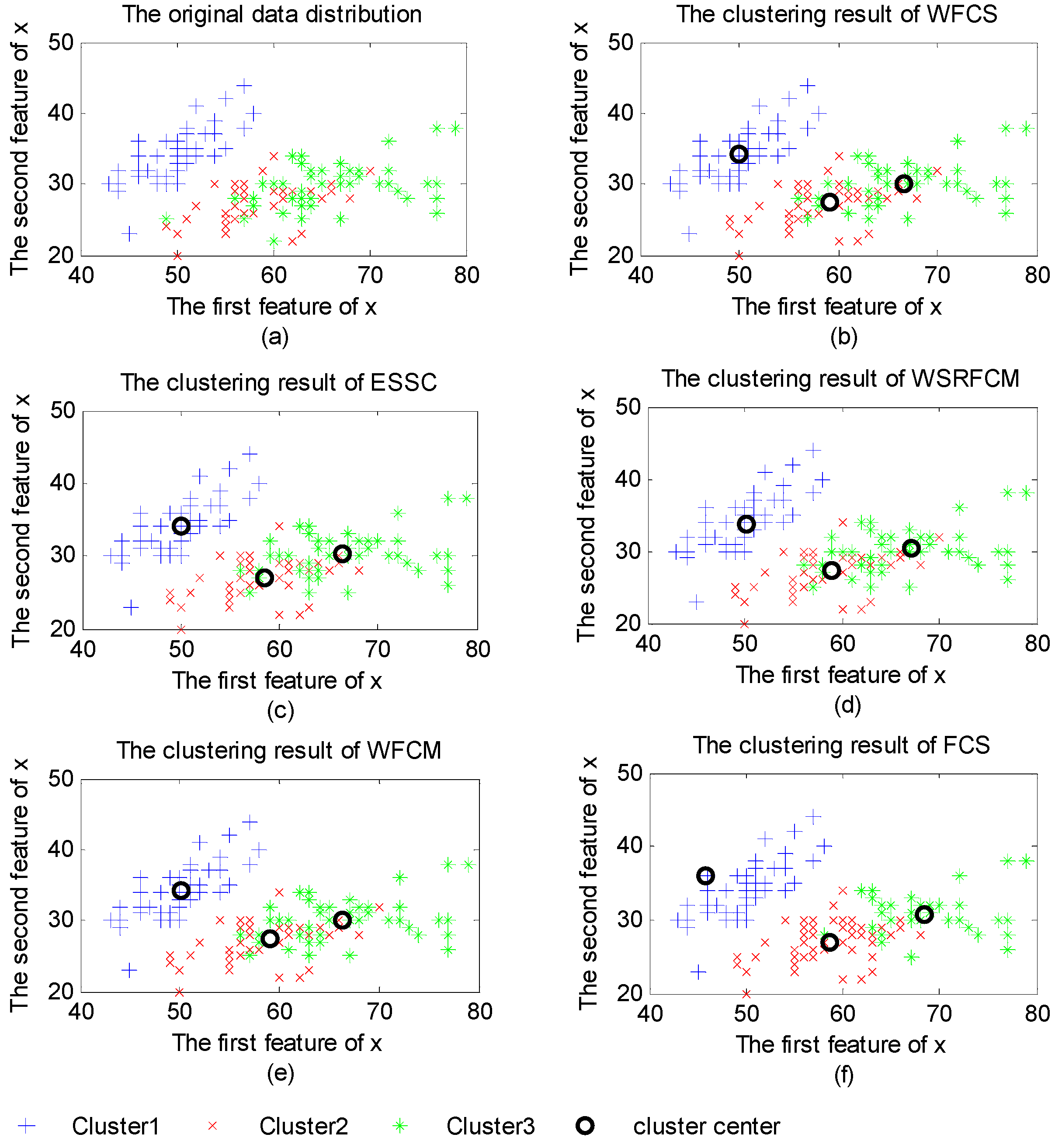
Figure 2 demonstrates the original distribution of Iris dataset and the clustering results of the five algorithms. As shown in Figure 2a, Iris dataset contains three clusters of 50 data points each, where each cluster refers to a type of iris plant. It is obvious that Cluster1 is linearly separable from the other two while the latters are overlapped. Hence, it is more reasonable for data points in Cluster1 to be hard clustered than to be fuzzy clustered.

(1) Clustering performance

Figure 2 shows that clustering results of feature weighted clustering algorithms (WFCS, ESSC, WFCM and WSRFCM) are similar to the distribution of original data (shown in Figure 2 (a)). Data points in Cluster1 can be recognized very well by the five algorithms. Moreover, most data points in Cluster2 and Cluster3 can be recognized by the four feature weighted algorithms. In Figure 2 (f), it is obvious that some data in Cluster3 are misclassified into Cluster2 by FCS.

The cluster centers of five algorithms are different from each other. Furthermore, the distance between Cluster1, Cluster2 and Cluster3 center obtained by the five algorithms are shown in Figure 3.

With regard to WFCS, ESSC and FCS integrating the within-cluster compactness and between-cluster separation, the distances between the overlapped Cluster2 and Cluster3 center are larger than that of WSRFCM and WFCM. However, FCS can’t partition the data points belonging to Cluster2 or Cluster3 correctly for it has not included the feature weight though the biggest value of distance is obtained.

Figure 2. (a) The original data distribution; (b) The clustering results of weighting fuzzy compactness and separation algorithm (WFCS); (c) The clustering results of enhanced soft subspace clustering algorithm (ESSC); (d) The clustering results of the feature weighting fuzzy clustering algorithm integrating rough sets and shadowed sets (WSRFCM); (e) The clustering results of the feature weighting fuzzy c-means algorithm (WFCM); (f) The clustering results of the fuzzy compactness and separation algorithm (FCS).

Figure 2. (a) The original data distribution; (b) The clustering results of weighting fuzzy compactness and separation algorithm (WFCS); (c) The clustering results of enhanced soft subspace clustering algorithm (ESSC); (d) The clustering results of the feature weighting fuzzy clustering algorithm integrating rough sets and shadowed sets (WSRFCM); (e) The clustering results of the feature weighting fuzzy c-means algorithm (WFCM); (f) The clustering results of the fuzzy compactness and separation algorithm (FCS).

Figure 3. The distance between three cluster centers.

Figure 3. The distance between three cluster centers.

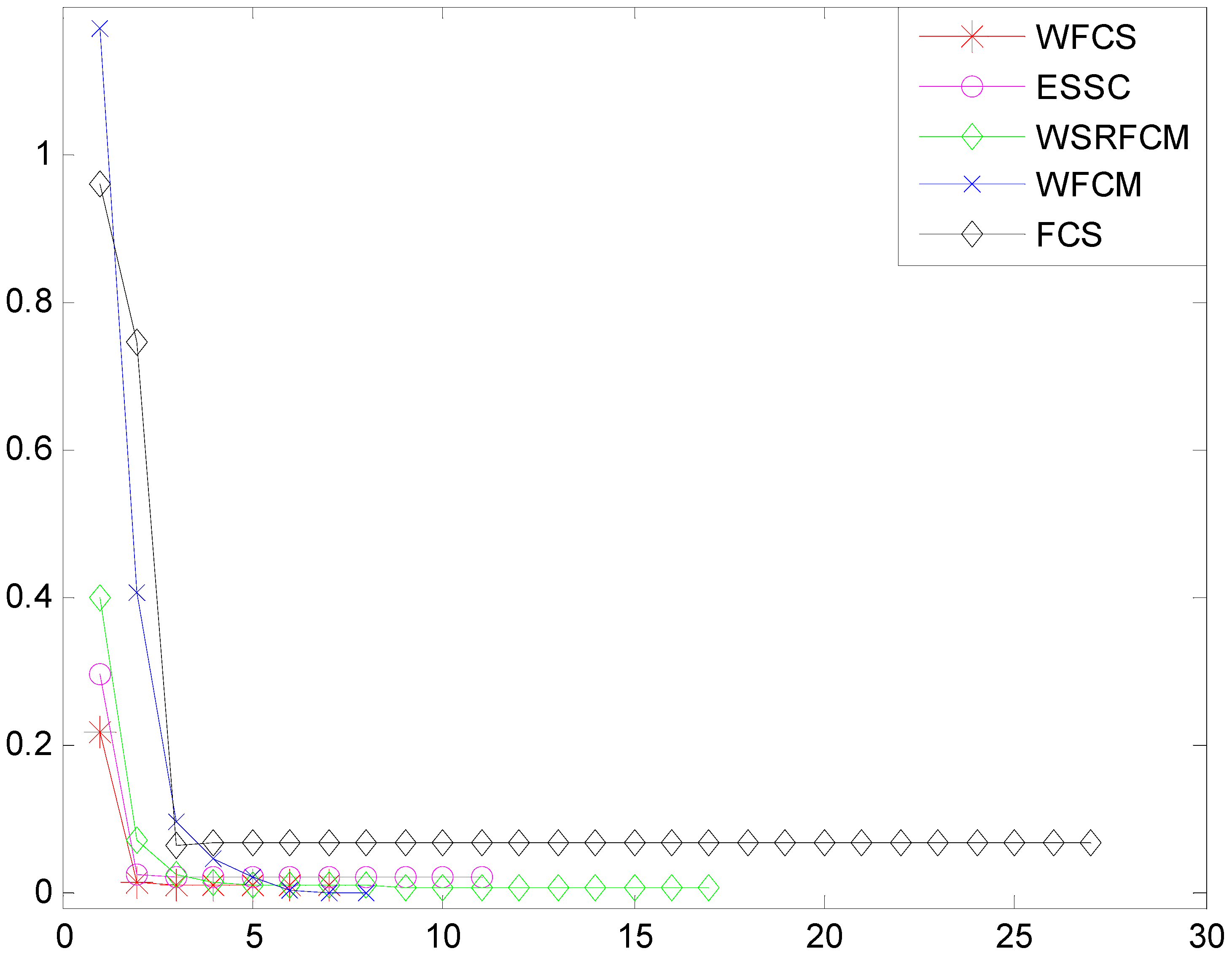
Since different clustering algorithms have different objective functions, we introduce the iteration function $F\left(t\right)=\frac{{\displaystyle \sum _{i=1}^c{\displaystyle \sum _{j=1}^n{\mu }_{ij}||x_j-a_i{||}^2}}}{{\displaystyle \sum _{i=1}^c{\displaystyle \sum _{j=1}^n{\mu }_{ij}||a_i-\overline{X}{||}^2}}}$ in order to evaluate the convergence of algorithm.

Figure 4 shows the convergence curves of the five algorithms.

Figure 4. Convergence of the five algorithms.

Figure 4. Convergence of the five algorithms.

As shown in Figure 4, the five convergence curves descend fast in the first two iterations, and the convergence curves vary slowly after three iterations. Furthermore, the smaller iteration number means the higher convergence speed. Overall, WFCS has a higher speed of convergence. The convergence speed of WFCM is lower than that of WFCS and ESSC, while the FCS has the lowest convergence speed.

(2) Hard clustering

Figure 5 shows the fuzzy membership values for Cluster1 of 150 data points in WFCS when $\beta$ is 1, 0.5, 0.05 and 0.005 respectively. When membership value is equal to 1, data point is hard clustered into Cluster1. When membership value is 0, data point is hard clustered into the other two clusters.

In Figure 5a–c, there are 50, 31 and 12 data points hard clustered into Cluster1 respectively. In Figure 5d, all data point membership values are smaller than 1, then all data points are fuzzy clustered into Cluster1. As seen in Figure 5, the membership value becomes fuzzier when $\beta$ is smaller. Hence, WFCS has the characteristics of both hard clustering and fuzzy clustering.

3.3. Clustering Evaluation

The best RI indexes of the five algorithms are presented in Table 4.

Figure 5. Fuzzy membership value on the first cluster with different $\beta$ (a) $\beta =1$; (b) $\beta =0.5$; (c) $\beta =0.05$; (d) $\beta =0.005$.

Figure 5. Fuzzy membership value on the first cluster with different $\beta$ (a) $\beta =1$; (b) $\beta =0.5$; (c) $\beta =0.05$; (d) $\beta =0.005$.

It is evident in Table 4 that WFCS demonstrates the best performance except for Breast-cancer, Vehicle and ENGINE datasets. The performance of WFCM and WSRFCM are mostly comparable or better than that of ESSC and FCS. Even if FCS is not a feature weighted clustering algorithm, it is able to achieve the best clustering result performance for the dataset Wine. Table 5 and Table 6 list the XB and WB index values of the five algorithms respectively. By comparing Table 4, Table 5 and Table 6, we found that the best clustering performance as indicated through RI is not always the smallest value as indicated through XB or WB index. Therefore, no single algorithm can always be superior to the others for all datasets.

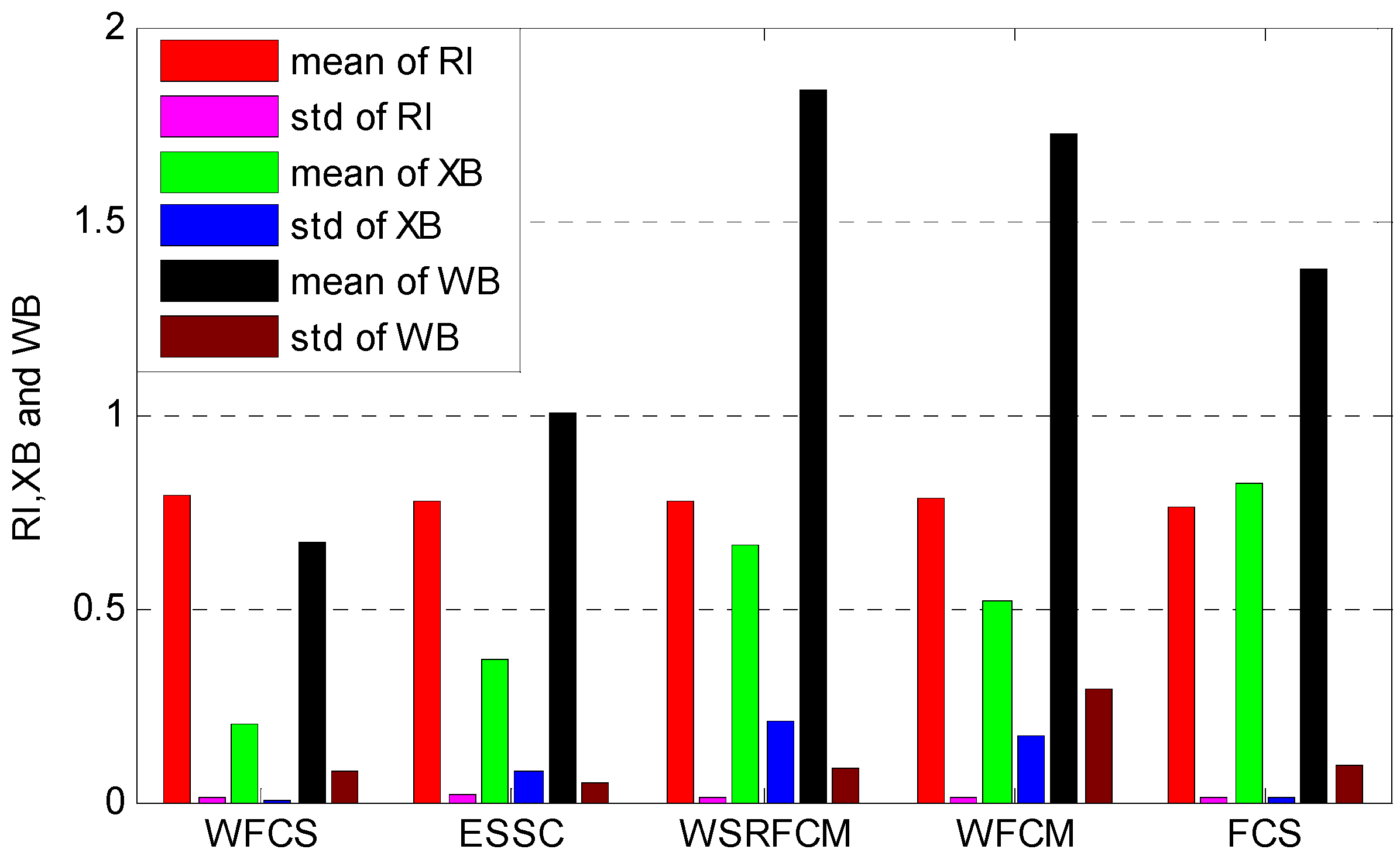
The average performances of the five algorithms are shown in Figure 6.

Figure 6. The average performances of the five algorithms.

Figure 6. The average performances of the five algorithms.

Table 4. The best clustering results obtained for the 10 datasets with rand index (RI).

Dataset	WFCS	ESSC	WSRFCM	WFCM	FCS
Australian
mean	0.7336	0.7162	0.7302	0.7265	0.6995
std	0.0000	0.1134	0.0033	0.0569	0.0125
Breast Cancer
mean	0.8721	0.8779	0.8630	0.8600	0.8627
std	0.0009	0.0057	0	0.0000	0.0000
Balance-scale
mean	0.6427	0.6389	0.6101	0.6099	0.6201
std	0.0758	0.0287	0.0586	0.0578	0.0662
Heart
mean	0.7163	0.7114	0.7120	0.6939	0.6833
std	0.0000	0.0019	0.0023	0.0000	0.0000
Iris
mean	0.9495	0.9195	0.9495	0.9495	0.8679
std	0.0000	0.0000	0.0081	0.0000	0.0000
Pima
mean	0.5841	0.5564	0.5698	0.5837	0.5576
std	0.0000	0.0005	0.0044	0.0009	0.0000
Vehicle
mean	0.6654	0.6539	0.6778	0.6581	0.6528
std	0.0025	0.0028	0.0006	0.0038	0.0000
Wine
mean	0.9551	0.9398	0.9324	0.9398	0.9551
std	0.0000	0.0095	0.0000	0.0000	0.0000
ENGINE
mean	0.8600	0.7823	0.7693	0.8600	0.7903
std	0.0000	0.0005	0.0067	0.0000	0.0000
LTT
mean	0.9671	0.96	0.9543	0.9671	0.9607
std	0.0000	0.0000	0.0000	0.0000	0.0000

Table 4. The best clustering results obtained for the 10 datasets with rand index (RI).

Dataset	WFCS	ESSC	WSRFCM	WFCM	FCS
Australian
mean	0.7336	0.7162	0.7302	0.7265	0.6995
std	0.0000	0.1134	0.0033	0.0569	0.0125
Breast Cancer
mean	0.8721	0.8779	0.8630	0.8600	0.8627
std	0.0009	0.0057	0	0.0000	0.0000
Balance-scale
mean	0.6427	0.6389	0.6101	0.6099	0.6201
std	0.0758	0.0287	0.0586	0.0578	0.0662
Heart
mean	0.7163	0.7114	0.7120	0.6939	0.6833
std	0.0000	0.0019	0.0023	0.0000	0.0000
Iris
mean	0.9495	0.9195	0.9495	0.9495	0.8679
std	0.0000	0.0000	0.0081	0.0000	0.0000
Pima
mean	0.5841	0.5564	0.5698	0.5837	0.5576
std	0.0000	0.0005	0.0044	0.0009	0.0000
Vehicle
mean	0.6654	0.6539	0.6778	0.6581	0.6528
std	0.0025	0.0028	0.0006	0.0038	0.0000
Wine
mean	0.9551	0.9398	0.9324	0.9398	0.9551
std	0.0000	0.0095	0.0000	0.0000	0.0000
ENGINE
mean	0.8600	0.7823	0.7693	0.8600	0.7903
std	0.0000	0.0005	0.0067	0.0000	0.0000
LTT
mean	0.9671	0.96	0.9543	0.9671	0.9607
std	0.0000	0.0000	0.0000	0.0000	0.0000

Table 5. Xie-Beni (XB) index of algorithms.

Dataset	WFCS	ESSC	WSRFCM	WFCM	FCS
Australian
mean	0.0400	0.7194	1.4636	1.2056	0.1995
std	0.0007	0.3455	0.8407	1.0488	0.0267
Breast Cancer
mean	0.3216	0.2961	0.4288	0.3270	0.1094
std	0.0021	0.0344	0.0903	0.0003	0.0000
Balance-scale
mean	0.4435	0.7051	0.6970	0.7392	2.8475
std	0.0000	0.0248	0.0287	0.0725	0.0979
Heart
mean	0.1593	0.4033	0.7942	0.6348	0.2267
std	0.0081	0.0982	0.7522	0.5030	0.0000
Iris
mean	0.0844	0.0861	0.2700	0.1964	0.2922
std	0.0019	0.0059	0.0226	0.0000	0.0000
Pima
mean	0.1443	0.4942	0.7610	0.5955	0.4759
std	0.0002	0.0235	0.1977	0.0406	0.0000
Vehicle
mean	0.2532	0.2601	0.8538	0.5480	3.2949
std	0.0000	0.0917	0.0372	0.0047	0.0097
Wine
mean	0.2577	0.3970	0.6775	0.4987	0.4061
std	0.0034	0.0009	0.0640	0.0000	0.0000
ENGINE
mean	0.1699	0.1836	0.3755	0.2130	0.1267
std	0.0030	0.0685	0.0295	0.0217	0.0000
LTT
mean	0.1019	0.1075	0.3299	0.2131	0.2105
std	0.0014	0.0983	0.0029	0.0000	0.0000

Table 5. Xie-Beni (XB) index of algorithms.

Dataset	WFCS	ESSC	WSRFCM	WFCM	FCS
Australian
mean	0.0400	0.7194	1.4636	1.2056	0.1995
std	0.0007	0.3455	0.8407	1.0488	0.0267
Breast Cancer
mean	0.3216	0.2961	0.4288	0.3270	0.1094
std	0.0021	0.0344	0.0903	0.0003	0.0000
Balance-scale
mean	0.4435	0.7051	0.6970	0.7392	2.8475
std	0.0000	0.0248	0.0287	0.0725	0.0979
Heart
mean	0.1593	0.4033	0.7942	0.6348	0.2267
std	0.0081	0.0982	0.7522	0.5030	0.0000
Iris
mean	0.0844	0.0861	0.2700	0.1964	0.2922
std	0.0019	0.0059	0.0226	0.0000	0.0000
Pima
mean	0.1443	0.4942	0.7610	0.5955	0.4759
std	0.0002	0.0235	0.1977	0.0406	0.0000
Vehicle
mean	0.2532	0.2601	0.8538	0.5480	3.2949
std	0.0000	0.0917	0.0372	0.0047	0.0097
Wine
mean	0.2577	0.3970	0.6775	0.4987	0.4061
std	0.0034	0.0009	0.0640	0.0000	0.0000
ENGINE
mean	0.1699	0.1836	0.3755	0.2130	0.1267
std	0.0030	0.0685	0.0295	0.0217	0.0000
LTT
mean	0.1019	0.1075	0.3299	0.2131	0.2105
std	0.0014	0.0983	0.0029	0.0000	0.0000

In Figure 6, we can see that WFCS obtained the best mean values of RI (0.7946) and XB (0.1976) with the least standard variation (0.0079, 0.0021 respectively) for the 10 datasets. WFCM, WSRFCM and ESSC perform similarly in terms of RI. It can be seen that the feature weighting clustering algorithms are superior to the un-weighted clustering one. The average XB and WB index values of WFCS, ESSC and FCS are smaller than those of WFCM and WSRFCM, which demonstrate that these three algorithms integrating between-cluster separation and within-cluster compactness can partition data points more reasonably.

Table 6. Within-Between(WB) index of algorithms.

Dataset	WFCS	ESSC	WSRFCM	WFCM	FCS
Australian
mean	0.0551	0.1730	0.6312	0.7261	0.5971
std	0.0000	0.1313	0.0011	0.4054	0.2144
Breast Cancer
mean	0.3849	0.3843	0.5388	0.6035	0.4510
std	0.0010	0.0084	0.0000	0.0000	0.0000
Balance-scale
mean	2.1924	3.6567	5.8354	6.1232	5.6191
std	0.7932	0.1983	0.0911	0.1686	0.7135
Heart
mean	1.1191	1.1191	2.3297	3.3005	1.8087
std	0.0000	0.0991	0.0012	0.0000	0.0000
Iris
mean	0.0729	0.3300	0.8423	0.6224	0.5366
std	0.0079	0.0097	0.6452	0.0311	0.0000
Pima
mean	0.2828	0.6195	1.0043	0.4897	0.4832
std	0.0012	0.0003	0.0627	0.0073	0.0000
Vehicle
mean	0.1908	0.2850	0.5000	0.4128	0.6351
std	0.0010	0.0087	0.0149	0.0000	0.0000
Wine
mean	0.9821	0.9934	2.0174	1.4317	0.8599
std	0.0038	0.0350	0.0028	0.0000	0.0000
ENGINE
mean	0.4866	0.8500	1.6315	1.6072	0.8484
std	0.0079	0.0060	0.0056	2.3408	0.0000
LTT
mean	0.9206	1.6253	3.0179	1.9023	1.8894
std	0.0075	0.0281	0.0106	0.0002	0.0000

Table 6. Within-Between(WB) index of algorithms.

Dataset	WFCS	ESSC	WSRFCM	WFCM	FCS
Australian
mean	0.0551	0.1730	0.6312	0.7261	0.5971
std	0.0000	0.1313	0.0011	0.4054	0.2144
Breast Cancer
mean	0.3849	0.3843	0.5388	0.6035	0.4510
std	0.0010	0.0084	0.0000	0.0000	0.0000
Balance-scale
mean	2.1924	3.6567	5.8354	6.1232	5.6191
std	0.7932	0.1983	0.0911	0.1686	0.7135
Heart
mean	1.1191	1.1191	2.3297	3.3005	1.8087
std	0.0000	0.0991	0.0012	0.0000	0.0000
Iris
mean	0.0729	0.3300	0.8423	0.6224	0.5366
std	0.0079	0.0097	0.6452	0.0311	0.0000
Pima
mean	0.2828	0.6195	1.0043	0.4897	0.4832
std	0.0012	0.0003	0.0627	0.0073	0.0000
Vehicle
mean	0.1908	0.2850	0.5000	0.4128	0.6351
std	0.0010	0.0087	0.0149	0.0000	0.0000
Wine
mean	0.9821	0.9934	2.0174	1.4317	0.8599
std	0.0038	0.0350	0.0028	0.0000	0.0000
ENGINE
mean	0.4866	0.8500	1.6315	1.6072	0.8484
std	0.0079	0.0060	0.0056	2.3408	0.0000
LTT
mean	0.9206	1.6253	3.0179	1.9023	1.8894
std	0.0075	0.0281	0.0106	0.0002	0.0000

4. Conclusions

In this paper, a fuzzy clustering algorithm is proposed based on FCS by maximizing the between-cluster matrix and minimizing the within-cluster matrix with weighted features. Two adjustment formulations are derived for adjusting the values of ${\mu }_{ij}$ and the ${\omega }_k$ respectively. Through the proposed WFCS, problem for the membership of the data point lying on the crisp boundary can be solved. Experimental results show that the proposed WFCS generally outperforms the four existing clustering algorithms (FCS, WFCM, WSRFCM and ESSC).

The proposed algorithm can handle linear datasets, whereas, the high-dimensional nonlinear data has not been considered in this paper. In the future, we will employ the kernel methodology [19,20,21] to analyze the high-dimensional nonlinear data.

References

1. Hartigan, J. Clustering Algorithms; Wiley: New York, NY, USA, 1975. [Google Scholar]
2. Jain, A.K.; Murty, M.N.; Flynn, P.J. Data clustering: A review. ACM Comput. Surv. (CSUR) 1999, 31, 264–323. [Google Scholar] [CrossRef]
3. Xu, R.; Wunsch, D. Survey of clustering algorithms. Neu. Net. IEEE Transactions on 2005, 16, 645–678. [Google Scholar] [CrossRef]
4. Bezdek, J.C. Pattern Recognition with Fuzzy Objective Function Algorithms; Plenum Press: New York, NY, USA, 1981. [Google Scholar]
5. Wei, L.M.; Xie, W.X. Rival checked fuzzy c-means algorithm. Acta Electron. Sinica 2000, 28, 63–66. [Google Scholar]
6. Fan, J.L.; Zhen, W.Z.; Xie, W.X. Suppressed fuzzy c-means clustering algorithm. Pattern Recognit. Lett. 2003, 24, 1607–1612. [Google Scholar] [CrossRef]
7. Wu, K.L.; Yu, J.; Yang, M.S. A novel fuzzy clustering algorithm based on a fuzzy scatter matrix with optimality tests. Pattern Recognit. Lett. 2005, 26, 639–652. [Google Scholar] [CrossRef]
8. Frigui, H.; Nasraoui, O. Unsupervised learning of prototypes and feature weights. Pattern Recognit. 2004, 37, 567–581. [Google Scholar] [CrossRef]
9. Wang, X.; Wang, Y.; Wang, L. Improving fuzzy c-means clustering based on feature-weight learning. Pattern Recognit. Lett. 2004, 25, 1123–1132. [Google Scholar] [CrossRef]
10. Jing, L.; Ng, M.K.; Huang, J.Z. An entropy weighting k-means algorithm for subspace clustering of high-dimensional sparse data. Knowl. Data Engin. IEEE Transactions on 2007, 19, 1026–1041. [Google Scholar] [CrossRef]
11. Wang, Q.; Ye, Y.; Huang, J.Z. Fuzzy k-means with variable weighting in high dimensional data analysis. In Proceedings of Web-Age Information Management, 2008, WAIM'08. The Ninth International Conference on. Hunan, China; 2008; pp. 365–372. [Google Scholar]
12. Wang, L.; Wang, J. Feature weighting fuzzy clustering integrating rough sets and shadowed sets. Int. J. Pattern Recognit. Artif. Intell. 2012, 26, 1769–1776. [Google Scholar]
13. Deng, Z.; Choi, K.S.; Chung, F.L.; Wang, S.T. Enhanced soft subspace clustering integrating within-cluster and between-cluster information. Pattern Recognit. 2010, 43, 767–781. [Google Scholar] [CrossRef]
14. Lichman, M. UCI Machine Learning Repository; University of California: Irvine, CA, USA, 2013. [Google Scholar]
15. Rand, W.M. Objective criteria for the evaluation of clustering methods. J. Am. Stat. Assoc. 1971, 66, 846–850. [Google Scholar] [CrossRef]
16. Xie, X.L.; Beni, G.A. A validity measure for fuzzy clustering. IEEE Trans. Pattern Anal. Mach. Intell. 1991, 13, 841–847. [Google Scholar] [CrossRef]
17. Zhao, Q.; Fränti, P. WB-index: A sum-of-squares based index for cluster validity. Data Knowl. Eng. 2014, 92, 77–89. [Google Scholar] [CrossRef]
18. Huang, J.Z; Ng, M.K; Rong, H.; Li, Z.C. Automated variable weighting in k-means type clustering. IEEE Trans. Pattern Anal. Mach. Intell. 2005, 27, 657–668. [Google Scholar] [CrossRef] [PubMed]
19. Filippone, M.; Camastra, F.; Masulli, F.; Rovetta, S. A survey of kernel and spectral methods for clustering. Pattern Recognit. 2008, 41, 176–190. [Google Scholar] [CrossRef]
20. Huang, H.C.; Chuang, Y.Y.; Chen, C.S. Multiple kernel fuzzy clustering. Fuzzy Syst. IEEE Transactions on 2012, 20, 120–134. [Google Scholar] [CrossRef]
21. Lin, K.P. A Novel Evolutionary Kernel Intuitionistic Fuzzy C-means Clustering Algorithm. Fuzzy Syst. IEEE Transactions on 2014, 22, 1074–1087. [Google Scholar] [CrossRef]