
A Clustering Algorithm based on Feature Weighting Fuzzy Compactness and Separation


Abstract
:1. Introduction
2. The FCS and WFCS Algorithms

| Symbol | Description |
|---|---|
| the numbers of data | |
| the numbers of clusters | |
| the numbers of features | |
| the data, | |
| the cluster center, | |
| the membership of the data belonging to the cluster | |
| the fuzzy exponent | |
| the feature weigh | |
| the feature weighting exponent | |
| the parameter to control the influence of between-cluster separation |
2.1. FCS Algorithm [7]
2.2. WFCS Algorithm
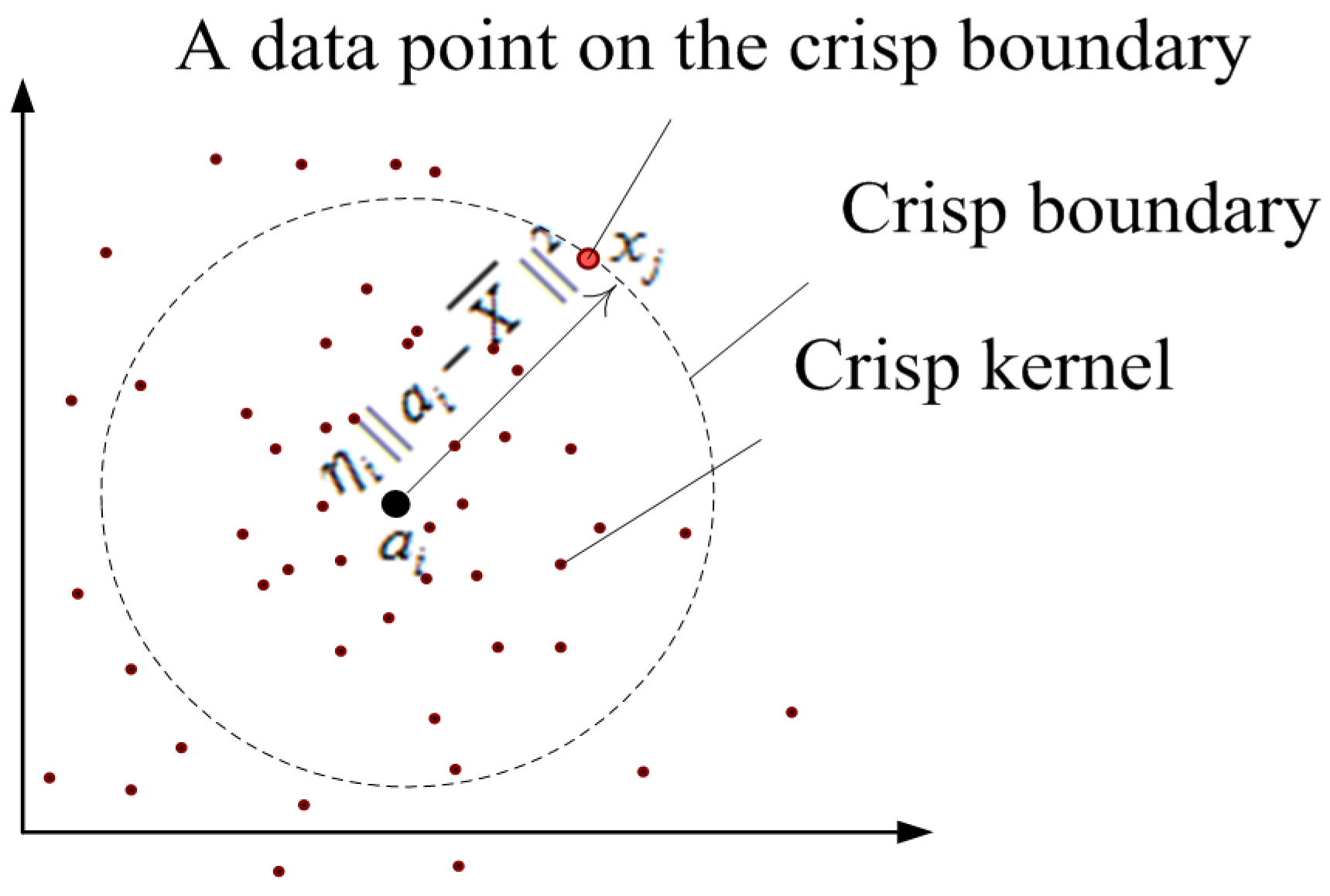
2.2.1. The Principle of WFCS
2.2.2. The Adjustment Strategies
2.2.3. The Implement of WFCS
3. Performance Evaluation and Analysis
3.1. Datasets Information, Validation Criteria and Experimental Setting
| Datasets | Size of Dataset | Number of Dimensions | Number of Clusters |
|---|---|---|---|
| Australian | 690 | 14 | 2 |
| Balance-scale | 625 | 4 | 3 |
| Breast Cancer | 569 | 30 | 2 |
| Heart | 270 | 13 | 2 |
| Iris | 150 | 4 | 3 |
| Pima | 768 | 8 | 2 |
| Vehicle | 846 | 18 | 4 |
| Wine | 178 | 13 | 3 |
| ENGINE | 186 | 3 | 2 |
| LTT | 300 | 3 | 2 |
| Datasets | WFCS | ESSC | WSRFCM | WFCM | FCS | ||
|---|---|---|---|---|---|---|---|
| β | α | γ | η | α | α | β | |
| Australian | 1 | −7 | 1000 | 0.9 | −2 | −7 | 1 |
| Breast Cancer | 1 | −9 | 5 | 0.5 | −10 | −10 | 1 |
| Balance-scale | 0.01 | 4 | 100 | 0.7 | −6 | −5 | 0.05 |
| Heart | 0.005 | 2 | 100 | 0 | −5 | −10 | 0.5 |
| Iris | 1 | 2 | 1 | 0.01 | 2 | 2 | 1 |
| Pima | 0.5 | −9 | 100 | 0.2 | −6 | −9 | 1 |
| Vehicle | 1 | 2 | 50 | 0.01 | 4 | −10 | 1 |
| Wine | 1 | −1 | 50 | 0.01 | −1 | −1 | 1 |
| ENGINE | 1 | 2 | 1 | 0 | −10 | 2 | 1 |
| LTT | 1 | −2 | 1 | 0 | −1 | −10 | 1 |
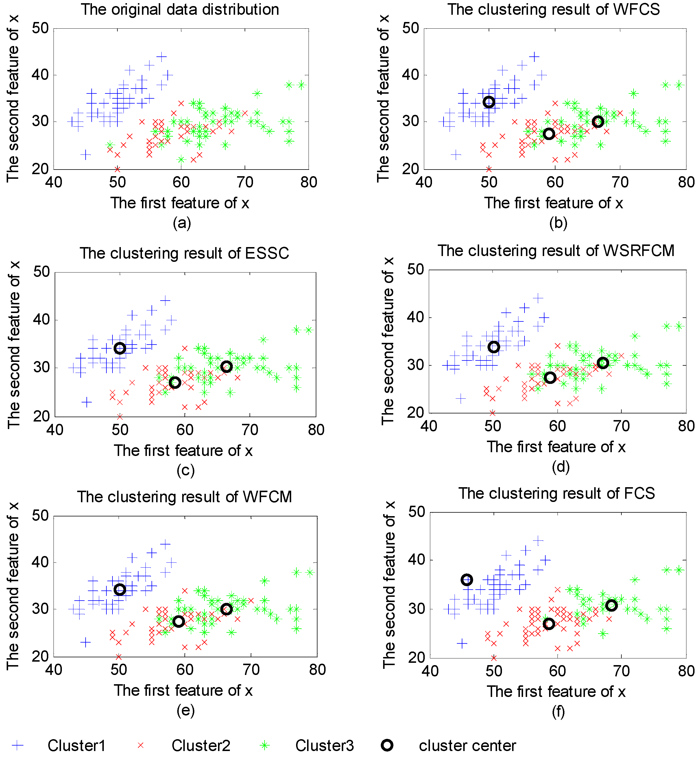
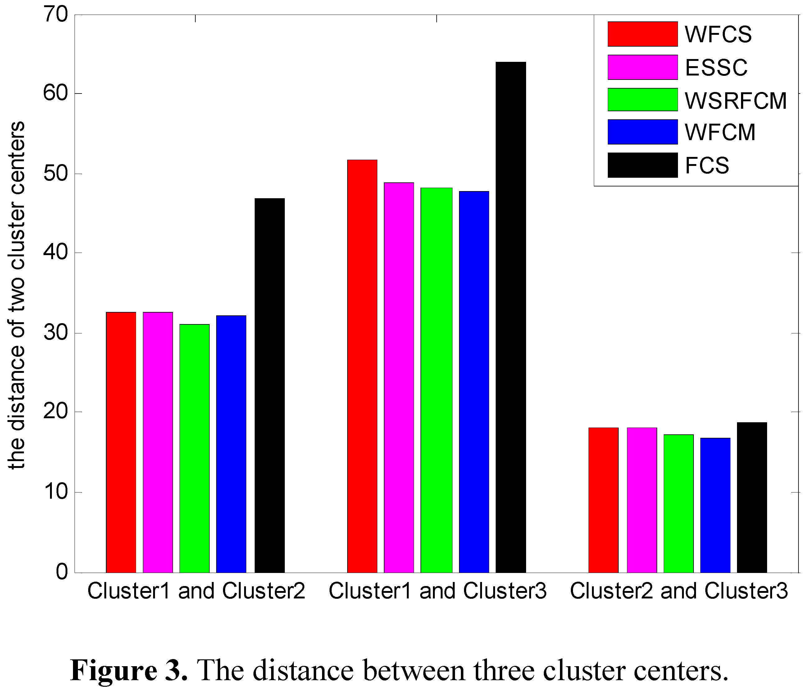
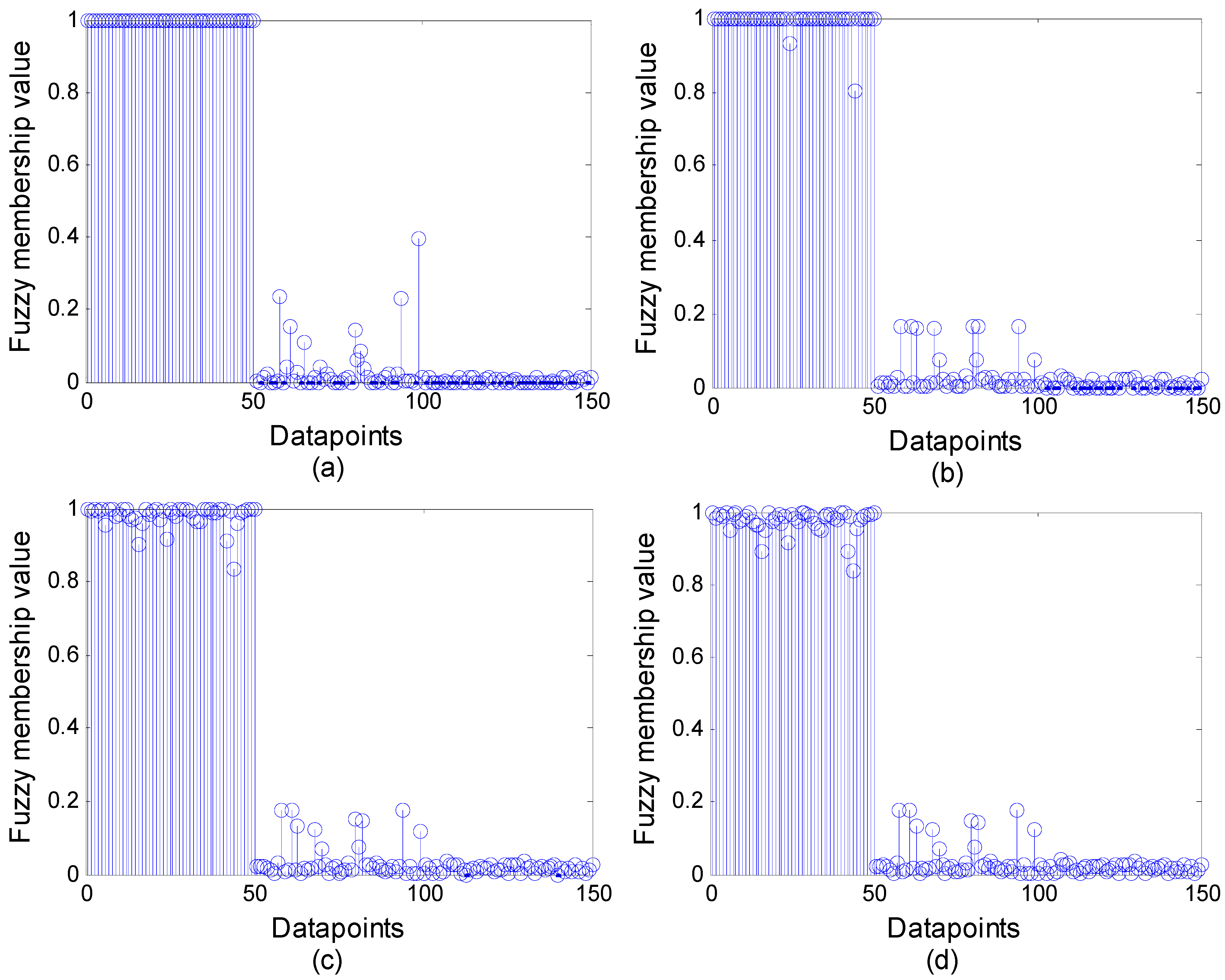
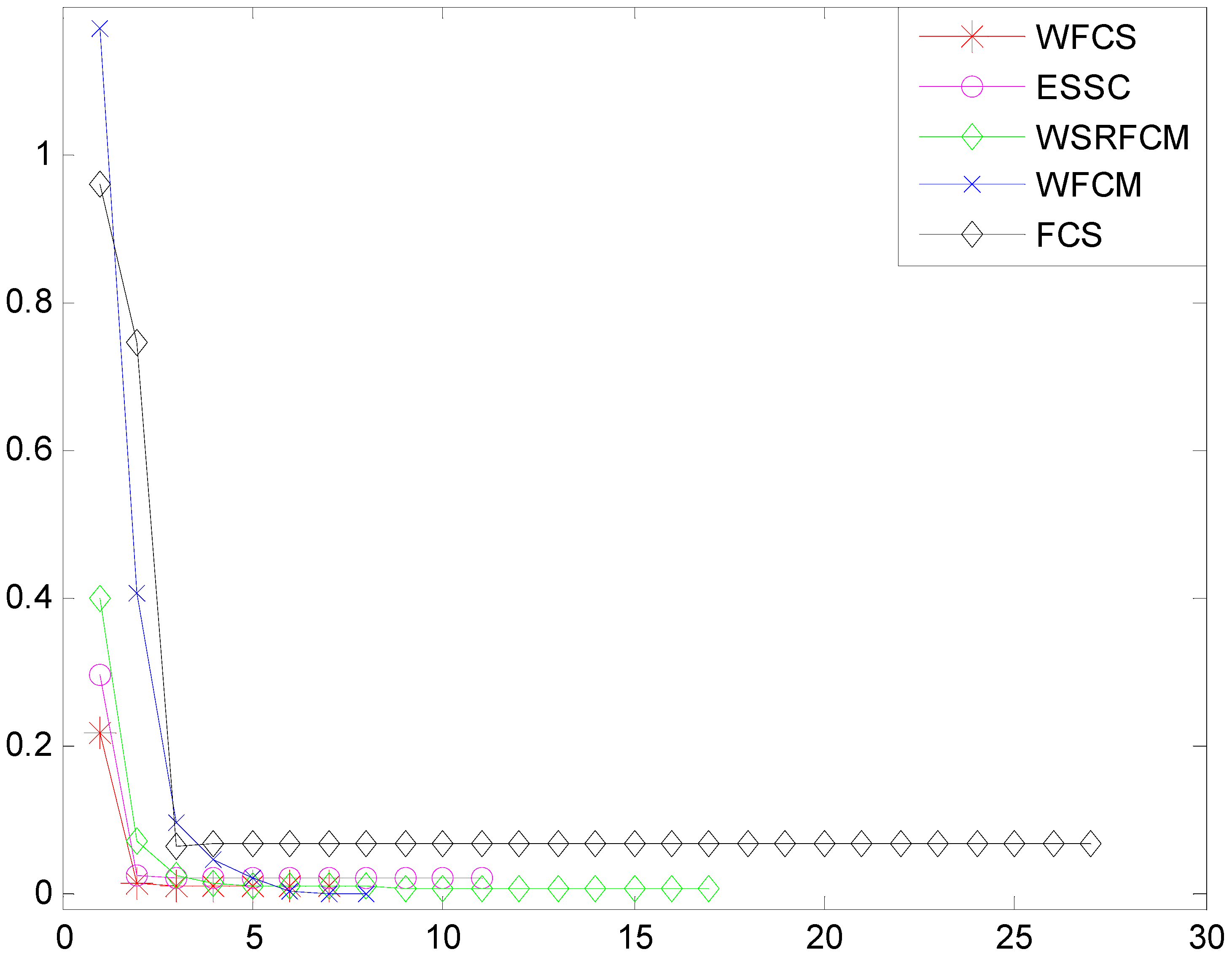
3.2. Property Analysis of WFCS


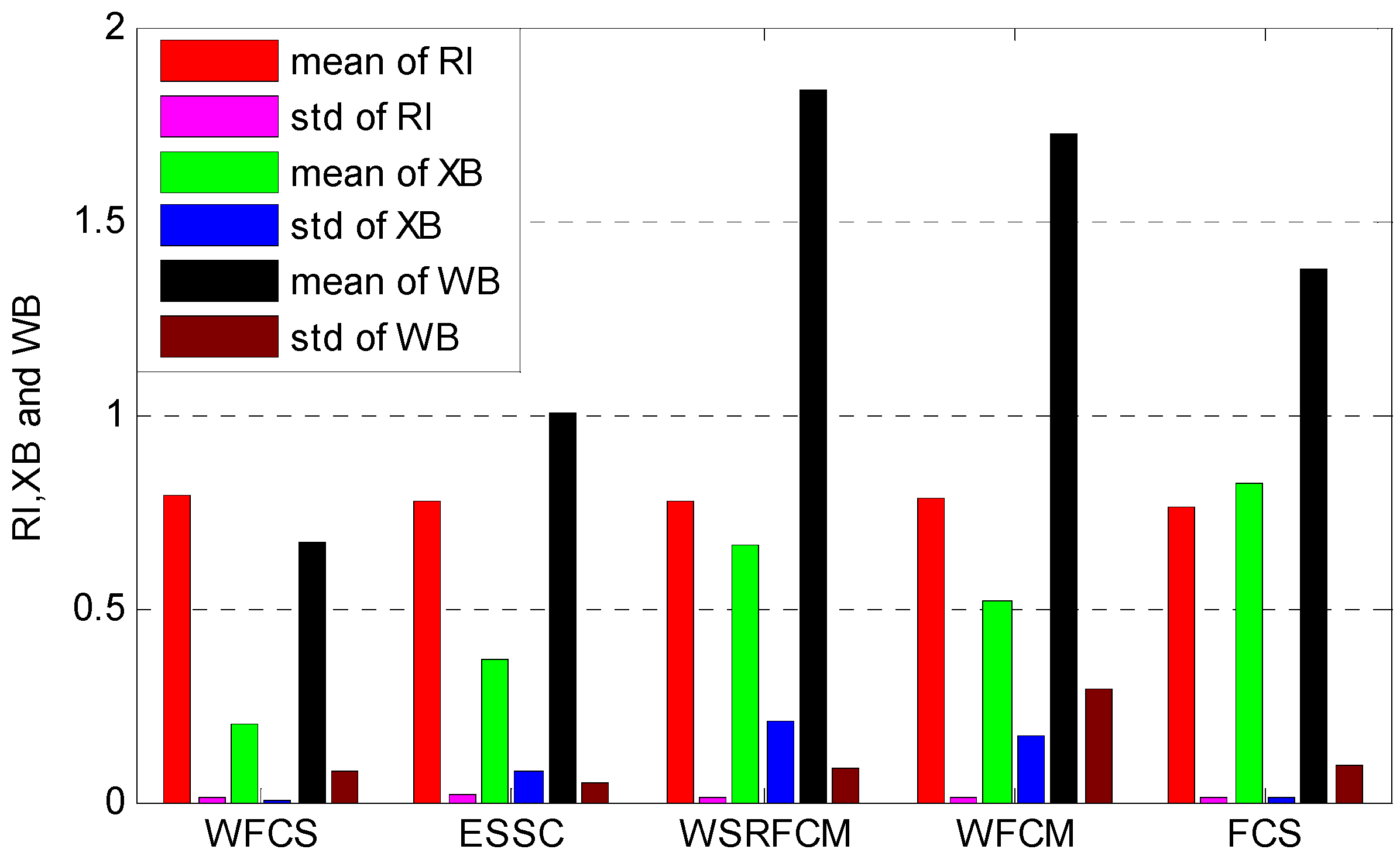
3.3. Clustering Evaluation

| Dataset | WFCS | ESSC | WSRFCM | WFCM | FCS |
|---|---|---|---|---|---|
| Australian | |||||
| mean | 0.7336 | 0.7162 | 0.7302 | 0.7265 | 0.6995 |
| std | 0.0000 | 0.1134 | 0.0033 | 0.0569 | 0.0125 |
| Breast Cancer | |||||
| mean | 0.8721 | 0.8779 | 0.8630 | 0.8600 | 0.8627 |
| std | 0.0009 | 0.0057 | 0 | 0.0000 | 0.0000 |
| Balance-scale | |||||
| mean | 0.6427 | 0.6389 | 0.6101 | 0.6099 | 0.6201 |
| std | 0.0758 | 0.0287 | 0.0586 | 0.0578 | 0.0662 |
| Heart | |||||
| mean | 0.7163 | 0.7114 | 0.7120 | 0.6939 | 0.6833 |
| std | 0.0000 | 0.0019 | 0.0023 | 0.0000 | 0.0000 |
| Iris | |||||
| mean | 0.9495 | 0.9195 | 0.9495 | 0.9495 | 0.8679 |
| std | 0.0000 | 0.0000 | 0.0081 | 0.0000 | 0.0000 |
| Pima | |||||
| mean | 0.5841 | 0.5564 | 0.5698 | 0.5837 | 0.5576 |
| std | 0.0000 | 0.0005 | 0.0044 | 0.0009 | 0.0000 |
| Vehicle | |||||
| mean | 0.6654 | 0.6539 | 0.6778 | 0.6581 | 0.6528 |
| std | 0.0025 | 0.0028 | 0.0006 | 0.0038 | 0.0000 |
| Wine | |||||
| mean | 0.9551 | 0.9398 | 0.9324 | 0.9398 | 0.9551 |
| std | 0.0000 | 0.0095 | 0.0000 | 0.0000 | 0.0000 |
| ENGINE | |||||
| mean | 0.8600 | 0.7823 | 0.7693 | 0.8600 | 0.7903 |
| std | 0.0000 | 0.0005 | 0.0067 | 0.0000 | 0.0000 |
| LTT | |||||
| mean | 0.9671 | 0.96 | 0.9543 | 0.9671 | 0.9607 |
| std | 0.0000 | 0.0000 | 0.0000 | 0.0000 | 0.0000 |
| Dataset | WFCS | ESSC | WSRFCM | WFCM | FCS |
|---|---|---|---|---|---|
| Australian | |||||
| mean | 0.0400 | 0.7194 | 1.4636 | 1.2056 | 0.1995 |
| std | 0.0007 | 0.3455 | 0.8407 | 1.0488 | 0.0267 |
| Breast Cancer | |||||
| mean | 0.3216 | 0.2961 | 0.4288 | 0.3270 | 0.1094 |
| std | 0.0021 | 0.0344 | 0.0903 | 0.0003 | 0.0000 |
| Balance-scale | |||||
| mean | 0.4435 | 0.7051 | 0.6970 | 0.7392 | 2.8475 |
| std | 0.0000 | 0.0248 | 0.0287 | 0.0725 | 0.0979 |
| Heart | |||||
| mean | 0.1593 | 0.4033 | 0.7942 | 0.6348 | 0.2267 |
| std | 0.0081 | 0.0982 | 0.7522 | 0.5030 | 0.0000 |
| Iris | |||||
| mean | 0.0844 | 0.0861 | 0.2700 | 0.1964 | 0.2922 |
| std | 0.0019 | 0.0059 | 0.0226 | 0.0000 | 0.0000 |
| Pima | |||||
| mean | 0.1443 | 0.4942 | 0.7610 | 0.5955 | 0.4759 |
| std | 0.0002 | 0.0235 | 0.1977 | 0.0406 | 0.0000 |
| Vehicle | |||||
| mean | 0.2532 | 0.2601 | 0.8538 | 0.5480 | 3.2949 |
| std | 0.0000 | 0.0917 | 0.0372 | 0.0047 | 0.0097 |
| Wine | |||||
| mean | 0.2577 | 0.3970 | 0.6775 | 0.4987 | 0.4061 |
| std | 0.0034 | 0.0009 | 0.0640 | 0.0000 | 0.0000 |
| ENGINE | |||||
| mean | 0.1699 | 0.1836 | 0.3755 | 0.2130 | 0.1267 |
| std | 0.0030 | 0.0685 | 0.0295 | 0.0217 | 0.0000 |
| LTT | |||||
| mean | 0.1019 | 0.1075 | 0.3299 | 0.2131 | 0.2105 |
| std | 0.0014 | 0.0983 | 0.0029 | 0.0000 | 0.0000 |
| Dataset | WFCS | ESSC | WSRFCM | WFCM | FCS |
|---|---|---|---|---|---|
| Australian | |||||
| mean | 0.0551 | 0.1730 | 0.6312 | 0.7261 | 0.5971 |
| std | 0.0000 | 0.1313 | 0.0011 | 0.4054 | 0.2144 |
| Breast Cancer | |||||
| mean | 0.3849 | 0.3843 | 0.5388 | 0.6035 | 0.4510 |
| std | 0.0010 | 0.0084 | 0.0000 | 0.0000 | 0.0000 |
| Balance-scale | |||||
| mean | 2.1924 | 3.6567 | 5.8354 | 6.1232 | 5.6191 |
| std | 0.7932 | 0.1983 | 0.0911 | 0.1686 | 0.7135 |
| Heart | |||||
| mean | 1.1191 | 1.1191 | 2.3297 | 3.3005 | 1.8087 |
| std | 0.0000 | 0.0991 | 0.0012 | 0.0000 | 0.0000 |
| Iris | |||||
| mean | 0.0729 | 0.3300 | 0.8423 | 0.6224 | 0.5366 |
| std | 0.0079 | 0.0097 | 0.6452 | 0.0311 | 0.0000 |
| Pima | |||||
| mean | 0.2828 | 0.6195 | 1.0043 | 0.4897 | 0.4832 |
| std | 0.0012 | 0.0003 | 0.0627 | 0.0073 | 0.0000 |
| Vehicle | |||||
| mean | 0.1908 | 0.2850 | 0.5000 | 0.4128 | 0.6351 |
| std | 0.0010 | 0.0087 | 0.0149 | 0.0000 | 0.0000 |
| Wine | |||||
| mean | 0.9821 | 0.9934 | 2.0174 | 1.4317 | 0.8599 |
| std | 0.0038 | 0.0350 | 0.0028 | 0.0000 | 0.0000 |
| ENGINE | |||||
| mean | 0.4866 | 0.8500 | 1.6315 | 1.6072 | 0.8484 |
| std | 0.0079 | 0.0060 | 0.0056 | 2.3408 | 0.0000 |
| LTT | |||||
| mean | 0.9206 | 1.6253 | 3.0179 | 1.9023 | 1.8894 |
| std | 0.0075 | 0.0281 | 0.0106 | 0.0002 | 0.0000 |
4. Conclusions
Acknowledgments
Author Contributions
Conflicts of Interest
References
- Hartigan, J. Clustering Algorithms; Wiley: New York, NY, USA, 1975. [Google Scholar]
- Jain, A.K.; Murty, M.N.; Flynn, P.J. Data clustering: A review. ACM Comput. Surv. (CSUR) 1999, 31, 264–323. [Google Scholar] [CrossRef]
- Xu, R.; Wunsch, D. Survey of clustering algorithms. Neu. Net. IEEE Transactions on 2005, 16, 645–678. [Google Scholar] [CrossRef]
- Bezdek, J.C. Pattern Recognition with Fuzzy Objective Function Algorithms; Plenum Press: New York, NY, USA, 1981. [Google Scholar]
- Wei, L.M.; Xie, W.X. Rival checked fuzzy c-means algorithm. Acta Electron. Sinica 2000, 28, 63–66. [Google Scholar]
- Fan, J.L.; Zhen, W.Z.; Xie, W.X. Suppressed fuzzy c-means clustering algorithm. Pattern Recognit. Lett. 2003, 24, 1607–1612. [Google Scholar] [CrossRef]
- Wu, K.L.; Yu, J.; Yang, M.S. A novel fuzzy clustering algorithm based on a fuzzy scatter matrix with optimality tests. Pattern Recognit. Lett. 2005, 26, 639–652. [Google Scholar] [CrossRef]
- Frigui, H.; Nasraoui, O. Unsupervised learning of prototypes and feature weights. Pattern Recognit. 2004, 37, 567–581. [Google Scholar] [CrossRef]
- Wang, X.; Wang, Y.; Wang, L. Improving fuzzy c-means clustering based on feature-weight learning. Pattern Recognit. Lett. 2004, 25, 1123–1132. [Google Scholar] [CrossRef]
- Jing, L.; Ng, M.K.; Huang, J.Z. An entropy weighting k-means algorithm for subspace clustering of high-dimensional sparse data. Knowl. Data Engin. IEEE Transactions on 2007, 19, 1026–1041. [Google Scholar] [CrossRef]
- Wang, Q.; Ye, Y.; Huang, J.Z. Fuzzy k-means with variable weighting in high dimensional data analysis. In Proceedings of Web-Age Information Management, 2008, WAIM'08. The Ninth International Conference on. Hunan, China; 2008; pp. 365–372. [Google Scholar]
- Wang, L.; Wang, J. Feature weighting fuzzy clustering integrating rough sets and shadowed sets. Int. J. Pattern Recognit. Artif. Intell. 2012, 26, 1769–1776. [Google Scholar]
- Deng, Z.; Choi, K.S.; Chung, F.L.; Wang, S.T. Enhanced soft subspace clustering integrating within-cluster and between-cluster information. Pattern Recognit. 2010, 43, 767–781. [Google Scholar] [CrossRef]
- Lichman, M. UCI Machine Learning Repository; University of California: Irvine, CA, USA, 2013. [Google Scholar]
- Rand, W.M. Objective criteria for the evaluation of clustering methods. J. Am. Stat. Assoc. 1971, 66, 846–850. [Google Scholar] [CrossRef]
- Xie, X.L.; Beni, G.A. A validity measure for fuzzy clustering. IEEE Trans. Pattern Anal. Mach. Intell. 1991, 13, 841–847. [Google Scholar] [CrossRef]
- Zhao, Q.; Fränti, P. WB-index: A sum-of-squares based index for cluster validity. Data Knowl. Eng. 2014, 92, 77–89. [Google Scholar] [CrossRef]
- Huang, J.Z; Ng, M.K; Rong, H.; Li, Z.C. Automated variable weighting in k-means type clustering. IEEE Trans. Pattern Anal. Mach. Intell. 2005, 27, 657–668. [Google Scholar] [CrossRef] [PubMed]
- Filippone, M.; Camastra, F.; Masulli, F.; Rovetta, S. A survey of kernel and spectral methods for clustering. Pattern Recognit. 2008, 41, 176–190. [Google Scholar] [CrossRef]
- Huang, H.C.; Chuang, Y.Y.; Chen, C.S. Multiple kernel fuzzy clustering. Fuzzy Syst. IEEE Transactions on 2012, 20, 120–134. [Google Scholar] [CrossRef]
- Lin, K.P. A Novel Evolutionary Kernel Intuitionistic Fuzzy C-means Clustering Algorithm. Fuzzy Syst. IEEE Transactions on 2014, 22, 1074–1087. [Google Scholar] [CrossRef]
© 2015 by the authors; licensee MDPI, Basel, Switzerland. This article is an open access article distributed under the terms and conditions of the Creative Commons Attribution license (http://creativecommons.org/licenses/by/4.0/).
Share and Cite
Zhou, Y.; Zuo, H.-f.; Feng, J. A Clustering Algorithm based on Feature Weighting Fuzzy Compactness and Separation. Algorithms 2015, 8, 128-143. https://doi.org/10.3390/a8020128
Zhou Y, Zuo H-f, Feng J. A Clustering Algorithm based on Feature Weighting Fuzzy Compactness and Separation. Algorithms. 2015; 8(2):128-143. https://doi.org/10.3390/a8020128
Chicago/Turabian StyleZhou, Yuan, Hong-fu Zuo, and Jiao Feng. 2015. "A Clustering Algorithm based on Feature Weighting Fuzzy Compactness and Separation" Algorithms 8, no. 2: 128-143. https://doi.org/10.3390/a8020128
APA StyleZhou, Y., Zuo, H.-f., & Feng, J. (2015). A Clustering Algorithm based on Feature Weighting Fuzzy Compactness and Separation. Algorithms, 8(2), 128-143. https://doi.org/10.3390/a8020128