A Study on the Fuzzy-Logic-Based Solar Power MPPT Algorithms Using Different Fuzzy Input Variables

Abstract

Maximum power point tracking (MPPT) is one of the key functions of the solar power management system in solar energy deployment. This paper investigates the design of fuzzy-logic-based solar power MPPT algorithms using different fuzzy input variables. Six fuzzy MPPT algorithms, based on different input variables, were considered in this study, namely (i) slope (of solar power-versus-solar voltage) and changes of the slope; (ii) slope and variation of the power; (iii) variation of power and variation of voltage; (iv) variation of power and variation of current; (v) sum of conductance and increment of the conductance; and (vi) sum of angles of arctangent of the conductance and arctangent of increment of the conductance. Algorithms (i)–(iv) have two input variables each while algorithms (v) and (vi) use a single input variable. The fuzzy logic MPPT function is deployed using a buck-boost power converter. This paper presents the details of the determinations, considerations of the fuzzy rules, as well as advantages and disadvantages of each MPPT algorithm based upon photovoltaic (PV) cell properties. The range of the input variable of Algorithm (vi) is finite and the maximum power point condition is well defined in steady condition and, therefore, it can be used for multipurpose controller design. Computer simulations are conducted to verify the design.

1. Introduction

Solar power is one of the most cleanest and abundant energy source in the world. It is virtually inexhaustible and is likely to be our main source of power in the future [1,2]. Solar power has already been widely applied for industrial, commercial, residential and military purposes. Solar power generated by solar or photovoltaic (PV) cells depends on the environmental conditions such as irradiations, sunlight incident angle, cell temperature, and load conditions. Power converters would be typically inserted between the PV cells and the load to control the power flow from the PV cells to the load. Many PV systems also employ some form of maximum power point tracking (MPPT) to maximize power output, with the MPPT function achieved through continuously adjusting the duty ratio command of the power switch in the power converter.

MPPT algorithms maximize power output by gradually increasing or decreasing the duty ratio of the power converter according to the PV cell output power versus the voltage curve or the current versus voltage curve. Commonly used MPPT techniques include the perturbing and observing method [3] and the incremental conductance method [4], both methods using fixed step size for the increment of the duty ratio command. If the step size is too small, the tracking process would be slowed. If the step size is too large, then the system may fluctuate about the maximum power point (MPP).

In order to automatically adjust step sizes, variable step sizing algorithms based on adaptive and artificial intelligent techniques such as fuzzy logic and adaptive neuro-fuzzy system were assessed [5,6,7,8,9,10,11,12,13,14,15,16,17,18,19,20,21]. Fuzzy logic controllers are characterized by their ability to imitate human thinking. Unlike traditional controllers, fuzzy controllers are able to use empirical methods or professional knowledge to design variable step size increments of duty ratio command for the power converter even without having an understanding of the mathematical model of the plant. Design considerations and effectiveness of the fuzzy MPPT algorithm depend on the input and output variables selected for the system. The output variable of the fuzzy MPPT algorithm would usually be the duty ratio command of the power switch for the power converter. However, there would be a number of different MPPT algorithm input variables to choose from based on the characteristics of the PV cells. The most commonly used input variables for the MPPT algorithms would be the slope of the power-versus-voltage (P-V) curve of the PV cell characteristics curves and changes of this slope [10,11,12,17]. In a previous study [9], P-V slope and variation of power $\mathrm{\Delta }{P}_{PV}$ were selected as the input variables, while another study [13,18] selected variations of power and voltage ($\mathrm{\Delta }{P}_{PV}$ and $\mathrm{\Delta }{V}_{PV}$) as the input variables instead. Other studies also used variations of power and current ($\mathrm{\Delta }{P}_{PV}$ and $\mathrm{\Delta }{I}_{PV}$) [14]. Previous investigations adopting the incremental conductance method used conductance and increment of conductance as the fuzzy input variables for MPP evaluation [15]. Another reported fuzzy MPPT algorithm used the sum of the arctangent of the conductance and arctangent of the conductance increment as the input variable [16]. Despite the numerous combinations for input variables selected, design considerations for the determination of fuzzy rules were usually not discussed in detail in the literature.

In this paper, we have focused upon the design of solar power MPPT algorithms. Special emphases were provided on the considerations for determining associated fuzzy rules for different fuzzy input variables. Six fuzzy MPPT algorithms, based on different input-variables, are considered in the study including: (i) P-V slope ($S=\mathrm{\Delta }{P}_{PV}/\mathrm{\Delta }{V}_{PV}$) and changes of the slope ($\mathrm{\Delta }S$); (ii) P-V slope and variation of the power ($\mathrm{\Delta }{P}_{PV}$); (iii) variation of power and variation of voltage ($\mathrm{\Delta }{V}_{PV}$); (iv) variation of power and variation of current ($\mathrm{\Delta }{I}_{PV}$); (v) sum of conductance and increment of the conductance $(I_{PV}/V_{PV}+d{I}_{PV}/d{V}_{PV})$; and (vi) sum of angle of conductance and angle of increment of the conductance $\left({\tan }^{-1}(I_{PV}/V_{PV})+{\tan }^{-1}(d{I}_{PV}/d{V}_{PV})\right)$. Algorithms (i)–(iv) used two input variables while algorithms (v) and (vi) used a single input variable. A MATLAB-based computer simulation program was developed to verify the fuzzy MPPT algorithms, with the algorithm verification results presented in this paper as well. A summary of the advantages and disadvantages of the six algorithms were also provided. Amongst these algorithms, algorithm (vi) had a well-defined input variable with finite range, as well as a well-defined MPP condition in stable conditions. Thus, algorithm (vi) could be formulated as a means of feedback control and applied in multipurpose controller designs.

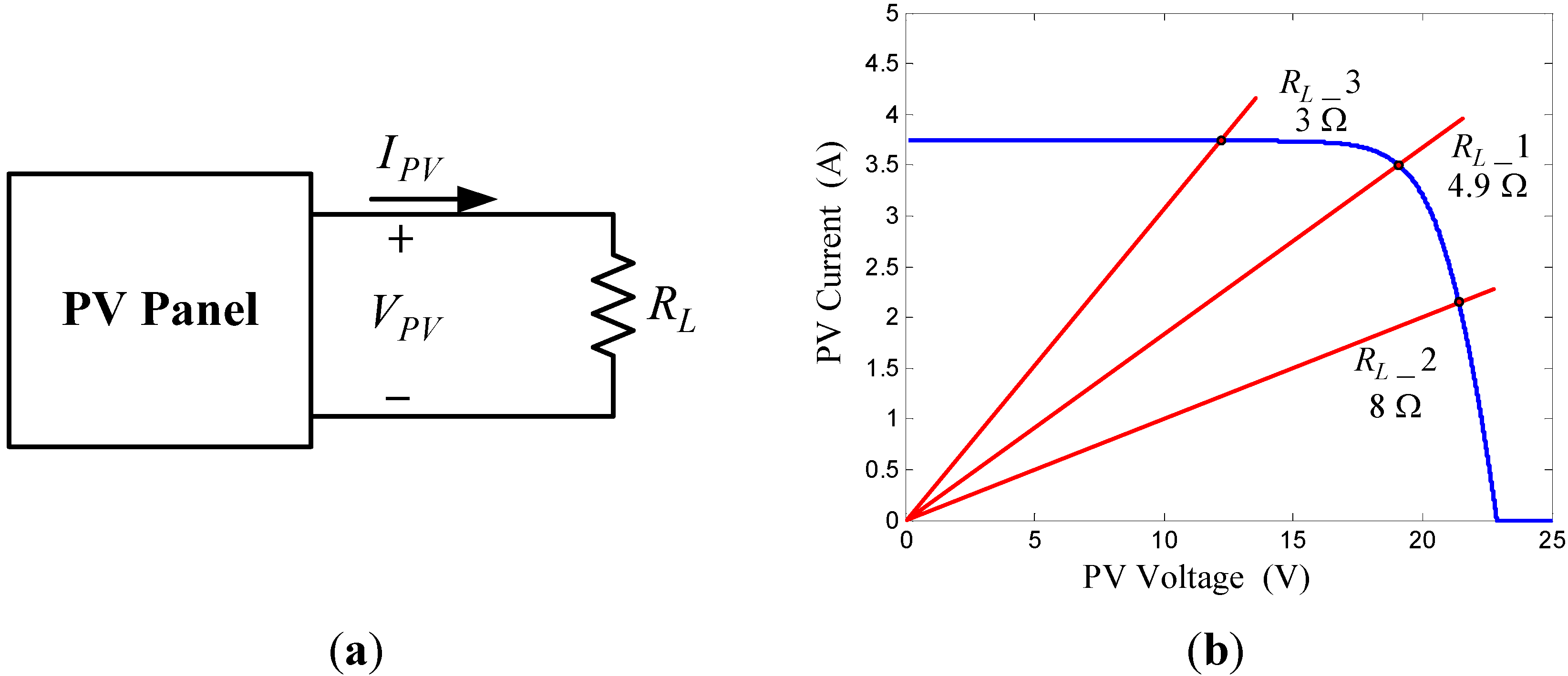
2. Solar Power MPPT System

The use of PV cells to generate solar power would depend on environmental conditions such as irradiation, sunlight incident angle, cell temperature, and the load conditions. The Solarex MSX60 PV panel was used in the design and analysis performed in this study. The characteristic output at 25 °C of this PV panel is shown in Figure 1. Figure 1a shows the relationship diagram between the PV cell power output and the voltage while Figure 1b shows the relationship diagram between the current and the voltage. To simplify the analysis, resistive load was considered in this study. Figure 2a shows the circuit diagram of using a PV cell panel for a resistive load $R_L$. Figure 2b shows the I-V characteristics of the system with an irradiation of $G=1$ $(1000{\text{ W/m}}^2)$ and temperature of 25 °C under different loads $R_L$. In Figure 2b, the intersection of the I-V characteristic curve (blue) of the PV panel and the $R_L$ I-V curve (red) would be the operating point of the system. From the figure, it could be seen that the operating point changes with changing load resistance $R_L$. The MPP may be achieved through proper selection of the load $R_L$. In most actual cases, loads tend to be less than optimal (in terms of maximum power delivered from the PV panel). Maximum power from the PV panel may be attained by incorporating an intelligent mechanism capable of altering the load resistance of the PV panel. Power converters were usually used to adjust the operating point of the PV system to maximize the power obtained from the system.

Figure 1. PV panel characteristics. (a) Power versus voltage; (b) Current versus voltage.

Figure 1. PV panel characteristics. (a) Power versus voltage; (b) Current versus voltage.

Figure 2. (a) PV system with resistive load; (b) I-V characteristics.

Figure 2. (a) PV system with resistive load; (b) I-V characteristics.

Figure 3 shows the block diagram of the MPPT system investigated in this study. This MPPT system included a PV panel, a buck-boost power converter, and an MPPT controller. Resistive load was considered in this study to simplify the analysis. The Zeta type buck-boost converter [22], as shown in Figure 4a, was used to control the power flow from the PV panel to the load. The terminal voltage of the PV system, $V_{PV}$, was very sensitive to the variation of the duty ratio command, $D$, of the power switch of the buck-boost converter. Maximum power could be achieved by properly adjusting the duty ratio command of the converter. Given that the purpose of this study was to maximize power output from the PV system, converter parameters were selected to operate the converter in continuous conducting mode. The parameters selected for this study are $L_1=L_2=470\text{ μH}$, $C_{IN}=C_2=1000\text{ μF}$, and $C_1=200\text{ μF}$. The PWM switching frequency is 200 kHz. Internal resistances of the components were ignored to obtain Equation (1) on the relationship between the converter input and output voltages in steady state:

$$V_{out}=\frac{D}{1-D}{V}_{PV}$$

(1)

By assuming that the converter operates at 100% efficiency with a resistive load $R_L$, the power delivered from this PV system would be:

$$P_{PV}={\left(\frac{D}{1-D}\right)}^2\frac{V_{PV}^2}{R_L}$$

(2)

Figure 4b shows P-V curves at different irradiation levels (blue lines) according to Equation (2) and different duty ratio commands (red lines) with $R_L=3\mathrm{\Omega }$. Intersections of the characteristic curves represent the operation points of the PV system. Thus, the operating point can be controlled by adjusting the duty ratio command of the buck-boost converter so as to achieve maximum power operation.

This study used the fuzzy theory to design the MPPT controller. Fuzzy MPPT controllers would generate fuzzy input variables needed by reading voltage and current signals from the PV cell. The fuzzy input variables would then be used to calculate the duty ratio command for adjusting the operating point of the PV cell in order to maximize the power output. Figure 5 shows the calculation process flowchart of the fuzzy controller. Fuzzy MPPT controller designs would differ based upon the choice of the fuzzy input variables and give rise to different effects on the MPPT process. Hence, the main purpose of this study would be to investigate the differences in the designs of fuzzy MPPT controllers using different fuzzy input variables.

Figure 3. Solar power maximum power point tracking system.

Figure 3. Solar power maximum power point tracking system.

Figure 4. (a) Zeta type buck-boost converter; (b) PV power characteristics.

Figure 4. (a) Zeta type buck-boost converter; (b) PV power characteristics.

Figure 5. Computation flow diagram of the fuzzy controller.

Figure 5. Computation flow diagram of the fuzzy controller.

3. Fuzzy MPPT algorithms

This study made a thorough investigation on common fuzzy input variables for fuzzy logic based MPPT algorithms by reviewing the characteristics of PV cells and past literature on fuzzy MPPT controller designs. Advantages and disadvantages of various designs were reviewed and provided with detailed discussions on issues encountered during the design process. Finally, the designs were verified using computer simulation.

Algorithm (i): P-V Slope and Variation of Slope as the Inputs

Algorithm (i) of the fuzzy logic MPPT system used the slope of the PV cell’s Power-Voltage (P-V) curve ($S(k)$) and variation of slope ($\mathrm{\Delta }S(k)$) as the fuzzy input variables. These variables were defined using the following equations:

$$S(k)=\frac{\mathrm{\Delta }{P}_{PV}}{\mathrm{\Delta }{V}_{PV}}=\frac{I_{PV}(k)\cdot V_{PV}(k)-I_{PV}(k-1)\cdot V_{PV}(k-1)}{V_{PV}(k)-V_{PV}(k-1)}$$

(3)

$$\mathrm{\Delta }S(k)=S(k)-S(k-1)$$

(4)

Figure 6 shows the database for fuzzy rules designed according to the fuzzy input variables. A five-term fuzzy set, positive big (PB), positive small (PS), zero (ZE), negative small (NS), and negative big (NB), is defined to describe each linguistic variable. Output from the fuzzy controller (duty ratio command of the buck-boost converter) would change the output voltage and current of the PV cell. Once PV cell outputs change, it would affect the values of the next round of fuzzy input variables. The controller would then re-adjust the output commands accordingly. According to fuzzy logic, the selection of the domain of the inputs and outputs (universe of discourse) will also directly affect the results, so careful designs must be implemented. The general guidelines for determining the membership functions are: (1) defining the boundaries of the PB and NB regions first based the characteristics of the input variables; (2) the range of ZE is then determined based on the predetermined MPPT goal (efficiency criteria); (3) the boundaries of PM and NM are then determined following the selection of the boundaries of PB, NB, and ZE. Design iterations are usually required to reach a satisfactory result. Figure 7 shows the corresponding input and output membership functions.

Figure 6. Fuzzy rules for P-V slope and changes of slope as the inputs.

Figure 6. Fuzzy rules for P-V slope and changes of slope as the inputs.

Figure 7. Membership functions for Algorithm (i): (a) Membership function for P-V slope, (b) Membership function for changes of slope; (c) Membership function for increment of duty ratio command.

Figure 7. Membership functions for Algorithm (i): (a) Membership function for P-V slope, (b) Membership function for changes of slope; (c) Membership function for increment of duty ratio command.

According to Figure 6, the fuzzy rule database was divided into three regions. The following provides detailed explanations on the design considerations for the rule database of each region.

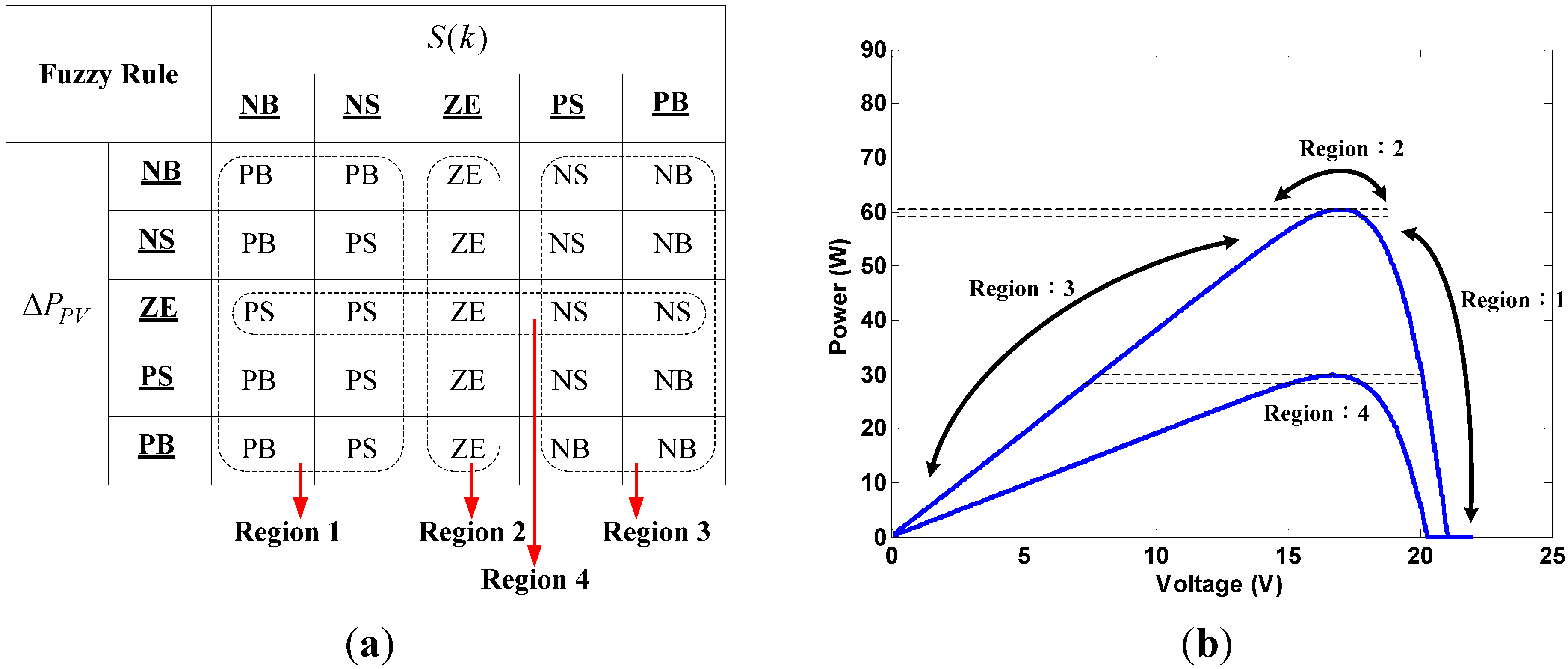
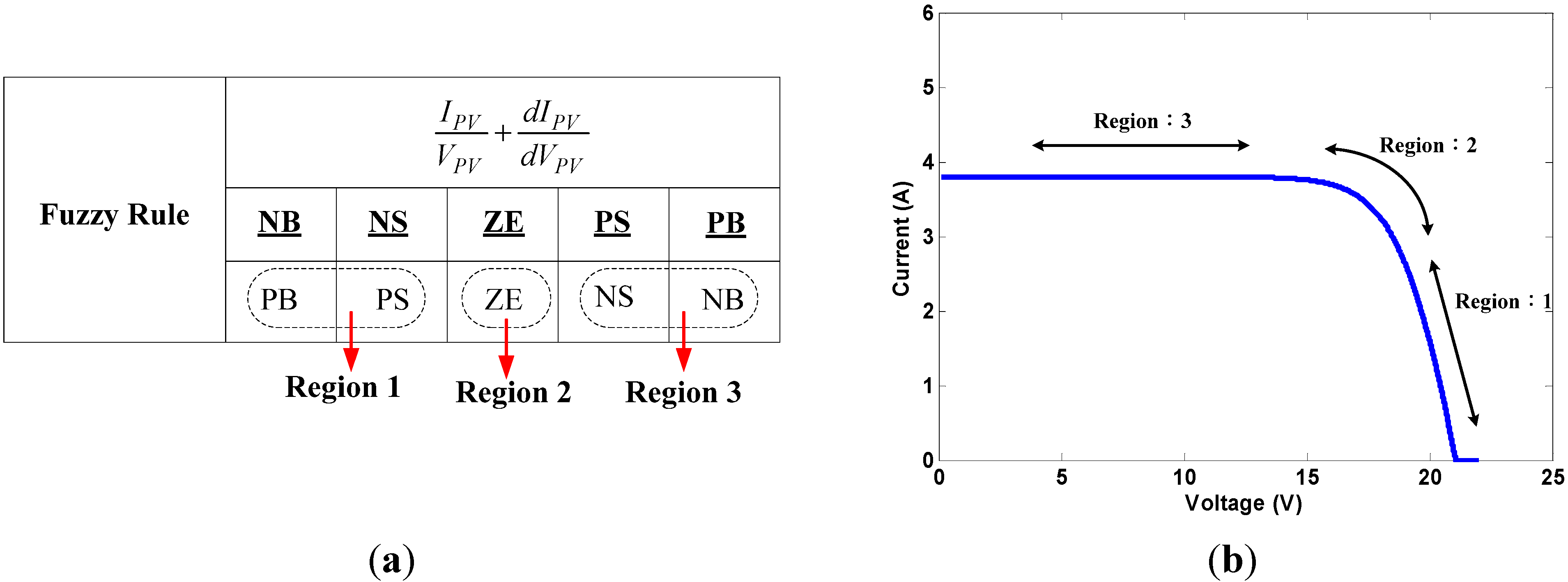
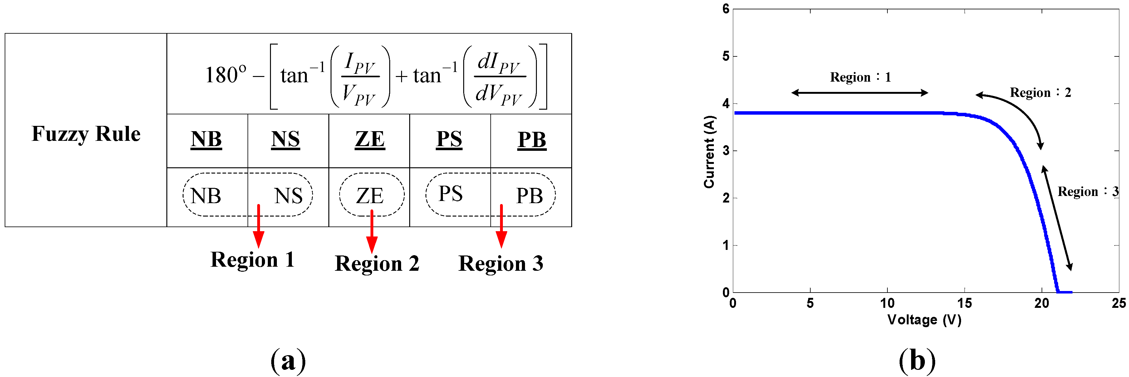
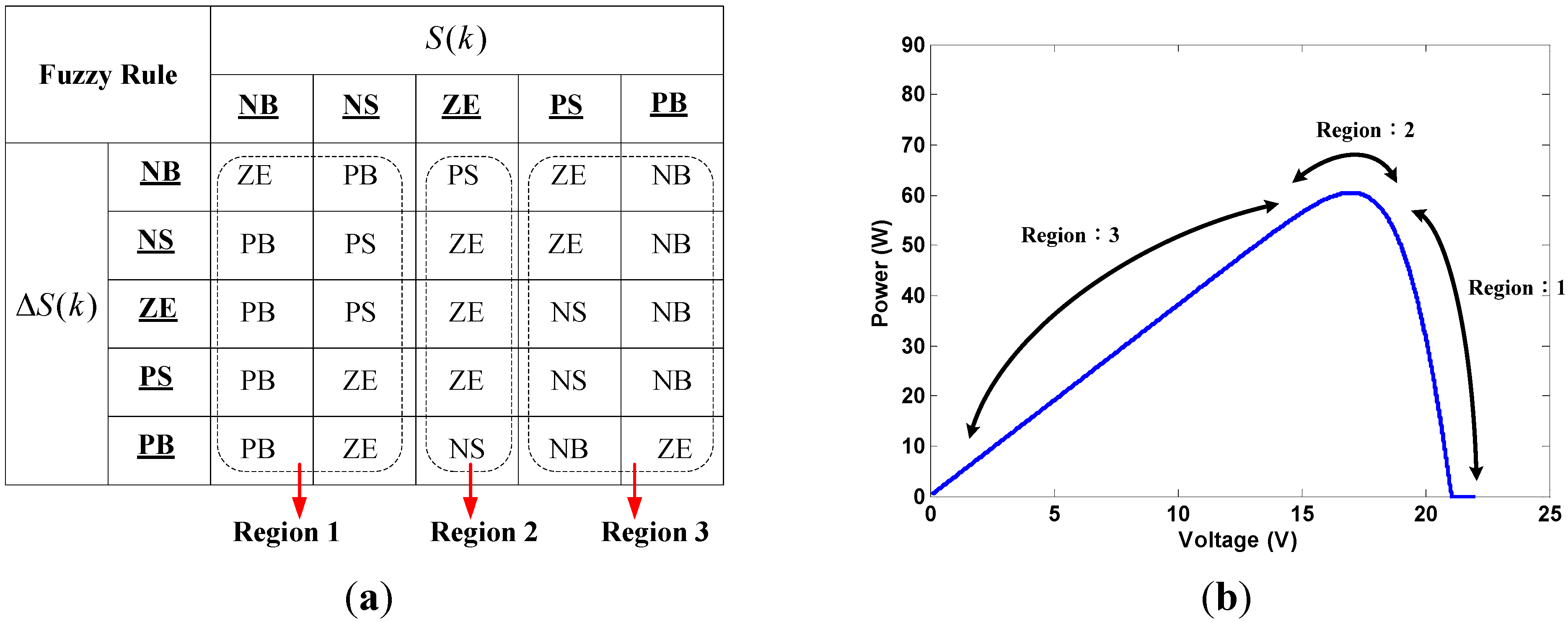
Region 1.

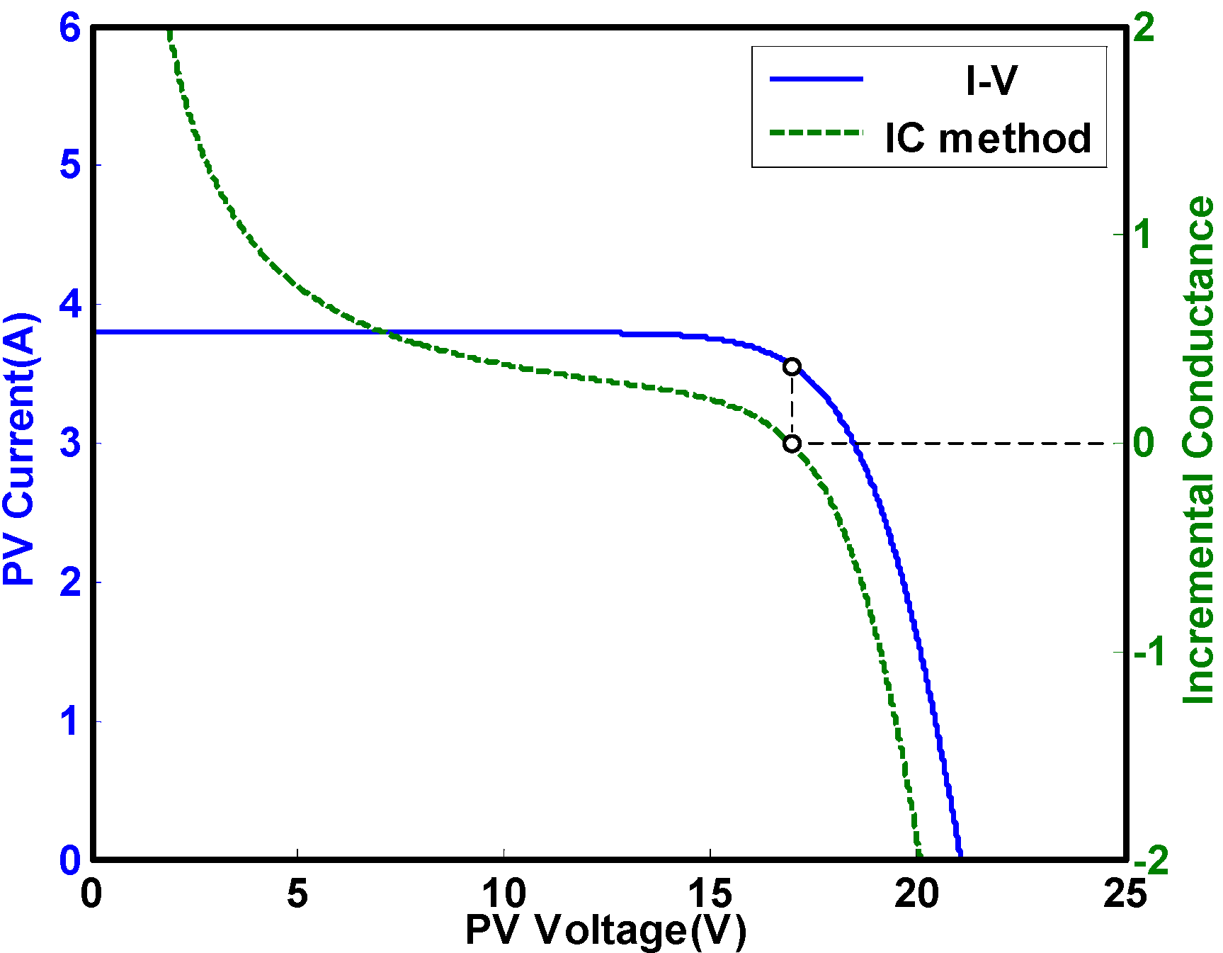
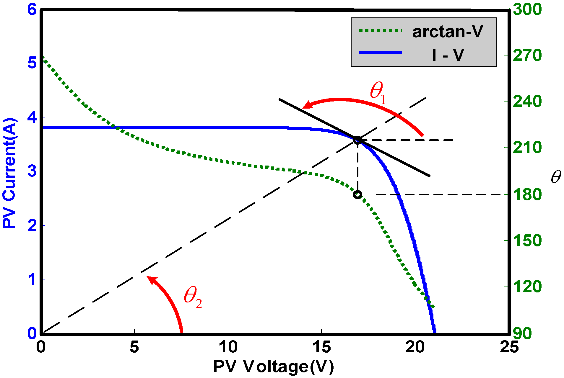
The slope is negative in this region, showing that the operating point of the PV cell is located on the right side of the MPP. At this time, duty ratio should be increased in order to track and achieve the MPP. The second set of input variables would be used to determine the magnitude of the duty ratio to be increased. However, when $S(k)$ and $\mathrm{\Delta }S(k)$ are both NB, the calculations may lead to the wrong outputs given that $S(k)=\mathrm{\Delta }{P}_{PV}/\mathrm{\Delta }{V}_{PV}$. When the operating point is close to the MPP with both $\mathrm{\Delta }{P}_{PV}$ and $\mathrm{\Delta }{V}_{PV}$ being very small values, output would be set as ZE in order to avoid $S(k)$ from becoming NB and generate error output after division. When $S(k)$ is NS and $\mathrm{\Delta }S(k)$ is either negative or zero, it would mean that the operating point would be located on the right side of the MPP and is tending to move to the right side further. Hence, the rule database was set to increase duty ratio under this condition. If $\mathrm{\Delta }S(k)$ is positive at this point, it would mean that the operating point is approaching the MPP from the right side. At this time, the output would be set to ZE in order to prevent over-increasing the duty ratio and causing the system to oscillate.

Region 2.

In this region, $S(k)$ is ZE, meaning that the operating point would be close to the MPP. Hence, the principle would be to maintain the same duty ratio under such conditions. If $\mathrm{\Delta }S(k)$ is NB, then the operating point would be rapidly approaching the MPP from the left side (duty ratio decreased). In order to prevent the operating point from moving to the right side of the MPP, the controller would use PS to suppress the change of magnitude of the duty ratio in the opposite direction. When $\mathrm{\Delta }S(k)$ is PB, the operating point would be located on the right side of the MPP. In order to prevent sudden over-increases of the duty ratio that may cause the operating point to cross-over to the left side of the MPP, the controller would use NS to suppress the magnitude of change of the duty ratio.

Region 3.

When $S(k)$ is positive, the operating point would be located on the left side of the MPP. Under such conditions, the duty ratio should be decreased for MPPT. A second set of input variables would be used to determine the magnitude of duty ratio to be decreased. When both $S(k)$ and $\mathrm{\Delta }S(k)$ are PB, the controller may generate the wrong outputs owing to the reasons similar to that with Region 1. Hence, the output should be set to ZE to avoid such conditions. When the system determines that $S(k)$ is PS and that $\mathrm{\Delta }S(k)$ is positive or zero, the operating point would be on the left side of the MPP and is tending to move to left further. The rule database would be set to reduce duty ratio under such conditions. When $\mathrm{\Delta }S(k)$ is negative at this point, the operating point would be approaching the MPP from the left side. At this time, the output would be set to ZE in order to prevent over-decreasing the duty ratio and system oscillation.

In order to verify the design of the fuzzy logic MPPT algorithm, a solar power MPPT simulation system was established on MATLAB as the verification model. As the MPPT system must be capable of maintaining normal operations during changing irradiations, the simulation system would therefore change irradiation levels every 0.2 seconds using the sequence $G=1\to 0.8\to 0.5\to 0.6\to 0.4$. Updating rate of the fuzzy controller was set to 100 Hz and the load resistance set to 8 $\mathrm{\Omega }$. Figure 8 shows the simulation results. Dotted red lines in the figure show the maximum power output under different irradiation. The marks with (X, Y) values show the steady state results. Y-value indicates power delivered from the PV panel. X-value is the corresponding instant of time. Results show that even with changing irradiation, the MPPT system was still capable of successfully tracking the MPP. Hence, this MPPT system design would be considered successful.

Figure 8. Simulation results using P-V slope and changes of slope as the inputs.

Figure 8. Simulation results using P-V slope and changes of slope as the inputs.

Algorithm (ii): P-V Slope and Variation of Power as the Inputs

Algorithm (ii) of the fuzzy logic MPPT system used the slope $S(k)$ and variation of power ($\mathrm{\Delta }{P}_{PV}$) as the fuzzy input variables. Figure 9 shows the database for fuzzy rules designed according to the fuzzy input variables. Figure 10 shows the corresponding input and output membership functions.

Figure 9. Fuzzy rules for P-V slope and variation of power as the inputs.

Figure 9. Fuzzy rules for P-V slope and variation of power as the inputs.

Figure 10. Membership functions for Algorithm (ii): (a). Membership function for P-V slope; (b) Membership function for changes of slope; (c). Membership function for increment of duty ratio command.

Figure 10. Membership functions for Algorithm (ii): (a). Membership function for P-V slope; (b) Membership function for changes of slope; (c). Membership function for increment of duty ratio command.

The fuzzy rules database was divided into 4 regions according to the characteristics of the P-V curve of the PV cell. Detailed analysis and discussions are provided below.

Region 1.

The main determinant in this region is a negative slope, with the operating point located on the right side of the MPP. Hence, the system is able to conclude that duty ratio needs to be increased to track the MPP. Variation to power output would be used to acquire the magnitude of increase for the duty ratio.

Region 2.

The slope is ZE in this region. Duty ratio would thus remain unchanged.

Region 3.

The main determinant in this region is a positive slope, with the operating point located on the left side of the MPP. Hence, the system is able to conclude that duty ratio needs to be decreased to track the MPP. Variation to power output would be used to acquire the magnitude of decrease for the duty ratio.

Region 4.

This region mainly determines the responses implemented when changes to the power output has been determined to be ZE. When variation to power is ZE, the operating point would be very close to the MPP. At this time, $S(k)$ could be used to improve the precision of the operating point. The use of $S(k)$ specifically targets low irradiation levels where the P-V curve has very low slope and that the system may be unable to accurately perform MPPT. Hence, the slope was used to improve the accuracy and precision of the system algorithm. The designed increment or decrease of each duty ratio would be small in order to prevent adding or removing too much duty ratio in a single step that could give rise to fluctuations of the operating point.

Simulation conditions similar to that used in the Algorithm (i) were used, with Figure 11 showing the simulation results. Results also indicate that the resulting MPPT system is a successful one.

Figure 11. Simulation results for Algorithm (ii).

Figure 11. Simulation results for Algorithm (ii).

Algorithm (iii): Variation of Power and Variation of Voltage as the Inputs

Algorithm (iii) of the fuzzy logic MPPT system used variations of the PV cell power output ($\mathrm{\Delta }{P}_{PV}$) and variations of voltage ($\mathrm{\Delta }{V}_{PV}$) as the fuzzy input variables. Figure 12 shows the designed fuzzy rules database for these fuzzy input variables. The basic concept of this algorithm was derived from the perturbing and observing method. Figure 13 shows the membership functions that correspond to the relevant inputs and outputs.

Figure 12. Fuzzy rules for Algorithm (iii) using $\mathrm{\Delta }P$ and $\mathrm{\Delta }V$ as the inputs.

Figure 12. Fuzzy rules for Algorithm (iii) using $\mathrm{\Delta }P$ and $\mathrm{\Delta }V$ as the inputs.

Figure 13. Membership functions for Algorithm (iii): (a) Membership function for P-V slope; (b) Membership function for changes of slope; (c) Membership function for increment of duty ratio command.

Figure 13. Membership functions for Algorithm (iii): (a) Membership function for P-V slope; (b) Membership function for changes of slope; (c) Membership function for increment of duty ratio command.

The fuzzy rules database was divided into 9 regions according to the characteristics of the P-V curve of the PV cell. Detailed analysis and discussions are provided below.

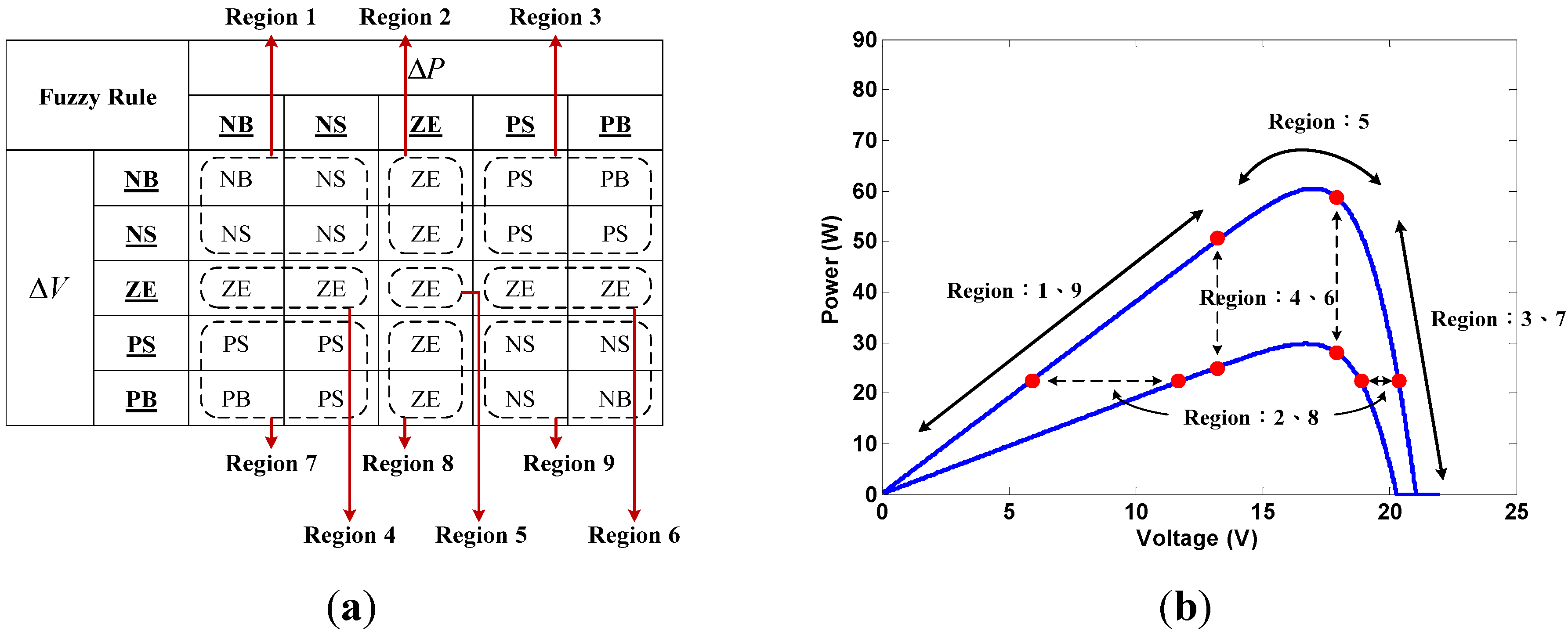
Region 1.

When both power and voltage decreases at the same time with the same irradiation, the operating point would be located on the left side of the MPP. Variations of the power and the voltage were used to determine the magnitude of decrease of the duty ratio.

Region 2.

Power remains unchanged but voltage has decreased. In such conditions, it would be assumed that the operating point would be at the MPP, thus giving an output of ZE. This algorithm would be unable to determine whether the irradiation has increased or decreased if irradiation has changed. The output would also be set at ZE in order to prevent contradictions.

Region 3.

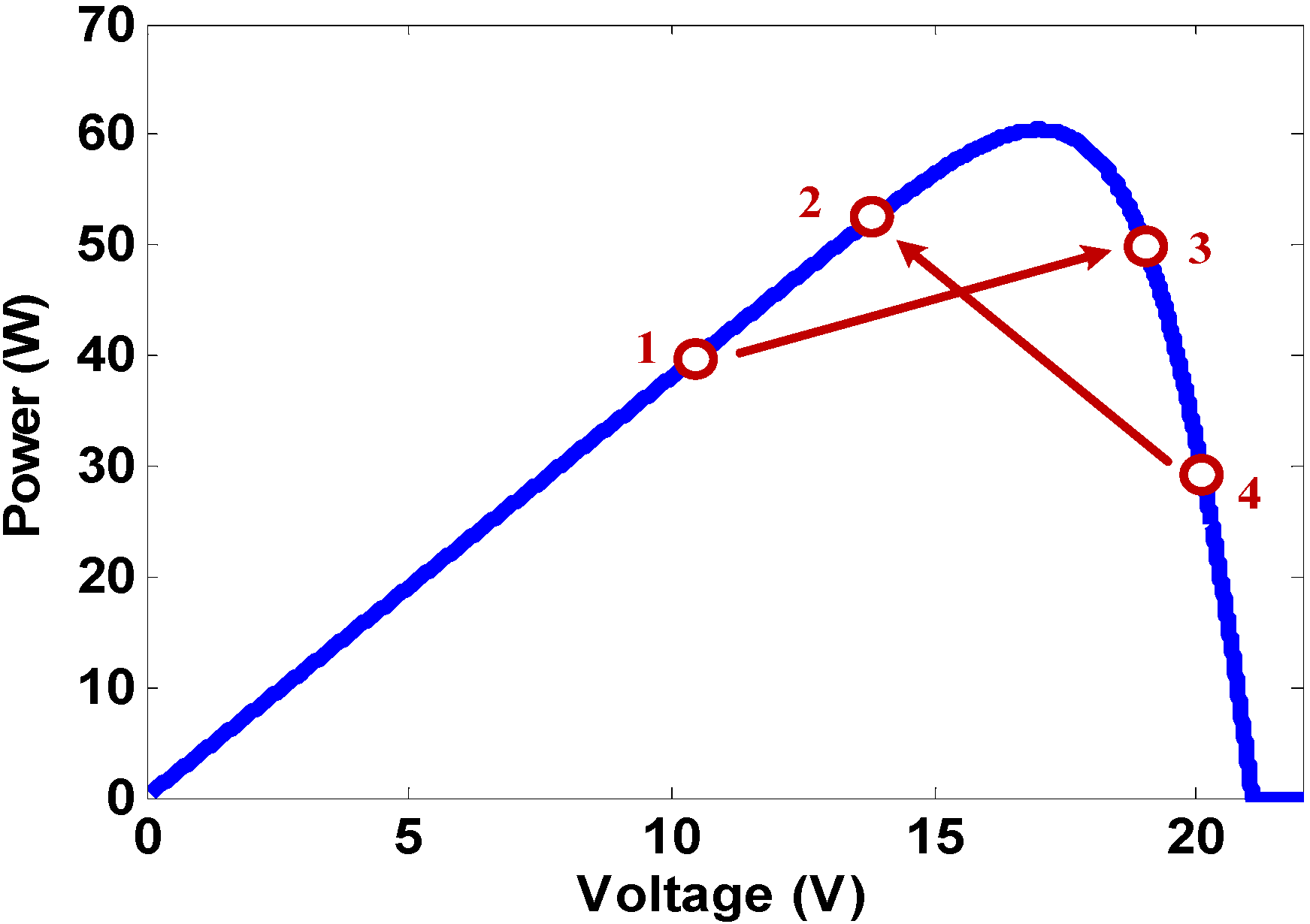
A region where irradiation remains unchanged, power increases, and voltage decreases. The operating point would be located on the right side of the MPP. At this time, variations of the power and voltage would be used to determine the magnitude of increases of the duty ratio. However, if the duty ratio command was an excessive increase causing the operating point to go from the right side of the MPP to its left side as shown in Figure 14 (going from Point 4 to Point 2), then a contradictory command would have been issued. Under such conditions, the power should increase and voltage should drop. However, after the duty ratio command, the operating point would relocated to the left side of the MPP, which meant that the duty ratio must be reduced in the MPPT process, contradicting the command for increasing the duty ratio in the fuzzy rules database. As this would cause the system to generate the wrong outputs and lead to fluctuations, the step size of the duty ratio cannot be too large.

Region 4.

This region is characterized by unchanging voltage but reducing power. Under such conditions, if the irradiation does not change, the system would be unable to determine whether the operating point is located on the left or right side of the MPP. Hence, the output of this region would be set as ZE. When irradiation changes, the algorithm would also be unable to determine whether the operating point is located on the left or right side of the MPP. Setting the output to ZE would prevent contradictions.

Region 5.

When both the power and voltage are no longer changing, it means that the system has managed to track and arrive at the MPP. Duty ratio would no longer be changed. The output in this region would be set as ZE.

Region 6.

In this region, power increases while voltage remains unchanged. When the irradiation does not change, the system would be unable to determine whether the operating point is located on the left or right of the MPP. Hence, this output of this region would be set as ZE. When the irradiation levels change, the algorithm would still be unable to determine whether the operating point is located on the left or right side of the MPP. Setting the output to ZE would prevent contradictions.

Region 7.

Where the irradiation does not change, power drops, and voltage increases. This condition indicates that the operating point is located on the right side of the curve. A relevant increase to the duty ratio would be implemented according to the changes to the power and voltage.

Region 8.

In this region, power remains unchanged while voltage increases. When irradiation remains unchanged, the MPP is assumed to have been reached. Hence, the output would be set as ZE. If irradiation has changed, this region would still be unable to determine whether the irradiation has increased or decreased. The output would also be set at ZE in order to prevent contradictions.

Region 9.

When both power and voltage increases at the same time with the same irradiation, it would mean that the operating point is located on the left side of the MPP. Changes to the power and voltage are used to determine the magnitude of decrease of the duty ratio. However, when the previous duty ratio command for decrease is excessive, the operating point may move from Point 1 to Point 3 as shown in Figure 14. After the shift, the power and voltage should both be increased, but the operating point would now be on the right side of the MPP, meaning that the duty ratio must be increased to track to the MPP, contradicting the need to reduce duty ratio command in the fuzzy rules database. As this would lead to system fluctuations, changes to duty ratio cannot be too high.

Figure 14. Example of rule conflictions for $\mathrm{\Delta }{P}_{PV}$ and $\mathrm{\Delta }{V}_{PV}$ as the inputs.

Figure 14. Example of rule conflictions for $\mathrm{\Delta }{P}_{PV}$ and $\mathrm{\Delta }{V}_{PV}$ as the inputs.

Figure 15 shows the computer simulation results of the fuzzy controller. Results from Figure 15 clearly indicate that the lower the irradiation, the poorer the tracking accuracy. Reducing the step sizes for the duty ratio commands would improve MPPT accuracy at lower irradiation levels. However, this meant that MPPT would take a longer time to accomplish. When comparing between the outputs, applying algorithm (iii) in MPPT would require longer tracking time and would thus have lower tracking efficiency compared to the two previous fuzzy controller algorithms.

Figure 15. Simulation results for Algorithm (iii).

Figure 15. Simulation results for Algorithm (iii).

Algorithm (iv): Variation of Power and Variation of Current as Inputs

Algorithm (iv) for the fuzzy logic MPPT is based on the PV cell output power versus current and duty ratio curve shown in Figure 16. Variations of the PV cell output power ($\mathrm{\Delta }{P}_{PV}$) and variations of the current ($\mathrm{\Delta }{I}_{PV}$) were used as the fuzzy input variables for the design of the fuzzy rule database. It could be seen from Figure 16 that the power versus current curve would have a similar shape to the power versus voltage curve. However, when the operating point is on the right side of the MPP, the power versus current curve exhibits a very steep slope. Further observations on the duty ratio clearly show that if the operating point is located on the right side of the MPP, it would be very sensitive to duty ratio changes. These characteristics severely impact the design and stability of the fuzzy controller. Figure 17 shows the fuzzy rules database designed using these fuzzy input variables. The corresponding membership functions of the outputs and inputs are shown in Figure 18.

Figure 16. PV cell power-current characteristics.

Figure 16. PV cell power-current characteristics.

Figure 17. Fuzzy rules for Algorithm (iv).

Figure 17. Fuzzy rules for Algorithm (iv).

Figure 18. Membership functions for Algorithm (iv): (a) Membership function for P-V slope; (b) Membership function for changes of slope; (c) Membership function for increment of duty ratio commands.

Figure 18. Membership functions for Algorithm (iv): (a) Membership function for P-V slope; (b) Membership function for changes of slope; (c) Membership function for increment of duty ratio commands.

Because algorithms (iii) and (iv) have similar input variables, and given the fact that current and voltage are inversely related, Algorithm (iv) can also be divided into 9 regions with opposite increase or decrease responses. The following describes the details.

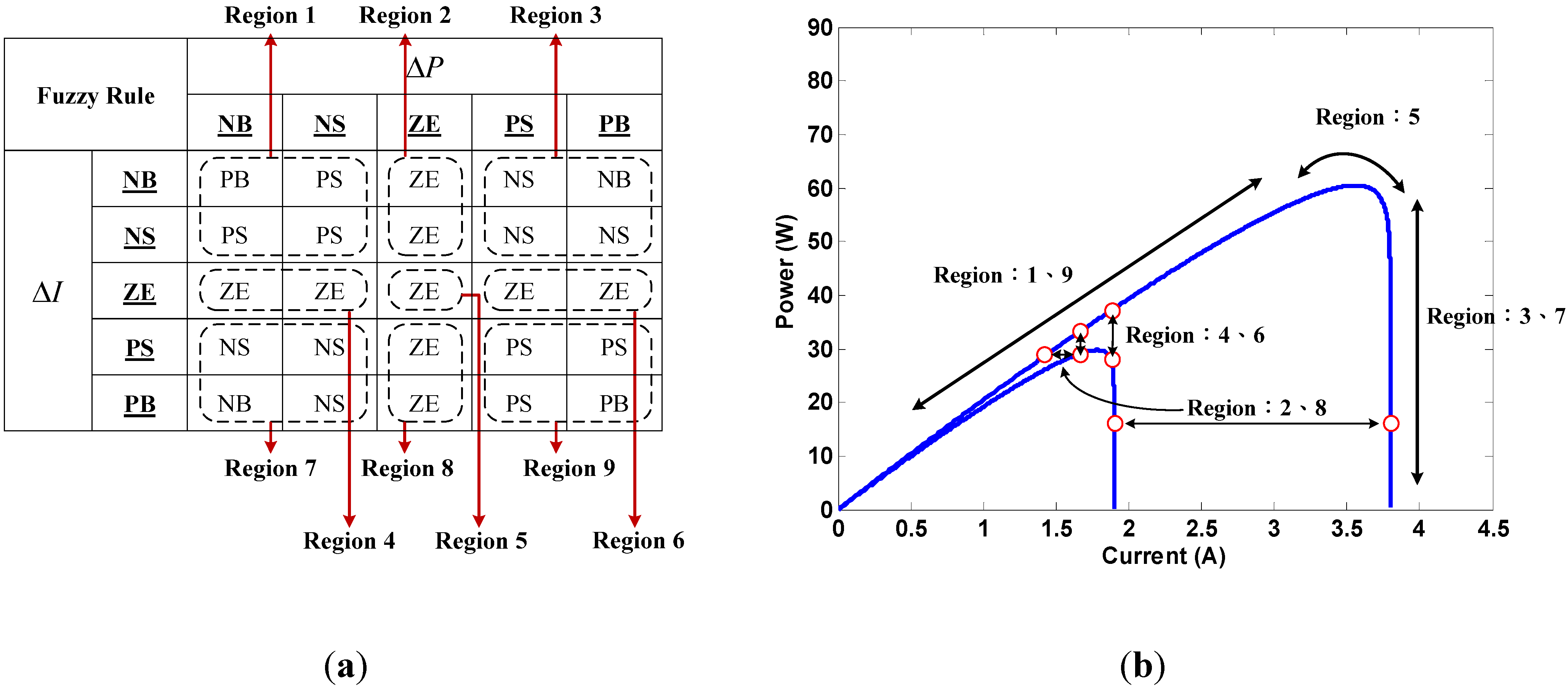
Region 1.

When both power and current decreases at the same time with the same irradiation, the operating point would be located on the left side of the MPP. Variations to the power and current would be used to determine the magnitude of increase of the duty ratio.

Region 2.

A region where power does not change but current has decreased. When irradiation remains unchanged, the MPP is assumed to have been reached. Hence, the output would be set as ZE. If irradiation has changed, this region would still be unable to determine whether the irradiation has increased or decreased. The output range would also be set at ZE in order to prevent contradictions.

Region 3.

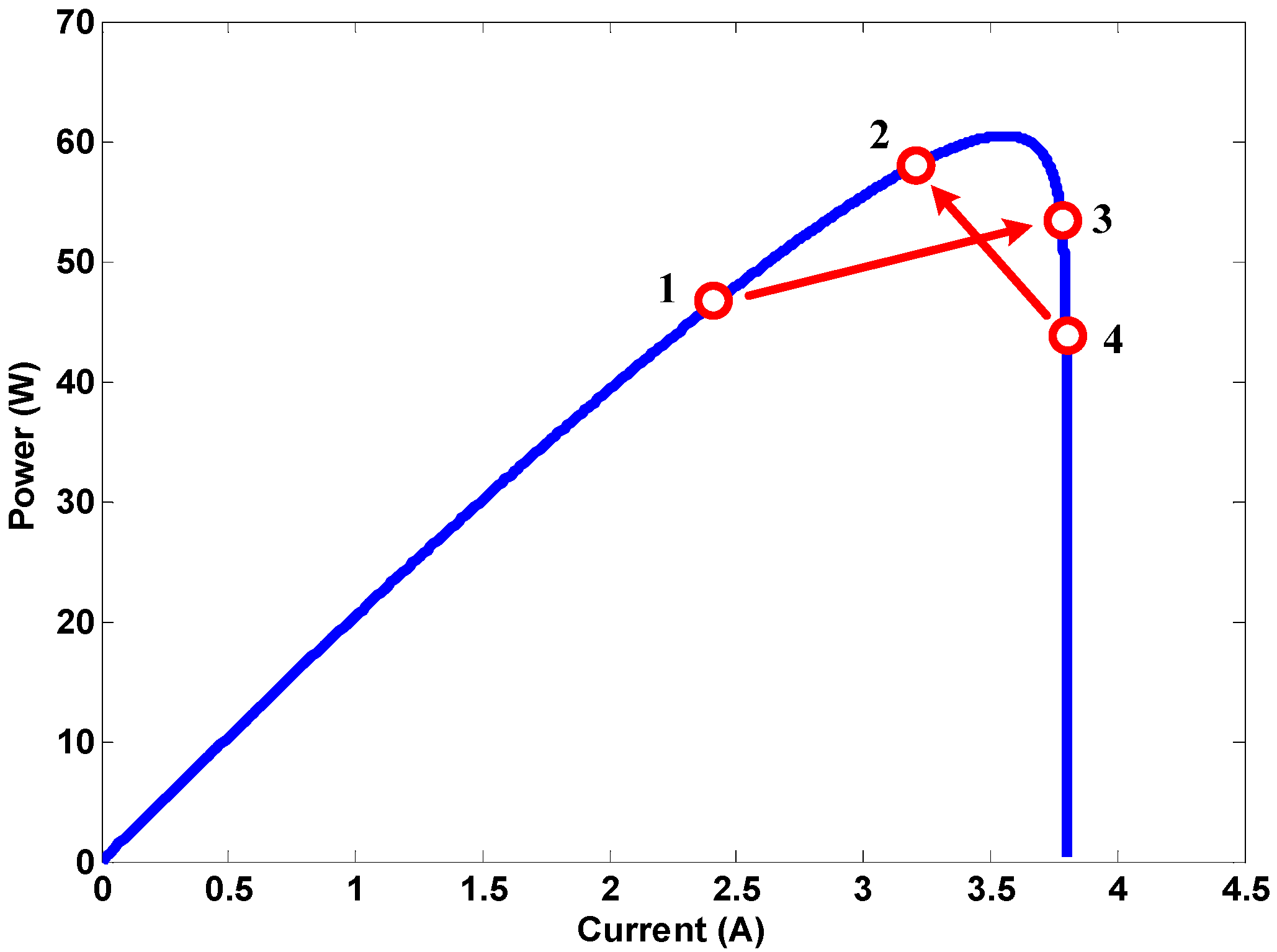
A region where irradiation remains unchanged, power increases, and current decreases. The operating point would be located on the right side of the MPP. At this time, changes to the power and current would be used to determine the magnitude of decreases of the duty ratio. However, if the duty ratio command was an excessive decrease that causes the operating point to go from Point 4 to 2 as shown in Figure 19, then a contradictory command would have been issued. After the command, the power should increase and current should drop. However, the operating point would now be located on the left side of the MPP, which meant that the duty ratio must be increased in order to track the MPP, contradicting the reduction of duty ratio commands in the fuzzy rules database. As this would cause the system to generate the wrong outputs and lead to fluctuations, each change step of the duty ratio must not be too large.

Region 4.

A region where current is the same but power has decreased. When the irradiation does not change, the system would be unable to determine whether the operating point is located on the left or right of the MPP. Hence, the output of this region would be set as ZE. When the irradiation changes, the system would still be unable to determine whether the operating point is located on the left or right side of the MPP. Setting the output to ZE would prevent contradictions.

Region 5.

When both the power and current are no longer changing, it means that the system has managed to track and arrive at the MPP. Duty ratio would no longer be changed. The output in this region would be set as ZE.

Region 6.

A region where current is the same but power has increased. When the irradiation does not change, the system would be unable to determine whether the operating point is located on the left or right of the MPP. Hence, the output of this region would be set as ZE. When the irradiation changes, the system would still be unable to determine whether the operating point is located on the left or right side of the MPP. Setting the output to ZE would prevent contradictions.

Region 7.

A region where irradiation remains unchanged, power decreases, and current increases. The operating point is located on the right side of the MPP. At this time, variations to the power and current would be used to determine the magnitude of decreases of the duty ratio.

Region 8.

A region where power does not change but current has increased. When irradiation remains unchanged, the MPP is assumed to have been reached. Hence, the output would be set as ZE. If irradiation has changed, this region would still be unable to determine whether the irradiation has increased or decreased. The output would also be set at ZE in order to prevent contradictions.

Region 9.

When both power and current increases at the same time with the same irradiation, the operating point would be located on the left side of the MPP. Variations to the power and current would be used to determine the magnitude of increase of the duty ratio. However, if the duty ratio command was an excessive increase causing the operating point to go from Point 1 to 3, as shown in Figure 19, then a contradictory command would have been issued. After the command, both the power and current should increase. However, the operating point would now be located on the right side of the MPP, which meant that the duty ratio must be decreased in order to track the MPP, contradicting the command for increasing the duty ratio in the fuzzy rules database. As this would cause the system to generate the wrong outputs and lead to fluctuations, the duty ratio step size must not be too large.

Figure 19. Example of rule conflictions for $\mathrm{\Delta }{P}_{PV}$ and $\mathrm{\Delta }{I}_{PV}$ s the inputs.

Figure 19. Example of rule conflictions for $\mathrm{\Delta }{P}_{PV}$ and $\mathrm{\Delta }{I}_{PV}$ s the inputs.

Two issues have been identified when designing this algorithm. The first issue could be observed from the power to current and duty ratio curve shown in Figure 16. When the operating point is located at the right side of the MPP, it may be extremely sensitive to duty ratio commands. Hence, duty ratio step sizes cannot be too large to avoid falling into the short circuit current range. Hence, MPPT using this algorithm must be performed slowly. The second issue would be that the operating point may easily fall into the short circuit current range when the irradiation level is decreasing. Hence, when the current is not changing, the fuzzy rules would set the output as ZE to prevent the algorithm from tracking the MPP as shown in Figure 20. According to the simulation results shown in Figure 21, it could be observed that the MPPT at low irradiation may be incapable of tracking the operating point to the MPP. Under low irradiation levels, the operating point may easily reach a short-circuit current. If variation of current is zero, the fuzzy controller system would not change the duty ratio command as the system would have determined that the MPP has already been reached.

Figure 20. A diagram illustrating how the power versus current curve changes with irradiation.

Figure 20. A diagram illustrating how the power versus current curve changes with irradiation.

Figure 21. Variable $\text{Δ}P-\text{Δ}I$ power tracking results 1.

Figure 21. Variable $\text{Δ}P-\text{Δ}I$ power tracking results 1.

However, if the same set of fuzzy controller was used, when irradiation increases only, for example, $G=0.6\to 0.7\to 0.8\to 0.9\to 1$, the result would be as shown in Figure 22. From this figure, it could be seen that under increasing irradiation levels, the fuzzy controller would be capable of carrying out proper MPPT.

Figure 22. Variable $\text{Δ}P-\text{Δ}I$ power tracking results 2.

Figure 22. Variable $\text{Δ}P-\text{Δ}I$ power tracking results 2.

Algorithm (v): Sum of Conductance and Increment of Conductance as the Input

Algorithm (v) for the fuzzy logic MPPT algorithm would use incremental conductance as the basis for the fuzzy controller design. According to the P-V curve, the power to voltage derivative would be zero at the MPP condition:

$$\frac{d{P}_{PV}}{d{V}_{PV}}=0\Rightarrow I_{PV}+V_{PV}\frac{d{I}_{PV}}{d{V}_{PV}}=0\Rightarrow \frac{I_{PV}}{V_{PV}}+\frac{d{I}_{PV}}{d{V}_{PV}}=0$$

(5)

Figure 23 shows the characteristic P-V curve and the corresponding $I_{PV}/V_{PV}+d{I}_{PV}/d{V}_{PV}$ value. Algorithm (v) uses this special characteristic in designing the fuzzy controller. The unique feature of this algorithm was when $I_{PV}/V_{PV}+d{I}_{PV}/d{V}_{PV}>0$, the operating point would on the left side of the MPP on the P-V curve. In other words, when output voltage of the PV cell becomes too low, the system must reduce duty ratio commands in order to raise the PV cell output voltage. If $I_{PV}/V_{PV}+d{I}_{PV}/d{V}_{PV}<0$, the operating point would be on the right side of the MPP of the P-V curve. In other words, when PV cell output voltage becomes too high, the system must increase duty ratio commands in order to reduce the PV cell output voltage. This algorithm would provide the operating region of the PV cell. Only a single fuzzy input variable would be needed for the design of the fuzzy logic MPPT controller. Figure 24 shows the fuzzy rules database designed using this algorithm. The corresponding membership functions of the inputs and input are shown in Figure 25.

Figure 23. PV cell current-voltage and $I_{PV}/V_{PV}+d{I}_{PV}/d{V}_{PV}$ characteristics.

Figure 23. PV cell current-voltage and $I_{PV}/V_{PV}+d{I}_{PV}/d{V}_{PV}$ characteristics.

Figure 24. Fuzzy rules for Algorithm (v).

Figure 24. Fuzzy rules for Algorithm (v).

Figure 25. Membership functions for Algorithm (v): (a) Membership function for $I_{PV}/V_{PV}+d{I}_{PV}/d{V}_{PV}$, (b) Membership function for increment of duty ratio command.

Figure 25. Membership functions for Algorithm (v): (a) Membership function for $I_{PV}/V_{PV}+d{I}_{PV}/d{V}_{PV}$, (b) Membership function for increment of duty ratio command.

This algorithm allows the system to directly identify the location of the operating point in relation to the MPP unlike previous algorithms described in this paper where variations were used to estimate whether the system has tracked the operating point to the MPP instead. Hence, when using this algorithm in designing the output variable, duty ratio increments or decreases could be designed with larger values in order to achieve efficient MPPT. The other advantage is that this algorithm would not require the use of a second set of MPPT input variables, allowing the design of a single-input and single-output system which could reduce computing loads. The rules database for this algorithm is divided into 3 regions. Detailed analysis and discussions are provided below.

Region 1.

The operating point is located at the right of the MPP. The proximity of the operating point to the MPP is used to determine the degree of increase the duty ratio for the MPPT process.

Region 2.

The operating point is located near the MPP. The output is thus set as ZE.

Region 3.

The operating point is located at the left of the MPP. The proximity of the operating point to the MPP is used to determine the degree of decrease of the duty ratio for the MPPT process.

Figure 26 shows the simulation results of using this single-input fuzzy MPPT controller. Results show that under changing irradiation, this algorithm was capable of achieving MPP quickly. The process of this algorithm in locating the operating point was also more direct compared to the previous methods, and would not require the use of variations in input variables to predict operating point locations. However, the determination condition $I_{PV}/V_{PV}+d{I}_{PV}/d{V}_{PV}$ would become extremely sensitive near the MPP. Hence, the detection system must accurately calculate the determination results in order to track the operating point to the MPP, requiring the proper designs of the fuzzy domains and good precision of the measurement instruments used which could pose significant challenges to the design of this fuzzy controller. Additionally, extremely large or small values may possibly result from using this determination formula after division operations, making it important to perform detailed calculations.

Figure 26. Simulation results for Algorithm (v).

Figure 26. Simulation results for Algorithm (v).

Algorithm (vi): Sum of Angle Conductance and Angle of Increment of Conductance as the Input

Algorithm (vi), the final fuzzy logic MPPT algorithm discussed in this study, is a derived from Algorithm (v). The MPP determination condition of formula (5) was changed per Figure 27 to give:

$$\tan {\theta }_1=\frac{d{I}_{PV}}{d{V}_{PV}}\text{ , }\tan {\theta }_2=\frac{I_{PV}}{V_{PV}}$$

(6)

After simple geometric calculations, the determination conditions for maximum power of the PV cell could be rewritten as:

$${\theta }_1+{\theta }_2={\tan }^{-1}\left(\frac{d{I}_{PV}}{d{V}_{PV}}\right)+{\tan }^{-1}\left(\frac{I_{PV}}{V_{PV}}\right)={180}^{\text{o}}$$

(7)

The advantage of this determination method is placing a limit on the range of ${\text{θ}}_1+{\text{θ}}_2$, namely ${90}^{\text{o}}\le {\text{θ}}_1+{\text{θ}}_2\le {270}^{\text{o}}$. In Algorithm (v), the MPP determination range, $-\infty <I_{PV}/V_{PV}+d{I}_{PV}/d{V}_{PV}<\infty$, has no limits. Hence, it would be relatively easier to determine the universe of discourse of the input variable in Algorithm (vi) and that the MPP determination conditions would not be overly sensitive when the operating point approaches the MPP, all of which would facilitate the design of the fuzzy controller. Figure 28 shows the fuzzy rules database designed using these properties. The corresponding membership functions of the outputs and inputs are shown in Figure 29.

Figure 27. A concept diagram showing the corresponding Current ‒$\text{θ}$—Voltage.

Figure 27. A concept diagram showing the corresponding Current ‒$\text{θ}$—Voltage.

Figure 28. Fuzzy rules for Algorithm (vi).

Figure 28. Fuzzy rules for Algorithm (vi).

Figure 29. Membership functions for Algorithm (vi): (a) Membership function for ${\text{θ}}_1+{\text{θ}}_2$ (b) Membership function for increment of duty ratio command.

Figure 29. Membership functions for Algorithm (vi): (a) Membership function for ${\text{θ}}_1+{\text{θ}}_2$ (b) Membership function for increment of duty ratio command.

Like Algorithm (v), Algorithm (vi) also allows the system to directly identify the location of the operating point in relation to the MPP unlike Algorithms (i)~(iv) where variations were used to estimate whether the system has tracked the operating point to the MPP. Hence, the use of this algorithm in designing output domains allows greater step sizes in duty ratios that improve the efficiency of the MPPT process. The other advantage is that this algorithm would not require the system to use a second set of MPPT input variables. Hence, a single-input and single-output system could be designed in order to reduce computing loads. The rules database for this algorithm is divided into three regions. Detailed analysis and discussions are provided below.

Region 1.

The operating point is located at the left of the MPP. The proximity of the operating point to the MPP is used to determine the degree of decrease of the duty ratio for the MPPT process.

Region 2.

The operating point is located at the MPP. Output would be set to ZE.

Region 3.

The operating point is located at the right of the MPP. The proximity of the operating point to the MPP is used to determine the degree of increase the duty ratio for the MPPT process.

Figure 30 shows the results of the computer simulation. Under changing irradiation levels, this algorithm was capable of performing MPPT and reaching a stable operating point quickly. This algorithm was also capable of directly locating the operating point without the need to predict variations in the input variables, thus allowing a faster tracking speed. According to the results described above, Algorithm (vi) offers the fastest MPPT speed and easiest designs. However, calculations must be carried out carefully as ${\tan }^{-1}\left(d{I}_{PV}/d{V}_{PV}\right)$ and ${\tan }^{-1}\left(I_{PV}/V_{PV}\right)$ calculations must be performed for the input variables in addition to division operations.

Figure 30. Simulation results for Algorithm (vi).

Figure 30. Simulation results for Algorithm (vi).

The above contents described the six types of MPPT algorithms used. Advantages and disadvantages of these algorithms are summarized in Table 1. The summary of the simulation results including the efficiency and tracking speed information are given in Table 2.

Another common factor that affects the power variation is surface temperature of the solar cells. The characteristics of the PV power variations due to temperature changes are similar to the effect of irradiation changes. The advantages and disadvantages of the algorithms under temperature changes are the same as discussed in Table 1.

Table 1. Advantages and disadvantages of the MPPT algorithms.

Input Variables	Advantages	Disadvantages
Algorithm (i): P-V slope and changes of slope	Easily determines if the operating point is to the left or right of the MPP, facilitating the increase or decrease of the duty ratio. Changes to the slope can be used to determine the movement direction of the operating point to prevent fluctuations.	Given that the slope is $\mathrm{\Delta }{P}_{PV}/\mathrm{\Delta }{V}_{PV}$, near the MPP, both values would be very close to each other and very small as well, leading to possibility of output errors and subsequent fluctuations. At low irradiation, precision of MPPT would not be as high.
Algorithm (ii): P-V slope and $\mathrm{\Delta }{P}_{PV}$	Easily determines if the operating point is to the left or right of the MPP, facilitating the increase or decrease of the duty ratio. At low irradiation levels, $\mathrm{\Delta }{P}_{PV}$ can be used to determine changes to irradiation and facilitate tracking speed.	Fuzzy signal $\mathrm{\Delta }{P}_{PV}/\mathrm{\Delta }{V}_{PV}$ may have issues of wrong judgment, which may lead to subsequent fluctuations.
Algorithm (iii): $\mathrm{\Delta }{P}_{PV}$ and $\mathrm{\Delta }{V}_{PV}$	Designed according to changes in power and voltage based on the P-V curve to offer a very direct approach.	Unable to respond quickly during moments of changing irradiation. Both inputs are changes to variables, and would not be able to correctly identify the operating points. Each increment step to duty ratio cannot be too high, which means that tracking will be slower. At low irradiation, precision of MPPT would not be as high.
Algorithm (iv): $\mathrm{\Delta }{P}_{PV}$ and $\mathrm{\Delta }{I}_{PV}$	Applicable in non-changing irradiation in tracking or when the irradiation is increasing. Designed according to changes in current and voltage based on the P-I curve to offer a very direct approach.	Unable to respond quickly during moments of changing irradiation. Both inputs are changes to variables, and would not be able to correctly identify the operating points. Increment and decrease steps for the duty ratio cannot be too high, which meant that tracking would be slower. Operating point may easily fall to short circuit current ranges during moments of irradiation change. At low irradiation, precision of MPPT would not be as high.
Algorithm (v): $\frac{I_{PV}}{V_{PV}}+\frac{d{I}_{PV}}{d{V}_{PV}}$	Can be designed as a single-input and single-output system with simple design considerations. Can be rapidly tracked to the MPP. Able to directly locate the position of the operating point. Ensures that the error between curves of different irradiation would not be too big.	$d{I}_{PV}/d{V}_{PV}$, issue of division calculations. Sensitive to changes. Sensors must be sensitive enough, otherwise the algorithm will be unable to track the MPP.
Algorithm (vi): $\begin{array}{l}{\tan }^{-1}\left(\frac{I_{PV}}{V_{PV}}\right)+\\ {\tan }^{-1}\left(\frac{d{I}_{PV}}{d{V}_{PV}}\right)\end{array}$	Can be designed as a single-input and single-output system with simple design considerations. Can be rapidly tracked to the MPP. Able to directly locate the position of the operating point. Ensures that the error between curves of different irradiation would not be too big.	$d{I}_{PV}/d{V}_{PV}$, issue of division calculations Since arctangent calculations must be performed, the amount of computing required would be greater.

Table 1. Advantages and disadvantages of the MPPT algorithms.

Input Variables	Advantages	Disadvantages
Algorithm (i): P-V slope and changes of slope	Easily determines if the operating point is to the left or right of the MPP, facilitating the increase or decrease of the duty ratio. Changes to the slope can be used to determine the movement direction of the operating point to prevent fluctuations.	Given that the slope is $\mathrm{\Delta }{P}_{PV}/\mathrm{\Delta }{V}_{PV}$, near the MPP, both values would be very close to each other and very small as well, leading to possibility of output errors and subsequent fluctuations. At low irradiation, precision of MPPT would not be as high.
Algorithm (ii): P-V slope and $\mathrm{\Delta }{P}_{PV}$	Easily determines if the operating point is to the left or right of the MPP, facilitating the increase or decrease of the duty ratio. At low irradiation levels, $\mathrm{\Delta }{P}_{PV}$ can be used to determine changes to irradiation and facilitate tracking speed.	Fuzzy signal $\mathrm{\Delta }{P}_{PV}/\mathrm{\Delta }{V}_{PV}$ may have issues of wrong judgment, which may lead to subsequent fluctuations.
Algorithm (iii): $\mathrm{\Delta }{P}_{PV}$ and $\mathrm{\Delta }{V}_{PV}$	Designed according to changes in power and voltage based on the P-V curve to offer a very direct approach.	Unable to respond quickly during moments of changing irradiation. Both inputs are changes to variables, and would not be able to correctly identify the operating points. Each increment step to duty ratio cannot be too high, which means that tracking will be slower. At low irradiation, precision of MPPT would not be as high.
Algorithm (iv): $\mathrm{\Delta }{P}_{PV}$ and $\mathrm{\Delta }{I}_{PV}$	Applicable in non-changing irradiation in tracking or when the irradiation is increasing. Designed according to changes in current and voltage based on the P-I curve to offer a very direct approach.	Unable to respond quickly during moments of changing irradiation. Both inputs are changes to variables, and would not be able to correctly identify the operating points. Increment and decrease steps for the duty ratio cannot be too high, which meant that tracking would be slower. Operating point may easily fall to short circuit current ranges during moments of irradiation change. At low irradiation, precision of MPPT would not be as high.
Algorithm (v): $\frac{I_{PV}}{V_{PV}}+\frac{d{I}_{PV}}{d{V}_{PV}}$	Can be designed as a single-input and single-output system with simple design considerations. Can be rapidly tracked to the MPP. Able to directly locate the position of the operating point. Ensures that the error between curves of different irradiation would not be too big.	$d{I}_{PV}/d{V}_{PV}$, issue of division calculations. Sensitive to changes. Sensors must be sensitive enough, otherwise the algorithm will be unable to track the MPP.
Algorithm (vi): $\begin{array}{l}{\tan }^{-1}\left(\frac{I_{PV}}{V_{PV}}\right)+\\ {\tan }^{-1}\left(\frac{d{I}_{PV}}{d{V}_{PV}}\right)\end{array}$	Can be designed as a single-input and single-output system with simple design considerations. Can be rapidly tracked to the MPP. Able to directly locate the position of the operating point. Ensures that the error between curves of different irradiation would not be too big.	$d{I}_{PV}/d{V}_{PV}$, issue of division calculations Since arctangent calculations must be performed, the amount of computing required would be greater.

Table 2. Summary of the simulation results.

Algorithm	Irradiation Level	$G=1.0$	$G=0.8$	$G=0.5$	$G=0.6$	$G=0.4$
	PV maximum power (W)	60.47	48.25	29.764	35.93	23.60
Algorithm (i)	MPPT reached (W)	60.43	48.22	29.76	35.93	23.60
	Settling time (sec)	0.080	0.050	0.096	0.030	0.097
Algorithm (ii)	MPPT reached (W)	60.47	48.22	29.75	35.93	23.59
	Settling time (sec)	0.085	0.048	0.090	0.039	0.094
Algorithm (iii)	MPPT reached (W)	60.23	48.24	29.75	35.89	21.99
	Settling time (sec)	0.125	0.050	0.090	0.035	0.052
Algorithm (iv)	MPPT reached (W)	60.19	41.88	16.53	22.09	9.77
	Settling time (sec)	0.080	-	-	-	-
Algorithm (v)	MPPT reached (W)	60.41	48.24	29.75	35.86	23.52
	Settling time (sec)	0.060	0.056	0.134	0.030	0.114
Algorithm (vi)	MPPT reached (W)	60.46	48.25	29.73	35.93	23.60
	Settling time (sec)	0.052	0.030	0.065	0.034	0.084

Table 2. Summary of the simulation results.

Algorithm	Irradiation Level	$G=1.0$	$G=0.8$	$G=0.5$	$G=0.6$	$G=0.4$
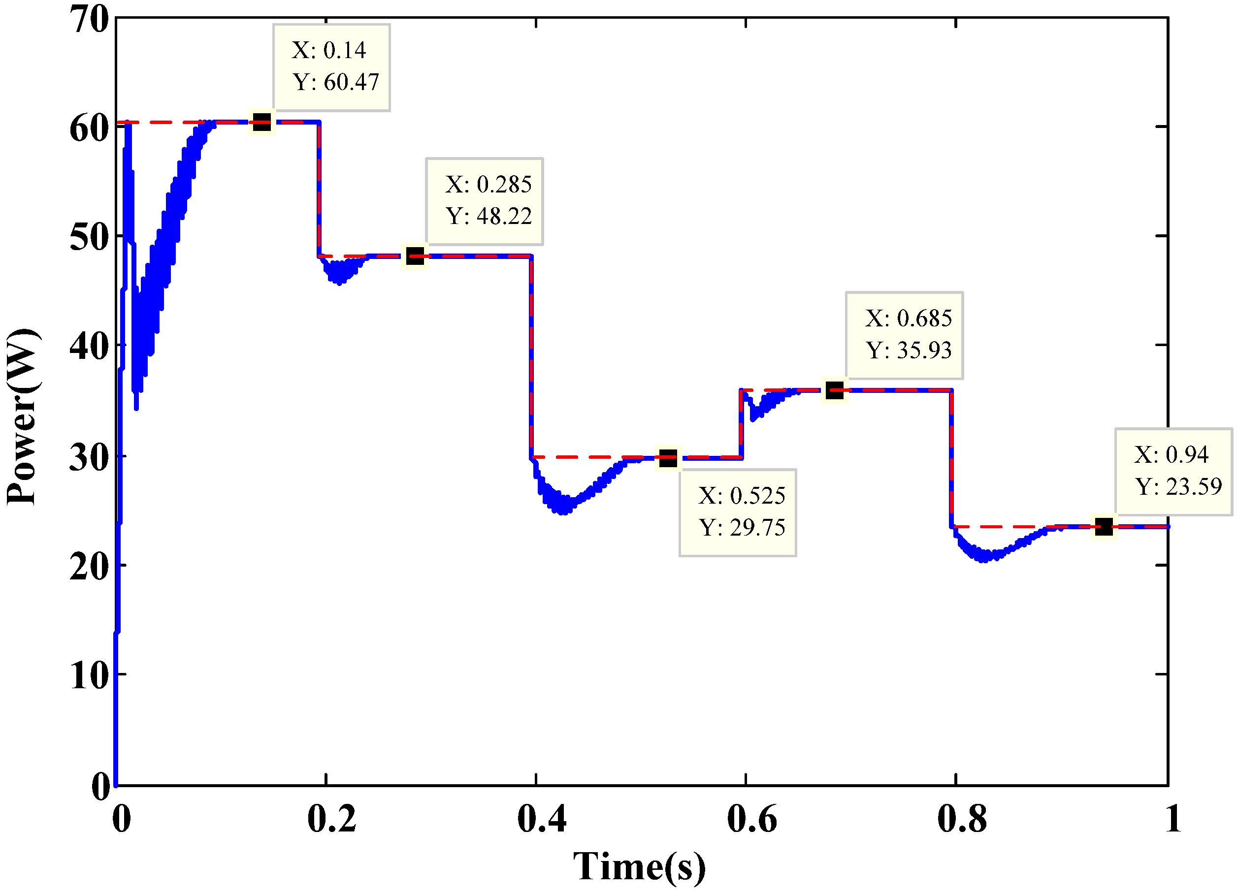
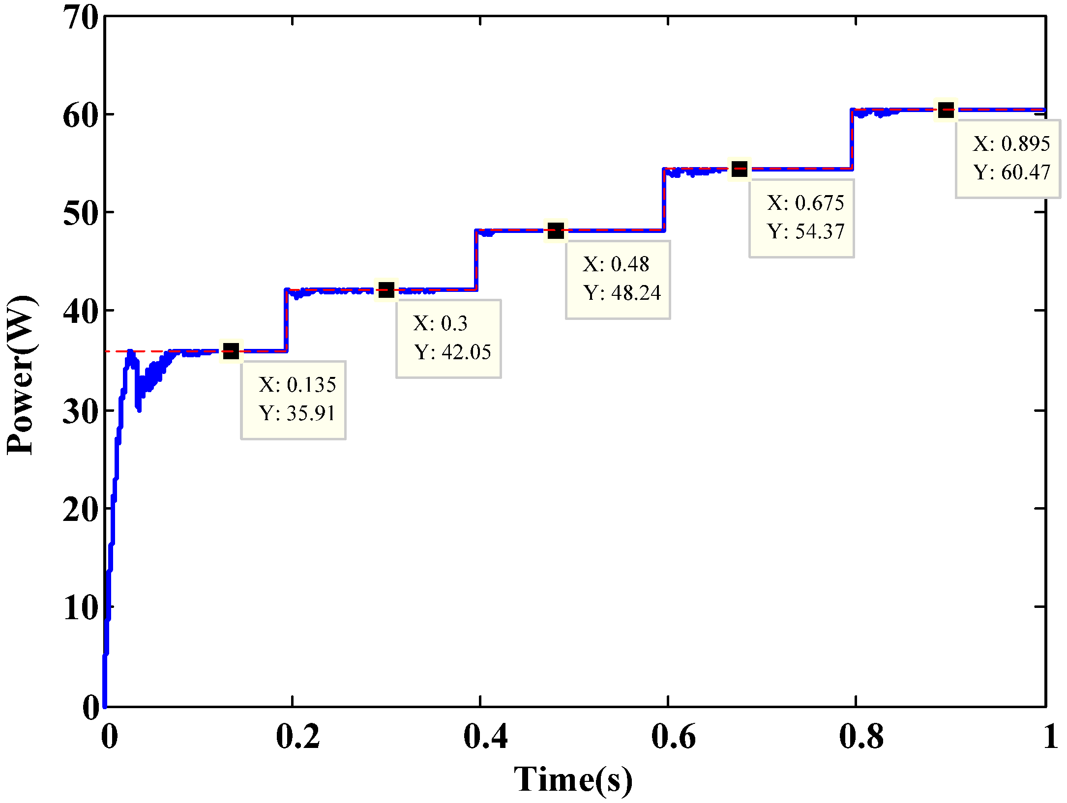
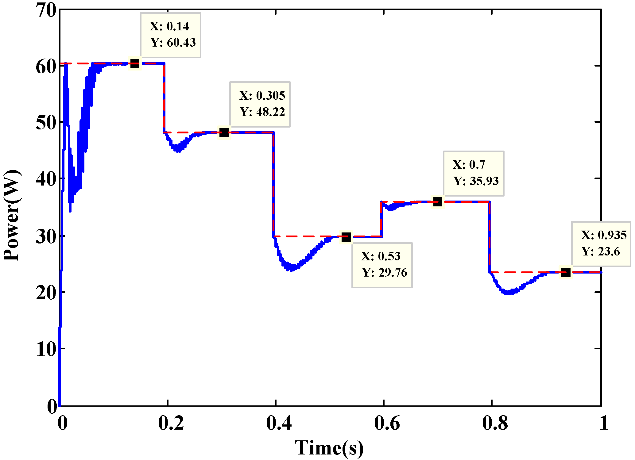
	PV maximum power (W)	60.47	48.25	29.764	35.93	23.60
Algorithm (i)	MPPT reached (W)	60.43	48.22	29.76	35.93	23.60
	Settling time (sec)	0.080	0.050	0.096	0.030	0.097
Algorithm (ii)	MPPT reached (W)	60.47	48.22	29.75	35.93	23.59
	Settling time (sec)	0.085	0.048	0.090	0.039	0.094
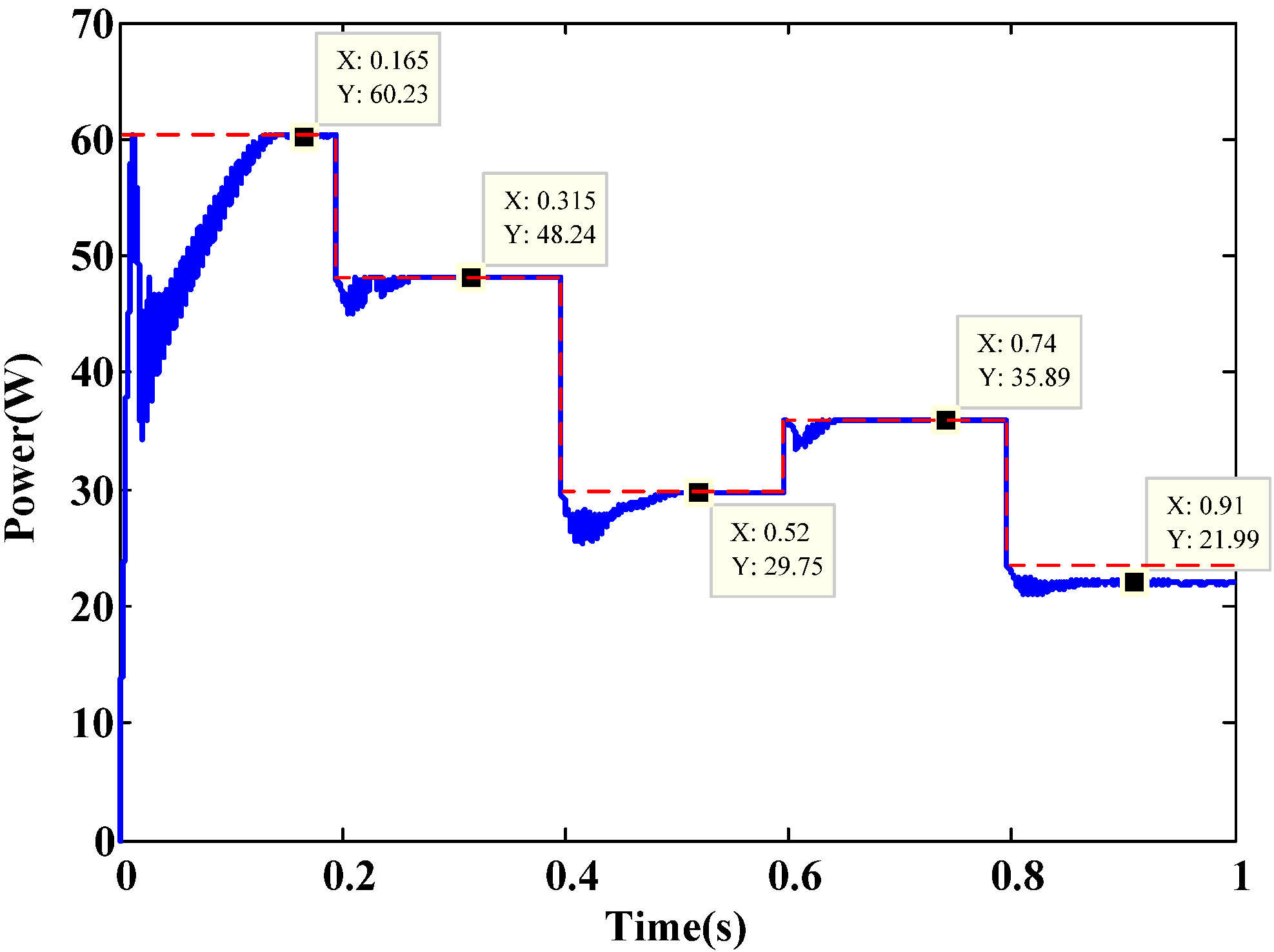
Algorithm (iii)	MPPT reached (W)	60.23	48.24	29.75	35.89	21.99
	Settling time (sec)	0.125	0.050	0.090	0.035	0.052
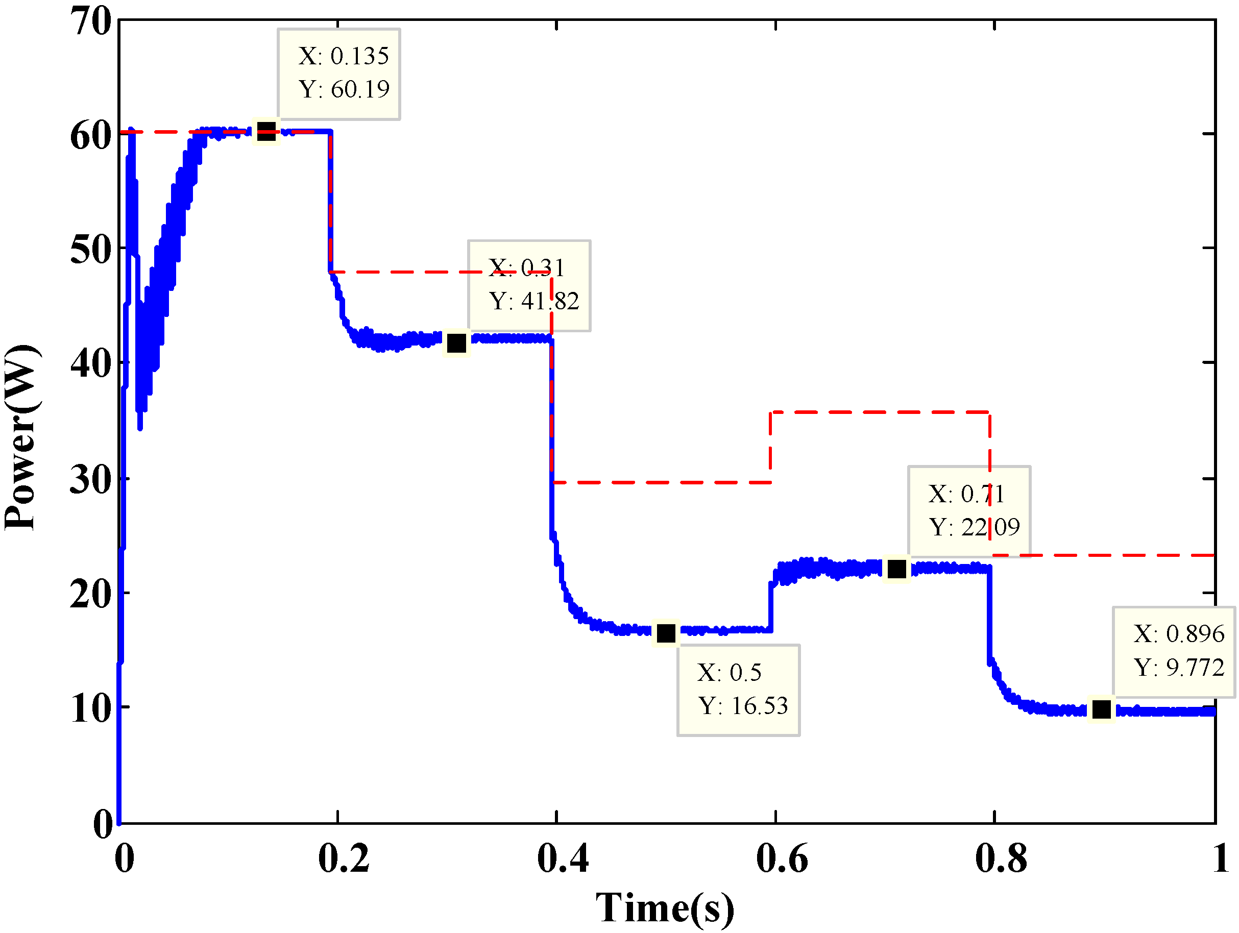
Algorithm (iv)	MPPT reached (W)	60.19	41.88	16.53	22.09	9.77
	Settling time (sec)	0.080	-	-	-	-
Algorithm (v)	MPPT reached (W)	60.41	48.24	29.75	35.86	23.52
	Settling time (sec)	0.060	0.056	0.134	0.030	0.114
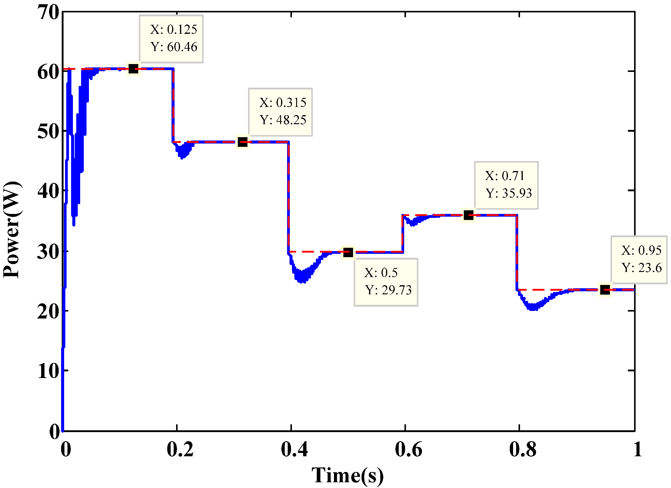
Algorithm (vi)	MPPT reached (W)	60.46	48.25	29.73	35.93	23.60
	Settling time (sec)	0.052	0.030	0.065	0.034	0.084

4. Conclusions

This paper summarized the designs of six fuzzy MPPT algorithms using different input variables. Detailed considerations, determinations of the fuzzy rules associated with the different fuzzy input variables, as well as the advantages and disadvantages of the algorithms have also been summarized in the paper. Algorithm (vi), which used the sum of the angles of the arctangent of the conductance and the arctangent of the incremental conductance as the input variable, was considered the most promising MPPT algorithm according to our considerations as the MPP conditions would have a well-defined range for both the sum (${180}^{\text{o}}$) and the range of the sum (90~270°). When compared to other algorithms, Algorithm (vi) made it easier to determine the range of the universe of discourse, fuzzy rules, and the associated membership functions for the MPPT algorithm. Computer simulation also confirmed that Algorithm (vi) provided better MPPT performance. Additionally, the MPPT function could also be formulated as a form of feedback control using ${180}^{\text{o}}$ as the reference input and be applied in multipurpose controller designs such as by incorporating of voltage regulation purposes.

References

- International Energy Agency. Technology Roadmap: Solar Photovoltaic Energy; IEA Publications: Paris, France, 2014. Available online: http://www.iea.org/publications/freepublications/publication/TechnologyRoadmapSolarPhotovoltaicEnergy_2014edition.pdf (accessed on 10 October 2014).
- Tomabechi, K. Energy Resources in the Future. Energies 2010, 3, 686–695. [Google Scholar] [CrossRef]
- Femia, N.; Petrone, G.; Spagnuolo, G.; Vitellio, M. Optimization of Perturb and Observe Maximum Power Point Tracking Method. IEEE Trans. Power Electron. 2005, 20, 963–973. [Google Scholar] [CrossRef]
- Hussen, K.H.; Muta, I.; Hoshino, T.; Osakada, M. Maximum photovoltaic power tracking: An algorithm for rapidly changing atmospheric conditions. IEE Gener. Transm. Distrib. 1995, 142, 59–64. [Google Scholar] [CrossRef]
- Mohd Zainuri, M.A.A.; Mohd Radzi, M.A.; Soh, A.C.; Abdul Rahim, N. Adaptive P&O-Fuzzy Control MPPT for PV Boost Dc-Dc Converter. In Proceedings of the 2012 IEEE International Conference on Power and Energy (PECon), Kota Kinabalu Sabah, Malaysia, 2–5 December 2012; pp. 524–529.
- Yong, T.; Xia, B.; Xu, Z.; Sun, W. Modified Asymmetrical Variable Step Size Incremental Conductance Maximum Power Point Tracking Method for Photovoltaic Systems. J. Power Electron. 2014, 14, 156–164. [Google Scholar] [CrossRef]
- Alajmi, B.N.; Ahmed, K.H.; Finney, S.J.; Williams, B.W. Fuzzy-Logic-Control Approach of a Modified Hill-Climbing Method for Maximum Power Point in Microgrid Standalone Photovoltaic System. IEEE Trans. Power Electron. 2011, 26, 1022–1030. [Google Scholar] [CrossRef]
- Iqbal, A.; Abu-Rub, H.; Ahmed, S.M. Adaptive Neuro-Fuzzy Inference System based Maximum Power Point Tracking of a Solar PV Module. In Proceedings of the 2010 IEEE International Energy Conference and Exhibition (EnergyCon), Manama, Bahrain, 18–22 December 2010; pp. 51–56.
- Chin, C.S.; Neelakantan, P.; Yoong, H.P.; Teo, K.T.K. Optimisation of Fuzzy based Maximum Power Point Tracking in PV System for Rapidly Changing Solar Irradiance. Trans. Sol. Energy Plan. 2011, 2, 130–137. [Google Scholar]
- Radjai, T.; Gaubert, P.J.; Rahmani, L. The new FLC-Variable Incremental Conductance MPPT Direct Control Method Using Cuk Converter. In Proceedings of the 2014 IEEE 23rd International Symposium on Industrial Electronics (IEIE), Istanbul, Turkey, 1–4 June 2014; pp. 2508–2513.
- Aït Cheikh, M.S.; Larbes, C.; Tchoketch Kebir, G.F.; Zerguerras, A. Maximum power point tracking using a fuzzy logic control scheme. Revue Energ. Renouv. 2007, 10, 387–395. [Google Scholar]
- Rahmani, R. Mohammadmehdi Seyedmahmoudian, Saad Mekhilef and Rubiyah Yusof, Implementation of Fuzzy Logic Maximum Power Point Tracking Controller for Photovoltaic System. Am. J. Appl. Sci. 2013, 10, 209–218. [Google Scholar] [CrossRef]
- Liu, C.-L.; Chen, J.-H.; Liu, Y.-H.; Yang, Z.-Z. An Asymmetrical Fuzzy-Logic-Control-Based MPPT Algorithm for Photovoltaic Systems. Energies 2014, 7, 2177–2193. [Google Scholar] [CrossRef]
- Takun, P.; Kaitwanidvilai, S.; Jettanasen, C. Maximum Power Point Tracking using Fuzzy Logic Control for Photovoltaic Systems. In Proceedings of the International MutiConference of Engineers and Computer Scientists, Hong Kong, China, 16–18 March 2011.
- Putri, R.I.; Wibowo, S.; Taufi, M.; Taufik. Fuzzy Incremental Conductance for Maximum Power Point Tracking in Photovoltaic System. Int. J. Eng. Sci. Innov. Technol. (IJESIT) 2014, 3, 352–359. [Google Scholar]
- Sakly, A.; Ben Smida, M. Adequate Fuzzy Inference Method for MPPT Fuzzy Control of Photovoltaic Systems. In Proceedings of the 2012 International Conference on Future Electrical Power and Energy systems, Lecture Notes in Information Technology; 2012; 9, pp. 457–468. [Google Scholar]
- Mahamudul, H.; Saad, M.; Henk, M.I. Photovoltaic System Modeling with Fuzzy Logic Based Maximum Power Point Tracking Algorithm. Int. J. Photoenergy 2013, 2013, 762946. [Google Scholar]
- Khateb, A.H.E.; Rahim, N.A.; Selvaraj, J. Type-2 Fuzzy Logic Approach of a Maximum Power Point Tracking Employing SEPIC Converter for Photovoltaic System. J. Clean Energy Technol. 2013, 1, 41–44. [Google Scholar] [CrossRef]
- Roy, C.P.; Vijaybhaskar, D.; Maity, T. Modelling of Fuzzy Logic Controller for Variable Step MPPT in Photovoltaic System. Int. J. Res. Eng. Technol. 2013, 2, 426–432. [Google Scholar]
- Natsheh, E.M.; Albarbar, A. Hybrid Power Systems Energy Controller Based on Neural Network and Fuzzy Logic. Smart Grid Renew. Energy 2013, 4, 187–197. [Google Scholar] [CrossRef]
- Bos, M.J.; Abhijith, S.; Aswin, V.; Basil, R.; Dhanesh, R. Fuzzy Logic Controlled PV Powered Buck Converter with MPPT. Int. J. Adv. Res. Electr. Electron. Instrum. Eng. 2014, 3, 9370–9377. [Google Scholar]
- Falin, J. Designing DC/DC converters based on ZETA topology. Analog Appl. J. Texas Instruments Incorporated, 2Q. Texas, USA. 2010, 16–21. [Google Scholar]
© 2015 by the authors; licensee MDPI, Basel, Switzerland. This article is an open access article distributed under the terms and conditions of the Creative Commons Attribution license (http://creativecommons.org/licenses/by/4.0/).
Share and Cite
Shiau, J.-K.; Wei, Y.-C.; Chen, B.-C. A Study on the Fuzzy-Logic-Based Solar Power MPPT Algorithms Using Different Fuzzy Input Variables. Algorithms 2015, 8, 100-127. https://doi.org/10.3390/a8020100
Shiau J-K, Wei Y-C, Chen B-C. A Study on the Fuzzy-Logic-Based Solar Power MPPT Algorithms Using Different Fuzzy Input Variables. Algorithms. 2015; 8(2):100-127. https://doi.org/10.3390/a8020100
Chicago/Turabian StyleShiau, Jaw-Kuen, Yu-Chen Wei, and Bo-Chih Chen. 2015. "A Study on the Fuzzy-Logic-Based Solar Power MPPT Algorithms Using Different Fuzzy Input Variables" Algorithms 8, no. 2: 100-127. https://doi.org/10.3390/a8020100
APA StyleShiau, J.-K., Wei, Y.-C., & Chen, B.-C. (2015). A Study on the Fuzzy-Logic-Based Solar Power MPPT Algorithms Using Different Fuzzy Input Variables. Algorithms, 8(2), 100-127. https://doi.org/10.3390/a8020100