Statistical Properties of Protein-Protein Interfaces

Abstract

The properties of 1172 protein complexes (downloaded from the Protein Data Bank (PDB)) have been studied based on the concept of circular variance as a buriedness indicator and the concept of mutual proximity as a parameter-free definition of contact. The propensities of residues to be in the protein, on the surface or form contact, as well as residue pairs to form contact were calculated. In addition, the concept of circular variance has been used to compare the ruggedness and shape of the contact surface with the overall surface.

1. Introduction

Formation of protein complexes is a ubiquitous biological process. However, knowledge of the structure of individual proteins is rarely sufficient to unequivocally predict the interaction surface of two proteins. This problem manifests itself in the performance of various computational tools designed to predict such complex formation: a large number of predicted structures usually look “reasonable”. Given this conundrum, tools that can help improve the ranking of such set of models for a complex can be of significant help.

The increase of the number of complexes in the protein databank led to statistical analyses. Jones and Thorton [1] compared the solvation potential, residue propensity, hydrophobicity, planarity, protrusion and accessible surface area of the interfaces and the rest of the surface of 48 complexes. Progress in the area has been reviewed by Moreira et al. [2]. Energetic and evolutionary properties of the interfaces were examined by Ma et al. [3]. Newer analyses of protein interaction surfaces were done in [4,5,6]. A tool kit [7] and web servers [8,9] are also available that calculate a series of physical and chemical properties of the interaction sites. The role of conserved residues in interaction surfaces has also been studied [10,11,12]. Databases have been developed with characteristics of the cyrstallographically determined interfaces [13,14,15]. A recent study examined the relationship between binding affinity and interfacial buried surface area [16]. The geometry of interaction surfaces has also been studied [17] using Voronoi tessellation [18]. A method measuring the surface roughness, different from the one described in Section 3.2 has been introduced in [19]. A method differentiating between flat and protruding/interwinding interaction surfaces, different from the one described in Section 3.3 has been described in [20].

The present paper applies the concept of mutual proximity to delineate contact pairs on the interaction surface and uses the concept of the circular variance to examine some geometric properties of the interaction surface.

2. Experimental Section

The calculations presented in this paper are based on a number of geometric concepts introduced previously: accessible surface, circular variance and mutual proximity. Here, they are introduced briefly.

Accessible surface [21] is an extension of the Vander Waals (VdW) surface. It is defined by the center of a solvent-size sphere (in case of water of radius 1.4 Å) as it is rolled around the VdW surfaces of the atoms in the target. Such a surface is generally smoother than the VdW surface as the solvent sphere does not fit into the crevices formed by the VdW surfaces of atoms.

Circular Variance (CV), a concept introduced for the characterization of angular spread [22] has been found to be useful to characterize the extent a point is buried within a set of points [23]. The degree of buriedness indicator is calculated as the circular variance of vectors drawn from a test point to the points in the set: when the test point is way outside then these vectors are essentially parallel, so CV is near zero while when the test point is in the middle of the set then CV will be close to one:

$$CV=1- \frac{|{{\displaystyle \sum }}_i{\overrightarrow{r}}_i-\overrightarrow{R}|}{{{\displaystyle \sum }}_i|{\overrightarrow{r}}_i-\overrightarrow{R}|}$$

where {${\overrightarrow{r}}_i$} is the set vectors pointing to the atoms of the protein and $\overrightarrow{R}$ is the vector pointing to the test point.

The concept of mutual proximity was used earlier to establish the contacts between a target and a docked ligand pose[24]. In this application, for each atom in a pair of proteins the one nearest to it from the other protein is established; whenever atom i₁ is nearest to i₂ and at the same time atom i₂ is nearest to i₁ the pair of atoms [i₁, i₂] is considered a contact pair. Figure 1 shows a schematic demonstrating the relation between contact and mutual proximity.

It was also found that a robust definition of surface atoms is obtained if atoms whose exposed accessible surface fraction exceeds 3% and whose CV calculated with respect to the rest of the protein atoms is less than 0.8 are selected. As the average distance between closest pair contact atoms is 5.0 Å surface atoms within 4 Å were considered part of the interface. This choice ensured that most, if not all, non-contact surface atoms were included in the interface. All statistics reported in this paper were calculated using these definitions. As the data involved crystal structures, only heavy atoms were considered.

The test data set contained 1172 protein complexes, downloaded from the Protein Data Bank (PDB) [25]. The complexes selected were of high resolution and had no missing residues. For each complex, the PDB annotation for biological oligomers was used. When the complex contained more than two members, the pair with the largest number of contacts was retained. The PDB IDs of the 1172 complexes, together with the chain IDs used is provided as supporting information.

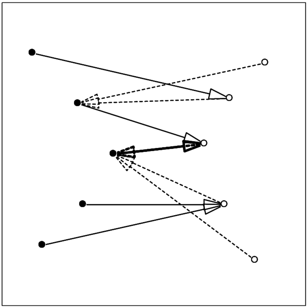
Figure 1. Schematic showing the relation between mutual proximity and contact. Arrows from one component (filled circles, full line) to the other component (open circles) show the nearest atom in the other set; arrows with broken line show the nearest atom in the first set. The two-headed thick arrow shows the mutually proximal pair.

Figure 1. Schematic showing the relation between mutual proximity and contact. Arrows from one component (filled circles, full line) to the other component (open circles) show the nearest atom in the other set; arrows with broken line show the nearest atom in the first set. The two-headed thick arrow shows the mutually proximal pair.

3. Results and Discussion

3.1. Residue Propensities

Based on our definition of surface and contact atoms, the number of occurrence of each of the 20 amino acids (AA) were calculated in the whole set, the set of surface atoms and the set of contact atoms. The results are in Table 1, with AAs arranged in the order of hydrophobic, polar, charged. Columns 1, 2, and 4 of Table 1 show the percent of time each residue occurred in the dataset (all), on the surface (surf) or among the contact atoms (cont), resp. Note that uniformly distributed residues would all show up with 5%. Column 3 shows the ratio of surface and overall propensities; not surprisingly the excess likelihood of being on the surface increases moving from the hydrophobic to the charged residues. Residues participating in multiple contacts were only counted once.

Table 1. Residue propensities to appear (all), be on the surface (surf) or form contact (cont).

	%(all)	%(surf)	%(surf)/%(all)	%(cont)	%(cont)/%(all)	%(cont)/%(surf)
GLY	6.97	6.32	0.91	5.27	0.76	0.83
ALA	6.83	5.42	0.79	4.55	0.67	0.84
VAL	6.80	5.03	0.74	5.23	0.77	1.04
LEU	8.72	6.45	0.74	6.47	0.74	1.00
ILE	5.33	3.96	0.74	4.79	0.90	1.21
PHE	3.70	2.89	0.78	4.24	1.15	1.47
TRP	2.10	2.11	1.00	2.98	1.42	1.41
TYR	4.07	4.31	1.06	6.23	1.53	1.44
PRO	5.08	5.62	1.11	5.50	1.08	0.98
MET	1.81	1.58	0.87	2.22	1.22	1.40
SER	5.88	6.19	1.05	5.17	0.88	0.83
THR	6.13	6.51	1.06	5.58	0.91	0.86
CYS	1.83	1.13	0.62	1.58	0.86	1.39
ASN	4.21	4.86	1.16	5.09	1.21	1.05
HIS	2.39	2.68	1.12	3.60	1.50	1.34
GLN	4.62	5.62	1.22	6.02	1.30	1.07
ASP	5.53	6.65	1.20	6.11	1.10	0.92
GLU	6.81	8.44	1.24	6.15	0.90	0.73
LYS	6.43	8.25	1.28	5.87	0.91	0.71
ARG	4.76	5.97	1.25	7.36	1.55	1.23

Table 1. Residue propensities to appear (all), be on the surface (surf) or form contact (cont).

	%(all)	%(surf)	%(surf)/%(all)	%(cont)	%(cont)/%(all)	%(cont)/%(surf)
GLY	6.97	6.32	0.91	5.27	0.76	0.83
ALA	6.83	5.42	0.79	4.55	0.67	0.84
VAL	6.80	5.03	0.74	5.23	0.77	1.04
LEU	8.72	6.45	0.74	6.47	0.74	1.00
ILE	5.33	3.96	0.74	4.79	0.90	1.21
PHE	3.70	2.89	0.78	4.24	1.15	1.47
TRP	2.10	2.11	1.00	2.98	1.42	1.41
TYR	4.07	4.31	1.06	6.23	1.53	1.44
PRO	5.08	5.62	1.11	5.50	1.08	0.98
MET	1.81	1.58	0.87	2.22	1.22	1.40
SER	5.88	6.19	1.05	5.17	0.88	0.83
THR	6.13	6.51	1.06	5.58	0.91	0.86
CYS	1.83	1.13	0.62	1.58	0.86	1.39
ASN	4.21	4.86	1.16	5.09	1.21	1.05
HIS	2.39	2.68	1.12	3.60	1.50	1.34
GLN	4.62	5.62	1.22	6.02	1.30	1.07
ASP	5.53	6.65	1.20	6.11	1.10	0.92
GLU	6.81	8.44	1.24	6.15	0.90	0.73
LYS	6.43	8.25	1.28	5.87	0.91	0.71
ARG	4.76	5.97	1.25	7.36	1.55	1.23

Columns 5 and 6 of Table 1 show the ratios %(cont)/%(all) and %(cont)/%(surf), resp. It is the last column that gives the most striking result: there are significant differences between the contact forming propensities of surface residues. All three aromatic AAs are strong contact formers but so are MET, CYS and HIS. Interestingly, of the charged residues only ARG shows significant contact forming propensity. Recent work showed that “hot spots” of protein-protein interactions frequently contain tryptophan, arginine, and tyrosine—this is in accordance with their larger contact-forming propensities found in the present study [26].

Table 2 shows the contact-pair forming propensities of AA pairs. The table values are normalized by the surface propensities of the contributing residues:

$$P{R}_{i,j}=\frac{N_{i,j}}{{{\displaystyle \sum }}_{i,j=1}^{20}{N}_{i,j}}/[P_i*P_i*\left(2-{\text{δ}}_{i,j}\right)]$$

where PR_i,j is the propensity of the residue pair {i, j} to form contact, P_i is the probability of residue i being on the surface, N_i,j is the number of {i, j} pairs found in the data set and δ_i,j is the Kronecker delta (one when i = j, zero otherwise). This means that if a residue does not have any preference for contacting residues then the entries involving that residue should be all ones. PR_i,j values over 3.0 are highlighted in bold type.

Table 2. Contact pair propensities normalized by surface propensities.

	GLY	ALA	VAL	LEU	ILE	PHE	TRP	TYR	PRO	MET	SER	THR	CYS	ASN	HIS	GLN	ASP	GLU	LYS	ARG
GLY	0.65
ALA	0.31	0.70
VAL	0.59	0.52	1.36
LEU	0.59	0.81	1.46	1.29
ILE	0.68	0.99	1.09	2.60	2.30
PHE	0.77	1.68	1.73	2.51	2.99	10.0
TRP	1.19	1.99	1.78	1.73	1.23	3.24	9.12
TYR	1.00	1.03	1.56	1.59	2.35	3.54	2.75	3.23
PRO	1.04	0.73	1.01	1.24	0.87	1.85	2.69	2.17	0.61
MET	0.61	0.54	1.17	1.64	1.28	3.80	7.40	3.41	0.99	3.68
SER	0.46	0.45	0.89	0.45	0.39	1.36	0.95	0.87	0.79	0.93	0.58
THR	0.55	0.65	0.90	0.68	0.88	1.82	1.70	1.50	0.64	1.10	0.41	0.62
CYS	1.55	0.92	1.09	1.60	1.25	1.31	2.25	1.05	0.45	0.75	0.35	0.34	17.2
ASN	0.77	1.42	0.73	0.84	1.22	1.39	4.28	1.23	1.18	0.79	0.68	0.77	1.56	1.02
HIS	2.07	0.46	1.12	0.69	1.52	1.81	2.92	3.20	0.40	1.56	0.77	0.99	2.30	1.37	2.78
GLN	0.68	0.47	1.20	0.80	1.00	1.46	4.37	1.48	1.07	1.25	0.56	1.07	0.91	0.65	1.89	1.17
ASP	0.30	0.47	0.64	0.37	0.94	0.90	2.21	1.19	0.64	0.96	0.82	0.60	0.17	0.76	2.30	0.63	0.31
GLU	0.37	0.21	0.85	0.39	0.70	0.84	0.64	1.37	0.54	0.62	0.77	0.46	0.47	0.62	1.32	1.46	0.31	0.21
LYS	0.38	0.32	0.45	0.41	0.71	0.96	1.00	1.37	0.26	0.79	0.50	0.53	0.92	0.71	0.52	0.49	1.12	1.16	0.47
ARG	1.23	0.92	1.04	0.76	1.13	2.56	3.05	3.44	0.63	3.65	0.81	0.86	1.54	1.35	1.32	1.91	2.88	1.67	0.58	0.86
	GLY	ALA	VAL	LEU	ILE	PHE	TRP	TYR	PRO	MET	SER	THR	CYS	ASN	HIS	GLN	ASP	GLU	LYS	ARG

Table 2. Contact pair propensities normalized by surface propensities.

	GLY	ALA	VAL	LEU	ILE	PHE	TRP	TYR	PRO	MET	SER	THR	CYS	ASN	HIS	GLN	ASP	GLU	LYS	ARG
GLY	0.65
ALA	0.31	0.70
VAL	0.59	0.52	1.36
LEU	0.59	0.81	1.46	1.29
ILE	0.68	0.99	1.09	2.60	2.30
PHE	0.77	1.68	1.73	2.51	2.99	10.0
TRP	1.19	1.99	1.78	1.73	1.23	3.24	9.12
TYR	1.00	1.03	1.56	1.59	2.35	3.54	2.75	3.23
PRO	1.04	0.73	1.01	1.24	0.87	1.85	2.69	2.17	0.61
MET	0.61	0.54	1.17	1.64	1.28	3.80	7.40	3.41	0.99	3.68
SER	0.46	0.45	0.89	0.45	0.39	1.36	0.95	0.87	0.79	0.93	0.58
THR	0.55	0.65	0.90	0.68	0.88	1.82	1.70	1.50	0.64	1.10	0.41	0.62
CYS	1.55	0.92	1.09	1.60	1.25	1.31	2.25	1.05	0.45	0.75	0.35	0.34	17.2
ASN	0.77	1.42	0.73	0.84	1.22	1.39	4.28	1.23	1.18	0.79	0.68	0.77	1.56	1.02
HIS	2.07	0.46	1.12	0.69	1.52	1.81	2.92	3.20	0.40	1.56	0.77	0.99	2.30	1.37	2.78
GLN	0.68	0.47	1.20	0.80	1.00	1.46	4.37	1.48	1.07	1.25	0.56	1.07	0.91	0.65	1.89	1.17
ASP	0.30	0.47	0.64	0.37	0.94	0.90	2.21	1.19	0.64	0.96	0.82	0.60	0.17	0.76	2.30	0.63	0.31
GLU	0.37	0.21	0.85	0.39	0.70	0.84	0.64	1.37	0.54	0.62	0.77	0.46	0.47	0.62	1.32	1.46	0.31	0.21
LYS	0.38	0.32	0.45	0.41	0.71	0.96	1.00	1.37	0.26	0.79	0.50	0.53	0.92	0.71	0.52	0.49	1.12	1.16	0.47
ARG	1.23	0.92	1.04	0.76	1.13	2.56	3.05	3.44	0.63	3.65	0.81	0.86	1.54	1.35	1.32	1.91	2.88	1.67	0.58	0.86
	GLY	ALA	VAL	LEU	ILE	PHE	TRP	TYR	PRO	MET	SER	THR	CYS	ASN	HIS	GLN	ASP	GLU	LYS	ARG

3.2. Ruggedness of the Interaction Surface

The calculated CV value can also be used to characterize the smoothness or ruggedness of region of the molecular surface. In a smooth surface the difference between the CV values of neighboring surface atoms is small; the more rugged the surface, the larger the CV differences are. This suggests a ruggedness indicator at a surface atom i, RG(i):

$$G\left(i\right)={\displaystyle \sum }_{\text{{}k\text{|} \left|\overrightarrow{r_k}-\overrightarrow{ r_i}\right|< R_N\}}\frac{\left|CV\left(i\right)-CV\left(k\right)\right|}{N_n(i)}$$

where $\overrightarrow{r_k}$ is a surface neighbor atom of i and N_n(i) is the number of surface neighbors of atom i. To differentiate the interaction surface from the overall surface atoms that are within 4 Å of a contact atom are considered to be part of the interaction surface.

The average number of surface atoms, contact atoms, interaction surface atoms were found to be 307.0, 50.8, 72.8, resp. The average RG values of the interaction and full surface atoms were found to be 0.069 (s.d. = 0.007) and 0.066 (s.d. = 0.005), resp. The difference is significant at the level p = 0.001. Thus it can be concluded that interaction surfaces are more rugged than the rest.

3.3. Shape of the Interaction Surface

Comparison of the average CV values of different surface regions can also tell if a particular surface area is protruding or is recessed: The average CV value of a protruding surface area is smaller than the overall average of the surface atoms’ CV value, while the recessed region’s CV average is larger.

Using the definition of interaction surface as above, the CV values of the interaction and full surface were found to be 0.454 (s.d. = 0.044) and 0.464 (s.d. = 0.029), resp. While this difference is quite small it is significant at the level p = 0.001 according to the Student t test. Thus, we can conclude that the interaction surface is likely to be protruding, even if only slightly.

4. Conclusions

Use of the parameter-free definition of contact and the concept of circular variance as a buriedness indicator, several properties of protein-protein interfaces were found to be different from those of the overall surface. It is expected that these properties can be exploited as additional filter, aiding in selecting the best model from the result of in silico predictions.

Identification of residues with high propensity for contact forming can also aid drug discovery. Significant numbers of drugs are designed to disrupt protein-protein associations and thus targeting residues that are more likely to form contacts increases the probability of success when searching for lead compounds.

The data set used for these comparisons has not been filtered for size or strength of interaction or the size of the interface. It is quite possible that partitioning the data set can refine these differences found: for some subsets the differences could be larger, for others they may become insignificant. Furthermore, some of the results presented are based on a specific definition of contact surface—other definitions may change the results.

References

- Jones, J.; Thorton, J.M. Analysis of protein-protein interaction sites using surface patches. J. Mol. Biol. 1997, 272, 121–132. [Google Scholar] [CrossRef] [PubMed]
- Moreira, I.S.; Fernandes, P.A.; Ramos, M.J. Hot spots—A review of the protein-protein interface determinant amino-acid residues. Proteins 2007, 68, 803–812. [Google Scholar] [CrossRef] [PubMed]
- Ma, B.; Elkayam, T.; Wolfson, H.; Nussinov, R. Protein-protein interactions: Structurally conserved residues distinguish between binding sites and exposed protein surfaces. Proc. Natl. Acad. Sci. USA 2003, 100, 5772–5777. [Google Scholar] [CrossRef] [PubMed]
- Yan, C.; Wu, F.; Jernigan, R.L.; Dobbs, D.; Honavar, V. Characterization of protein-protein interfaces. Protein J. 2008, 27, 59–70. [Google Scholar] [CrossRef] [PubMed]
- Hu, J.; Yan, C. A comparative analysis of protein interfaces. Protein Pept. Lett. 2010, 17, 1450–1458. [Google Scholar] [CrossRef] [PubMed]
- Kysilka, J.; Vondrášek, J. Towards a better understanding of the specificity of protein-protein interaction. J. Mol. Recognit. 2012, 25, 604–615. [Google Scholar] [CrossRef] [PubMed]
- Gruber, J.; Zawaira, A.; Saunders, R.; Barrett, C.P.; Noble, M.E. Computational analyses of the surface properties of protein-protein interfaces. Acta Crystallogr. Sect. D Biol. Crystallogr. 2007, 63, 50–57. [Google Scholar] [CrossRef]
- Reynolds, C.; Damerell, D.; Jones, S. Protorp: A protein-protein interaction analysis server. Bioinformatics 2009, 25, 413–414. [Google Scholar] [CrossRef] [PubMed]
- Vangone, A.; Spinelli, R.; Scarano, V.; Cavallo, L.; Oliva, R. Cocomaps: A web application to analyze and visualize contacts at the interface of biomolecular complexes. Bioinformatics 2011, 27, 2915–2916. [Google Scholar] [CrossRef] [PubMed]
- Guharoy, M.; Chakrabarti, P. Conserved residue clusters at protein-protein interfaces and their use in binding site identification. BMC Bioinform. 2010, 11, 286. [Google Scholar] [CrossRef]
- Eichborn, J.V.; Günther, S.; Preissner, R. Structural features and evolution of protein-protein interactions. Genome Inform. 2010, 22, 1–10. [Google Scholar] [PubMed]
- Duarte, J.M.; Srebniak, A.; Schärer, M.A.; Capitani, G. Protein interface classification by evolutionary analysis. BMC Bioinform. 2912, 13, 334. [Google Scholar] [CrossRef]
- Baskaran, K.; Duarte, J.M.; Biyani, N.; Bliven, S.; Capitani, G. A pdb-wide, evolution-based assessment of protein-protein interfaces. BMC Struct. Biol. 2014. [Google Scholar] [CrossRef]
- Teyra, J.; Doms, A.; Schroeder, M.; Pisabarro, M. Scowlp: A web-based database for detailed characterization and visualization of protein interfaces. BMC Bioinform. 2006, 7, 104. [Google Scholar] [CrossRef]
- Kundrotas, P.; Zhu, Z.; Vakser, I.A. Gwidd: Genome-wide protein docking database. Nucleic Acids Res. 2010, 38, D513–D517. [Google Scholar] [CrossRef] [PubMed]
- Chen, J.; Sawyer, N.; Regan, L. Protein-protein interactions: General trends in the relationship between binding affinity and interfacial buried surface area. Protein Sci. 2013, 22, 510–515. [Google Scholar] [CrossRef] [PubMed]
- Mahdavia, S.; Salehzadeh-Yazdia, A.; Mohadesb, A.; Masoudi-Nejad, A. Computational structure analysis of biomacromolecule complexes by interface geometry. Comput. Biol. Chem. 2013, 47, 16–23. [Google Scholar] [CrossRef] [PubMed]
- Voronoi, G. Nouvelles applications des paramètres continus à la théorie des formes quadratiques. Journal für die reine und angewandte Mathematik 1908, 1908, 97–102. [Google Scholar]
- Bera, I.; Ray, S. A study of interface roughness of heteromeric obligate and non-obligate protein-protein complexes. Bioinformation 2009, 4, 210–215. [Google Scholar] [CrossRef] [PubMed]
- Yura, K.; Hayward, S. The interwinding nature of protein-protein interfaces and its implication for protein complex formation. Bioinformatics 2009, 25, 3108–3113. [Google Scholar] [CrossRef] [PubMed]
- Lee, B.; Richards, F.M. The interpretation of protein structures: Estimation of static accessibility. J. Mol. Biol. 1971, 55, 379–400. [Google Scholar] [CrossRef] [PubMed]
- Mardia, K.V.; Jupp, P.E. Directional Statistics; John Wiley & Sons, Ltd: Chichester, UK, 2000. [Google Scholar]
- Mezei, M. A new method for mapping macromolecular topography. J. Mol. Graph. Model. 2003, 21, 463–472. [Google Scholar] [CrossRef] [PubMed]
- Mezei, M.; Zhou, M.M. Dockres: A computer program that analyzes the output of virtual screening of small molecules. Source Code Biol. Med. 2010, 5, 2. [Google Scholar] [CrossRef] [PubMed]
- Berman, H.M.; Westbrook, J.; Feng, Z.; Gilliland, G.; Bhat, T.N.; Weissig, H.; Shindyalov, I.N.; Bourne, P.E. The protein data bank. Nucleic Acids Res. 2000, 28, 235–242. [Google Scholar] [CrossRef] [PubMed]
- Falchi, F.; Caporuscio, F.; Recanatini, M. Structure-based design of small-molecule protein–protein interaction modulators: The story so far. Future Med. Chem. 2014, 6, 343–357. [Google Scholar] [CrossRef] [PubMed]
© 2015 by the author; licensee MDPI, Basel, Switzerland. This article is an open access article distributed under the terms and conditions of the Creative Commons Attribution license (http://creativecommons.org/licenses/by/4.0/).