Article

Power Cable Fault Recognition Based on an Annealed Chaotic Competitive Learning Network

1
College of Electrical and Control Engineering, Xi'an University of Science and Technology, Xi'an 710054, China
2
Department of Computer Science & Information Engineering, National Chin-Yi University of Technology, Taichung 41170, Taiwan
*
Author to whom correspondence should be addressed.
Algorithms 2014, 7(4), 492-509; https://doi.org/10.3390/a7040492
Submission received: 13 June 2014 / Revised: 3 September 2014 / Accepted: 15 September 2014 / Published: 26 September 2014
(This article belongs to the Special Issue Advanced Data Processing Algorithms in Engineering)

Abstract

:
In electric power systems, power cable operation under normal conditions is very important. Various cable faults will happen in practical applications. Recognizing the cable faults correctly and in a timely manner is crucial. In this paper we propose a method that an annealed chaotic competitive learning network recognizes power cable types. The result shows a good performance using the support vector machine (SVM) and improved Particle Swarm Optimization (IPSO)-SVM method. The experimental result shows that the fault recognition accuracy reached was 96.2%, using 54 data samples. The network training time is about 0.032 second. The method can achieve cable fault classification effectively.

1. Introduction

With the rapid development of social economy, and the improvement of science and technology, people rely on power more intensely, and the demand for power resources continues to expand, for which China’s power industry has entered a phase of vigorous development. With the rapid development of urban areas, urban land-value rises year after year and electric underground cables have increased year by year. The demands for the use of electric underground cables under the condition of market economy are increasing. With the development of the energy industry, all kinds of cables are, increasingly, used in various fields of production and life. Power cables not only convey the transmission of information, but are also an important part of manufacturing electrical equipment and instrumentation. In the future, power cable will bring us to an information-based society. Cables buried underground have the advantages of safety and reliability, and small influence due to climate, compared with the overhead lines. However, a power cable will cause different kinds of fault due to long-term use, increase of load, etc. The power cables buried underground are invisible and once a fault happens, the fault is very difficult to find; it often takes several hours, or more, to find a fault. Therefore, not only will this cause a waste of manpower and material resources, but will also cause huge economic losses, such as the production accidents, the banking system, airport scheduling systems, or rail transport systems. It will bring a great deal of inconvenience to our daily lives.
With the gradual development of production technology, in terms of the infrastructure of power systems, the circuit of electrical cables becomes more complex. In the power system, the cable fault needs to be removed the first time, but also must meet the selectivity of relay protection and be reliable, in addition to the type of the fault recognition, in order to repair the cable fault as soon as possible. Thus, the fault signal feature extraction and cable fault analysis are very important for the correct action for relay protection and different kinds of fault-type recognition, and the safety of the power system [1]. Once the power cable fault occurs, the fault is very difficult to find. With the increase of various cable faults, it causes great economic losses, directly or indirectly. Detecting the fault location of power cables accurately, and recognizing the fault type quickly, are important tasks in a normal power system. Generally, cable faults can be caused by the following several cases: ageing of insulation, heat load, mechanical damage, corrosion protection layer, overvoltage, material defects, etc. We focus on the research of fault-type recognition in this paper.
Cable fault type recognition has been researched widely. There are different kinds of fault recognition methods, such as wavelet analysis, artificial neural network, particle swarm optimization (PSO) [2,3,4], support vector machine (SVM) [5,6,7], the improved PSO-SVM algorithm, etc. The transient traveling wave signal of the cable fault is disposed of by the wavelet transformation, based on cable traveling wave transmission theory [8,9,10]. Electric-heating cable fault testing is based on a neural network [11]. An improved particle swarm optimization and support vector machine recognize the power cable fault types [12]. An adaptive procedure for the problem of synchronization and parameter identification for chaotic networks is proposed [13].
An annealed chaotic competitive network, recognizing power cable fault types is proposed in this paper. Artificial neural networks change their internal structure and form self-adaptive systems in practical applications. They are applied to learning and classification in many different fields. A competitive learning network solves the problem of color image segmentations [14]. A two-layer annealed chaotic competitive learning network detects the image edge [15,16]. Hybrid Hopfield neural networks and a self-adaptive genetic algorithm calibrate camera parameters [17,18]. Fuzzy possibilistic c-means embed into the Hopfield network to construct a classification system [19]. The neural network is classified by the method of clustering in many different fields. In the paper, the method of clustering deals with power cable fault recognition. The chaotic behavior is controlled to escape from local minima by the annealed chaotic competitive learning network. The network architecture classifies the training sample data to generate feasible clusters in clustering problems. A simulated annealing technique having a non-zero probability to go from one state to another, moves toward a bad state temporarily, so as to jump out of local minima. The annealing strategy is added to control the chaotic behavior. The neuron state is refined to reach global optimal results when the energy function is converged. The sample data can be converged effectively in a test and the experiment shows a good performance.
The rest of this paper is organized as follows. First, in Section 2, the competitive learning network and annealed chaotic function are introduced. In Section 3, an annealed chaotic competitive learning network is presented. In Section 4, the network is applied to recognize power cable fault types, and show the experiment. Finally, we conclude in the last section.

2. Related Research

2.1. SupportVector Machine

A Support Vector Machine (SVM) [20] is applied to classify data by finding the best hyperplane that separates all data points of one class from those of another class. Here, the best hyperplane of the SVM means the one with the largest margin between the two classes. Margin means the maximal width of the hyperplane that has no interior data points.
The support vectors are the data points on the boundary of the slab that are closest to the separating hyperplane.
The training data is classified correctly by a given hyperplane. The hyperplane, represented by (w,b), is equally expressed by all pairs { λ w , λ b } for λ R + . Thus, we define the canonical hyperplane to be that which separates the data from the hyperplane by a “distance” of at least 1. That is to say, the relationship satisfies the following formula:
{ x i Τ w + b + 1 , x i Τ w + b 1 , y i = + 1 , y i = 1 , i = 1 , 2 , , l
or, more compactly, as follows:
y i ( x i Τ w + b ) 1 0 , i
Based on the considerations presented above, the optimum separation hyperplane conditions from Equation (2) can be formulated into the following expression that represents a linear SVM:
{ min 1 2 w 2 s . t . y i ( x i Τ w + b ) 1 0 , i
The optimization problem from Equation (3) represents the minimization of a quadratic function under linear constraints. The training data are converted into a feature space with kernel function, and different kernel function cause different effect of classification, thus, the kernel functions in SVM are important for the choice.
Here, the Gaussian RBF kernel is used as follows:
K ( x i , x j ) = exp ( x j x i 2 / ( 2 σ 2 ) )
Width coefficient penalty factor C and radial basis kernel factor σ need to be determined before support vector machine model corresponding to the classification. The parameters of SVM are optimized by the particle swarm optimization algorithm in improved Particle Swarm Optimization-Support Vector machine(IPSO-SVM) method.

2.2. Particle Swarm Optimization Algorithm (PSO)

PSO [21,22,23] is a populated search method, which is used to select c and σ parameters in SVM. It is similar to genetic algorithms. PSO is performed by a population (called swarm) of individuals (called particles) that are updated from iteration to iteration [24,25]. The particle of improved PSO-SVM is composed of two parts, c and σ . To discover the optimal solution, each particle moves in the direction of its previously best position (pbest) and its best global position (gbest). For each particle, i, and dimension, j, search space, assume: particle vector x i = ( x i 1 , x i 2 , ... x i j ) T denotes the current position of the ith particle, the velocity vector v i = ( v i 1 , v i 2 , ... v i j ) T denotes the fly velocity of the ith particle, the velocity and position of particles can be updated by the following equations:
v i j t + 1 = w v i j t + c 1 r 1 ( p i d x i j t ) + c 2 r 2 ( p g d x i j t )
x i j t + 1 = x i j t + v i j t + 1
In the above formula, t is the evolutionary time. v i j is the velocity of particle i on dimension j, of which the value is limited to the range ( v max , v max ), v max value is very important for the algorithm. x i j is the position of particle i on dimension j, of which the value is limited to the range ( x max , x max ). The inertia weight w is used to balance the global exploration and local exploitation. The r 1 and r 2 are random function in the range (0, 1), positive constants c 1 and c 2 are personal and social learning factors.
The method has a great effect on the size of the search space, it is easy to cause the particles to miss the optimal solution if this value is set too large; however, if too small, it can also cause an incomplete search process.
Figure 1 shows velocity and position adjustment of particle at time t0 and t0 + 1. The global optimal solution is at . v 1 indicates flight velocity of “self-awareness” particle toward p b e s t direction at time t0. v 2 indicates flight velocity of “social-consensus” particle toward g b e s t direction at time t0 + 1. v 3 represents the particle’s own current velocity. The particle reaches new particle position x t + 1 at a speed of v t + 1 by the three velocities. Velocity and position of the particle are an iteration process by the method. Finally, the particle constantly keeps close to the optimal position.

2.3. Improved Particle Swarm Optimization-Support Vector Machine (IPSO-SVM) Method

Width coefficient penalty factor C and radial basis kernel factor σ of Support Vector Machine are optimized by Particle Swarm Optimization. The outline of the IPSO-SVM algorithm is given as follows.
Step 1: Initialization. Assume: the size of particle swarm is N, the inertia weight is w, acceleration constant is c 1 , c 2 , maximum number of iterations is t max , set width coefficient penalty factor C and radial basis kernel factor σ , set the position of each particle with p b e s t , the best position of all the particles are expressed by g b e s t .
Step 2: Evaluation of particle. Set the training data of cable as the input data of SVM, establish SVM classification model, then evaluate each particle according to the fitness function.
Step 3: Reset speed and position of each particle.
Step 4: Termination condition. If the maximum number of iterations reaches to the initialization settings or the position of the particle can be stable within a small range, then the iteration will stop. In this process, establish the classification of support vector machine according to the parameters c , σ , otherwise it returns step 2.
Step 5: The test sample data of cable regards as the input data of SVM model, determine the different cable fault type according to output result.
Figure 1. Velocity and position adjustment of particle at time t0 (a) and t0 + 1 (b).
Algorithms 07 00492 g001

2.4. Competitive Learning Network

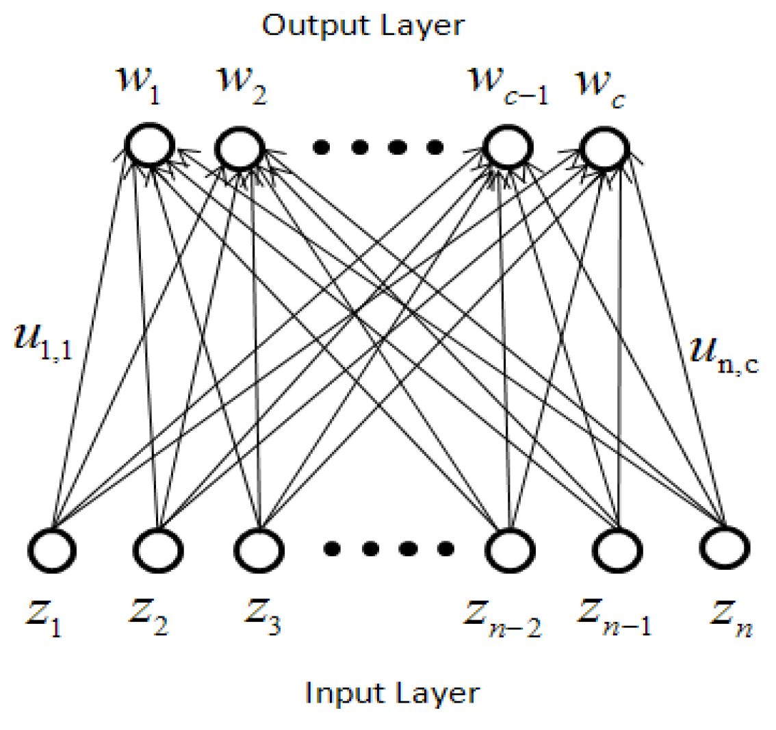
The conventional competitive learning neural network consists of two layers: the input layer, which represents the feature vector, and the output layer, representing the different classification. The network deals with color image segmentation to detect edges and extract boundaries in [16]. The detected different image blocks are classified by the competitive learning network. Different power cable fault types are classified by the method of clustering. Each unit of the network output layer, w j , is fully connected to each unit of the network input layer, z x , with connections u x , j . The topology of the competitive learning network is shown in Figure 2.
Figure 2. The competitive learning neural network topology.
Algorithms 07 00492 g002
The objective function for the network satisfies the following inequality:
J c = 1 2 j = 1 c x = 1 n u x , j | z x w j | 2
Where c is the number of classification, j is the number of neuron unit of the network, and J c is energy function. In the self-organizing, winner-take-all, architecture, the neuron unit, which wins the competition, is called a winner-take-all neuron. If u x , j = 1 , the neuron belongs to the w j , otherwise u x , j = 0 , the neuron unit, belongs to other cluster.
u x , j is defined as follows:
u x , j = { 1       i f | z x w j | | z x w k |       ( k ( 1 , 2 , ... n ) ) 0                          o t h e r w i s e
Gradient descent is expressed by the objective function as follows:
Δ w j = η i = 1 n ( z x w j ) u x ; j
Where η is a small learning-rate parameter.
For all the w j :
w j ( t + 1 ) = w j ( t ) + Δ w j ( t )

2.5. Annealed Chaotic Function

In the neural network algorithm in the training process, the network is probably not global-minima, but local-minima. Thus, chaotic simulated annealing is used in the network model. The network can escape from local-minima and get global-optimal solution by the annealed chaotic mechanism. The energy function of the neural network is converged effectively. The related research is proposed in [26,27,28,29,30]. Transiently chaotic dynamics of the single neuron-annealing model are shown as follows (11–12):
u ( t ) = 1 1 + e v ( t ) / ε
v ( t + 1 ) = k v ( t ) E + T ( t ) ( u ( t ) I 0 )
Where:
u = transient state of the interconnection strength between input neurons and output neurons
v = internal state of neuron the interconnection strength between input neurons and output neurons
I 0 = input bias of neuron
k = damping factor of nerve membrane ( 0 k 1 )
E = energy function of the chaotic network with input neurons and output neurons
ε = steepness parameter of the output function ( ε > 0 )
T ( t ) = Self-feedback connection weight
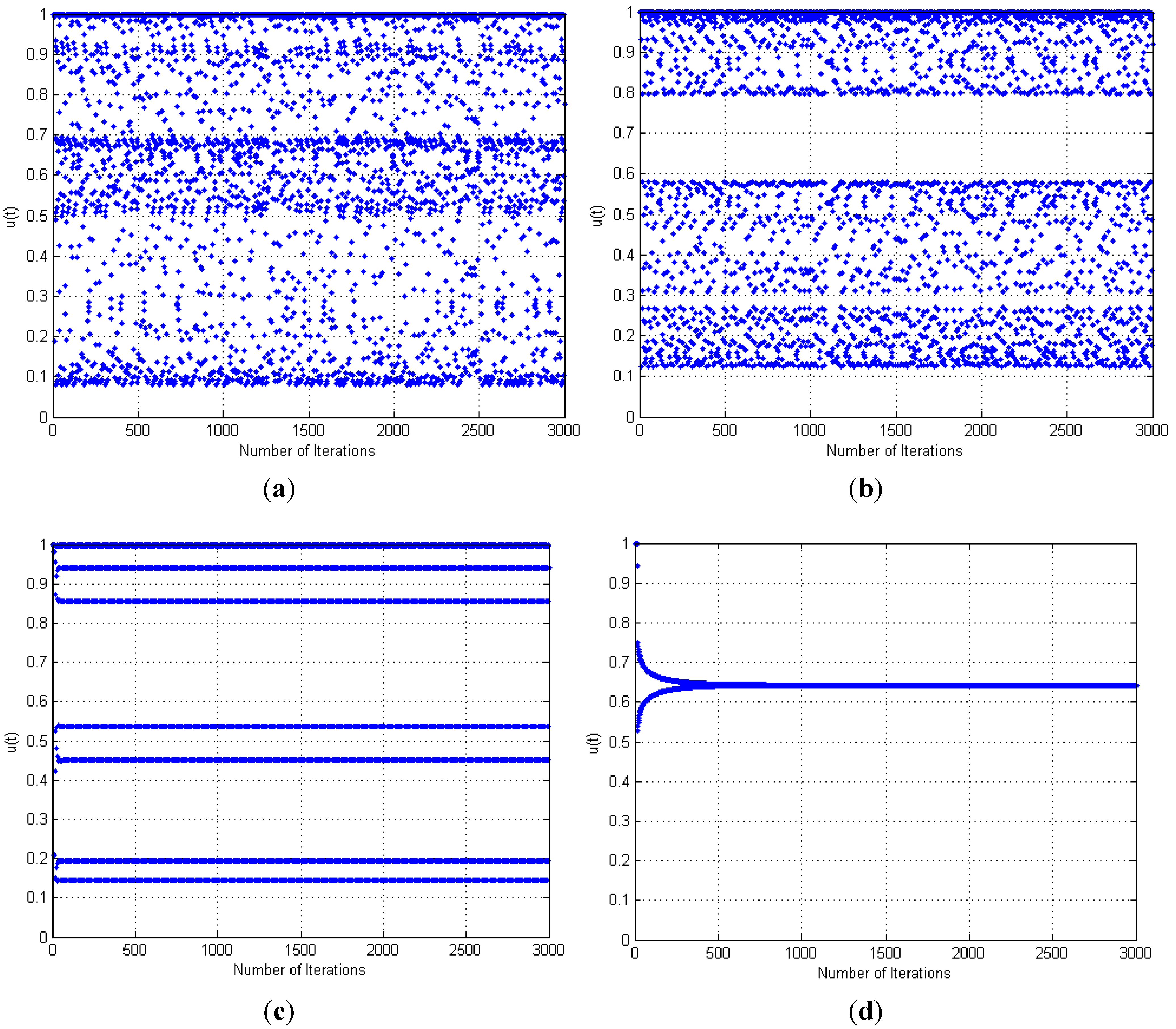
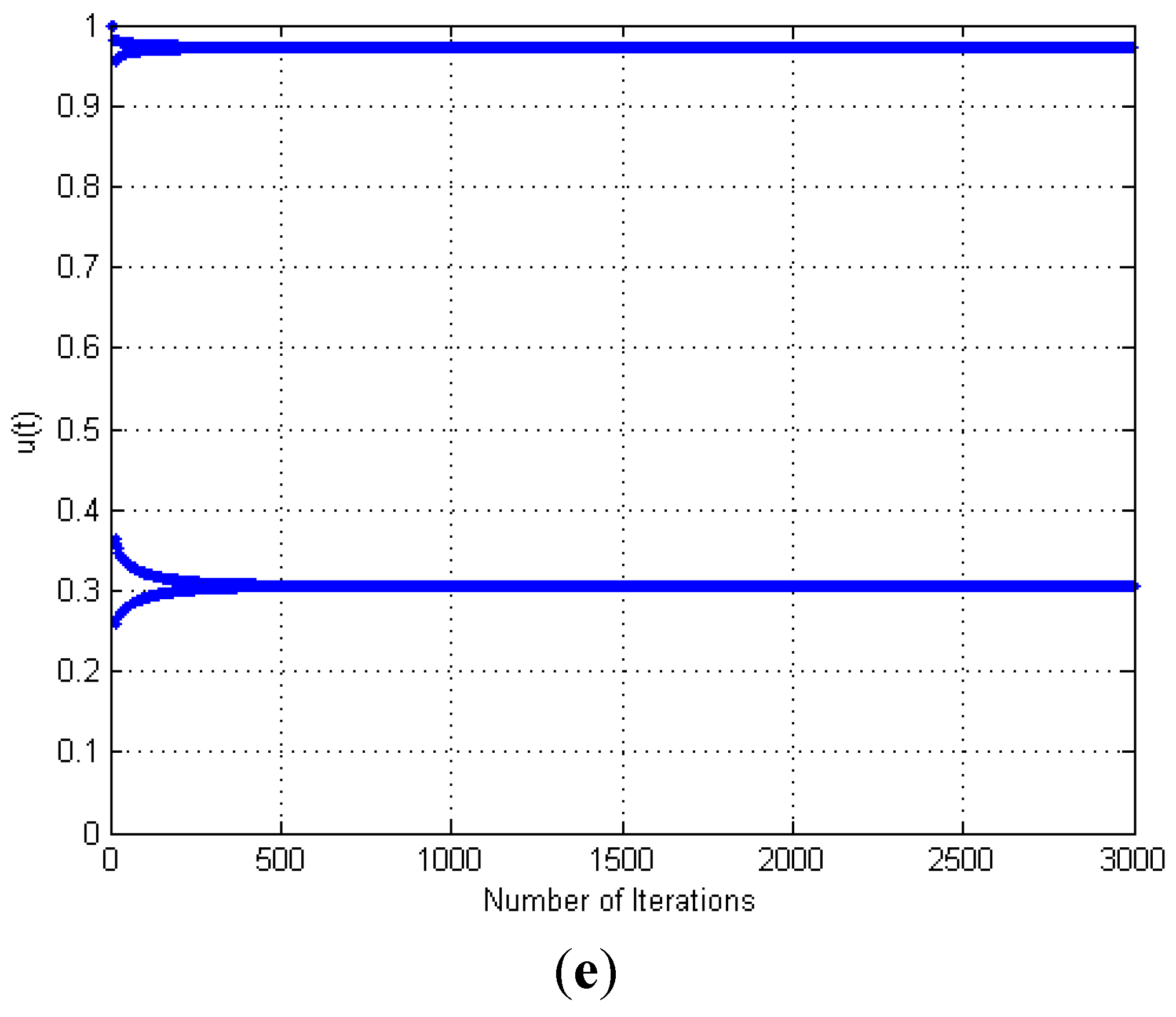
For Equations (11) and (12), output u ( t ) is expressed by a value of the self-feedback connection weight T ( t ) in the chaotic function. Figure 3 demonstrates the various bifurcation states for the weight T ( t ) during 3000 iteration. For a self-feedback connection weight in an interconnection strength T = 0.068 chaotic activity is generated, while T <0.068 the transient state u ( t ) gradually transient form chaotic state though periodic bifurcation to a steady-state. The chaotic function converges with the decrease of T ( t ) gradually. The chaotic function converges with the decrease of T ( t ) gradually. Figure 3 shows the process of u ( t ) transient state of the interconnection strength between input neurons and output neurons. Where the initial condition is as follow: ε = 0.004 , k = 0.9 , E = 0 , I 0 = 0.65 . The phenomenon indicates the chaotic behavior in a chaotic network. An annealed function is used to converge to a stable equilibrium point for a dynamic T ( t ) .
Figure 3. For various T(t) during 3000 iterations, demonstrates the various bifurcation states: (a) T(t) = 0.068; (b) T(t) = 0.061; (c) T(t) = 0.0588; (d) T(t) = 0.0499; (e) T(t) = 0.033.
Algorithms 07 00492 g003aAlgorithms 07 00492 g003b
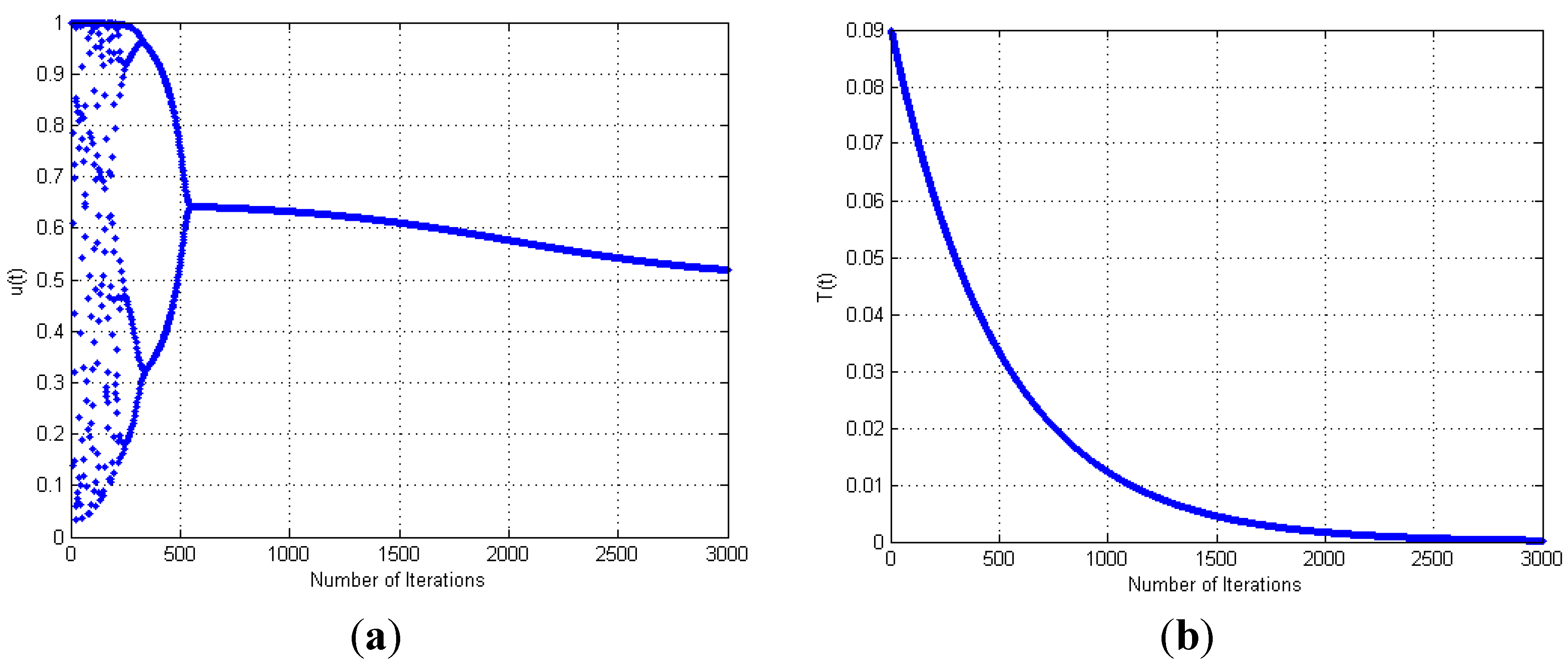
Figure 4 shows the time evolution of u ( t ) , T ( t ) . The initial condition is as follows: ε = 0.004 , k = 0.9 , E = 0 , I 0 = 0.65 , T 0 = 0.09 , y 0 = 0.5 , β = 500 , α = 0.98 [6]. Output u ( t ) can converge to a steady-state point. It shows the process of a number of iterations and bifurcation of chaotic dynamics. Exponential damping of T ( t ) is a process of simulated annealing [8]. The dynamic structure embeds into the competitive learning network in the experiment. Furthermore, the initial value of the parameters influences the dynamics process in training network. The above selected parameters were valid for all the bifurcation processes. The experiment shows the annealed chaotic mechanism can converge rapidly in the competitive network. Figure 4a demonstrates the output of a single neuron u ( t ) . Figure 4a demonstrates annealing process of damping variable.
T ( t ) = 1 b + 1 [ b + tanh ( a ) t ] T ( t - 1 )   t = 1 , 2 , 3
T = self-feedback connection weight or refractory strength ( T > 0 ) .
Figure 4. (a) Output of single neuron u ( t ) ; (b) Self-feedback connection weight T ( t ) during 3000 iteration, or the damping variable corresponding to the temperature in the annealing process. ( α = 0.98 , β = 500 , E = 0 ).
Algorithms 07 00492 g004

3. Annealed Chaotic Competitive Learning Network
The conventional competitive learning network can drop into local minima in the training network. The network embeds into an annealed chaotic mechanism and obtains an optical solution in a global scope [26]. The transient chaotic network model sensitively relies on a self-feedback connection weight. It is similar to a stochastic simulated annealing temperature and changes dynamically in the process. The annealed chaotic competitive network can jump out the local-minima and reduce the convergence time.
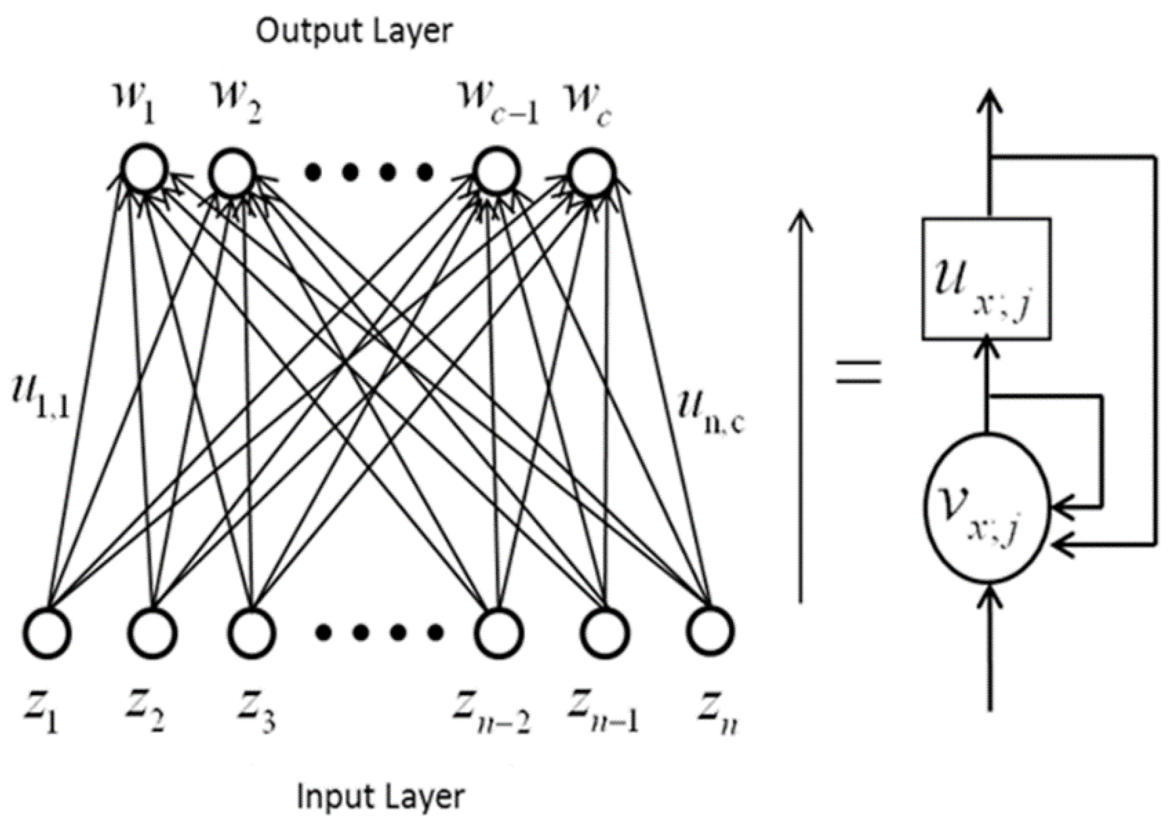
A two-layer annealed chaotic competitive learning network topology is shown in Figure 5. N neurons in the input layer are divided into c classifications in the output layer. There are c cluster-centers in the output layer. In the training process, the transient state u x ; j and the internal state v x ; j of the interconnection strength between the input layer and the output layer are tending towards stability by an annealed chaotic mechanism. The output states are updated by a gradient descending manner with a small learning-rate parameter. In the bifurcation states the parameter is used for parallel synchronous computation.
Figure 5. The annealed chaotic neural network topology.
Algorithms 07 00492 g005
The convergence process of annealed chaotic competitive neural network (ACCLN) is shown in [26]. The neuron states are changed by the function v x ; j . A simulated annealing strategy is applied for the training network by Equation (14). The network model is composed by n neurons in the input layer, c neurons in the output layer and n × c interconnection strengths. The model is shown as follows:
E = 1 2 x = 1 n j = 1 c u x ; j | z x w j | 2
u x ; j ( t ) = 1 1 + e v x ; j ( t ) / ε
v x ; j ( t + 1 ) = k v x ; j ( t ) + E T ( t ) ( u x ; j ( t ) I 0 )
w j = η ( z x w j ) u x ; j
T ( t ) = 1 β + 1 [ β + t a n h ( α ) t ] T ( t 1 )
w j ( t + 1 ) = w j ( t ) + w j ( t )
Where E is energy function of the n input neuron nodes and c output nodes. u x ; j and v x ; j are the transient state and internal state of interconnection strength, respectively. The transient state and internal state are training by a self-feedback manner.

4. The Application of the ACCLN to Power Cable Fault

4.1. The Experimental Platform

Block diagram of the data acquisition system is shown in Figure 6. The system is based on the PCI-6221 data acquisition card to complete the data acquisition. Cable fault data is acquired by a signal conditioning circuit, then, the data converts into a digital signal by the acquisition card. Furthermore, the data is processed by computer, or sent to the data to monitoring room and realized by remote monitoring and control.
Figure 6. The experimental platform.
Algorithms 07 00492 g006
Table 1 shows 54 data, which contains training samples and test samples. There are two kinds of cable faults types and a normal condition, interphase short circuit, three phase short circuit, and normal condition, respectively. In this paper, those data are applied to test the IPSO-SVM method and the ACCLN method. The steps of IPSO-SVM method are introduced, the training results and test results are shown as follows:
Table 1. Cable fault sample data.
Fault typesTraining samplesTest samplesTotal sample number
interphase short circuit9716
three phase short circuit8513
normal condition151025
Total322254

4.2. Performance of the IPSO-SVM Algorithm

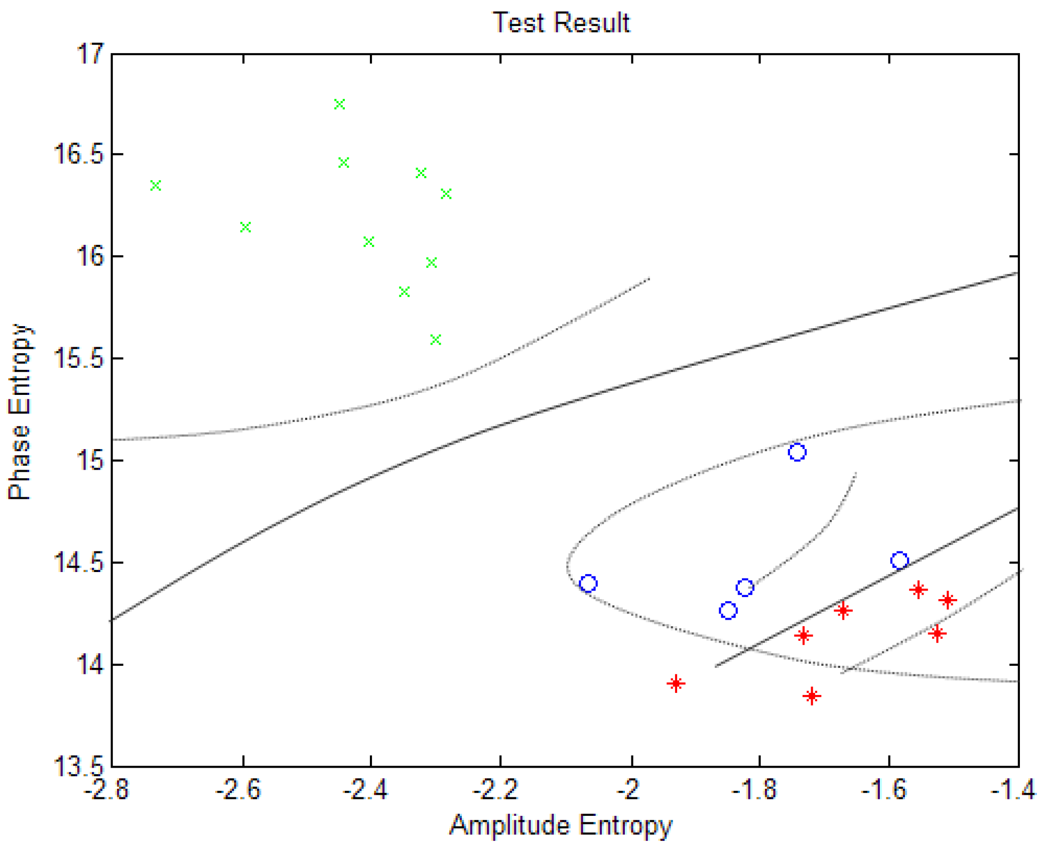
In order to test performance of the IPSO-SVM algorithm, Figure 7 shows the training result of IPSO-SVM method. Figure 8 shows the test result of IPSO-SVM method.
Figure 7 shows the training result the by IPSO-SVM method via 32 training data in Table 1. Figure 8 shows the test result the by IPSO-SVM method via 22 test data in Table 1. The cable fault features have different degrees of difference. However, it is not easy to distinguish the similar cable fault. So the ACCLN method is proposed to solve the problem.
Figure 7. The training results of improved Particle Swarm Optimization-Support Vector machine (IPSO-SVM) method.
Algorithms 07 00492 g007
Figure 8. The test results of IPSO-SVM method.
Algorithms 07 00492 g008

4.3. Power Cable Fault is Processed by the ACCLN Method

In this section we apply the ACCLN method to deal with power cable fault types. The data in [16] is used to recognize the power cable fault types. There are three kinds of fault types in [16], interphase short circuit, three phase short circuit, and normal condition, respectively. A total of 54 sample data are used in the experiment. The ACCLN consists of a neuron array 54 × 1 in the input layer and three neuron nodes in the output layer. The transient state u x ; j and the internal state v x ; j are 54 × 3 array. Each testing point of phase entropy and amplitude entropy are composed of an input vector, and normalized in the input layer. The phase entropy and amplitude entropy are normalized as follow. For example, for each phase entropy and amplitude entropy, the normalized value is shown as Equations (20) and (21):
p n o r m ; i = ( p i p min ) / ( p max p min )
a n o r m ; i = ( a i a min ) / ( a max a min )
and an input vector z i is shown:
z i = [ p n o r m ; i     a n o r m ; i ]
Where p i indicates the i-th phase entropy, p min and p max is the minima and maxima of the 54 phase values, respectively. p n o r m ; i is the i-th normalized phase value. The process of normalizing amplitude entropy is the same as phase entropy. z i is the i-th input vector, composing the normalized phase value p n o r m ; i and the normalized amplitude value a n o r m ; i .
The flow chart of ACCLN algorithm is shown in Figure 9. The step of ACCLN algorithm for power cable fault classification is shown as follow:
Step 1: Preprocess the input phase entropy and amplitude entropy for each test point using Equations (20–22).
Step 2: Set the cluster-center w j (j=1,2,3...) randomly for interphase short circuit, three phase short circuit, and normal condition.
Step 3: Initialize self-feedback connection T ( 0 ) , internal states and transient state for all interconnection strengths.
Step 4: Calculate the energy function (14).
Step 5: Update internal states and transient state for all interconnection strengths using Equations (15) and (16).
Step 6: Update the cluster-centers by a small learning-rate parameter using Equations (17) and (19).
Step 7: Decrease the self-feedback connection weight T ( t ) using Equation (18).
Step 8: If the network does not converge then goes to Step 4; otherwise stop.
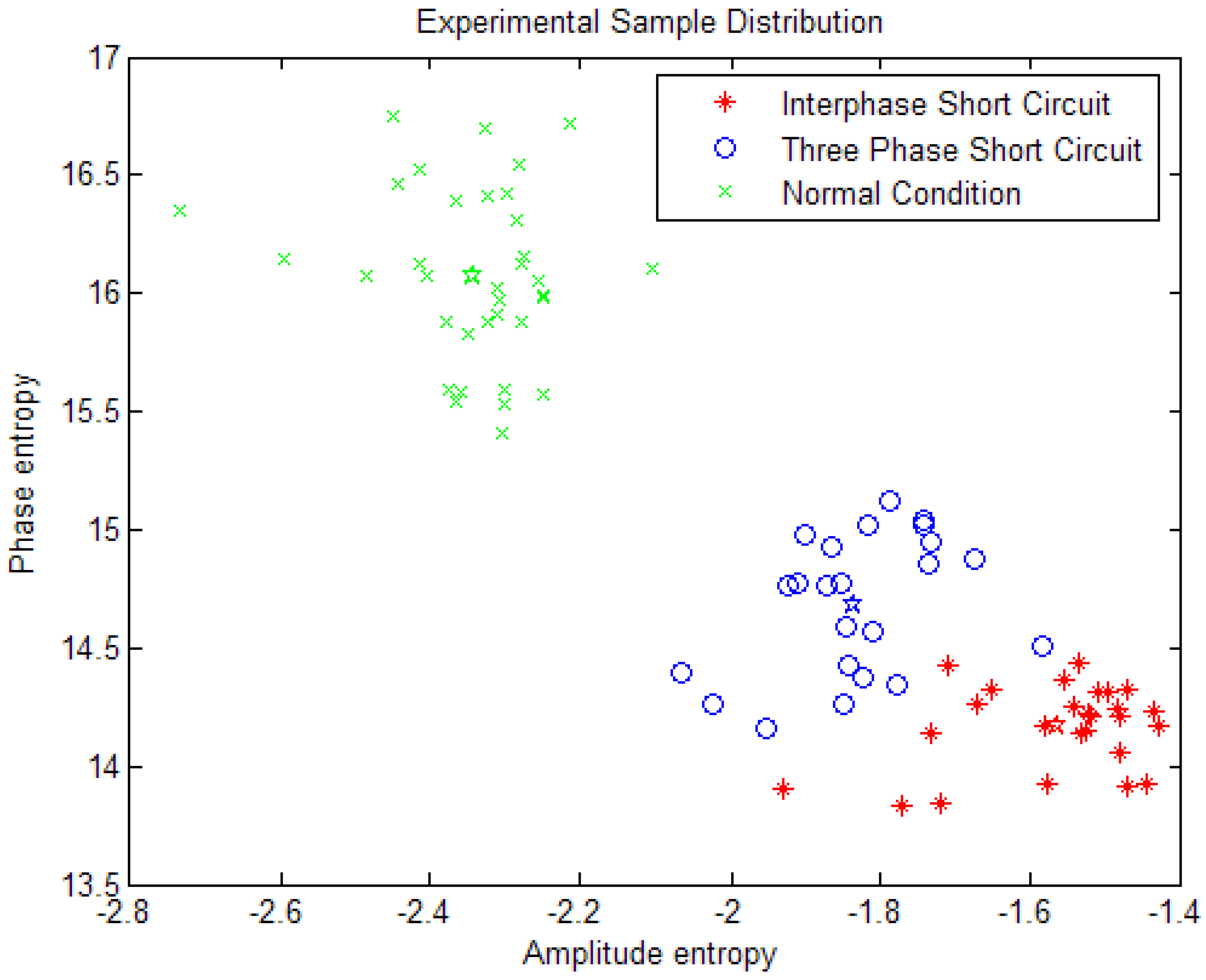
Figure 10 shows the experimental sample data distribution. There are 6 category data, interphase short circuit of training data and test data, three phase short circuit of training data and test data, normal condition of training data and test data, respectively. The recognition accuracy was 87.0% with the SVM method and 90.7% with the IPSO-SVM method in [16].
Figure 9. Flow chart of annealed chaotic competitive neural network (ACCLN).
Algorithms 07 00492 g009
Figure 10. Experimental sample data distribution. X axis indicates amplitude entropy; Y axis indicates phase entropy.
Algorithms 07 00492 g010
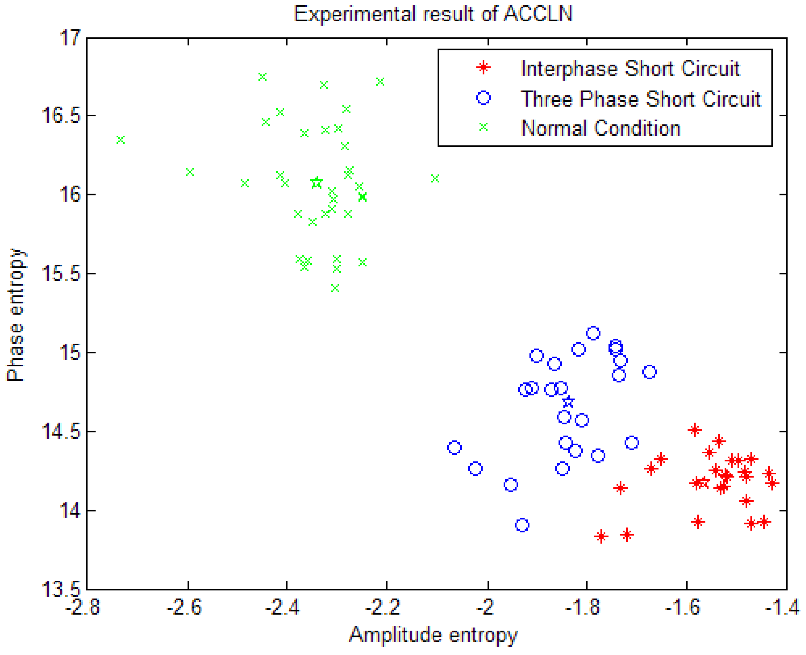
Figure 11 shows the experimental result of ACCLN. There are 54 sample data. Those samples are divided into three classifications. The green “ Algorithms 07 00492 i001” indicates normal condition of power cable, 25 samples. The blue “ Algorithms 07 00492 i002” indicates the power cable of three-phase short circuit, 13 samples. The red “ Algorithms 07 00492 i003” indicates the power cable of interphase short fault, 16 samples. The different colors “☆” corresponds to each cluster-center.
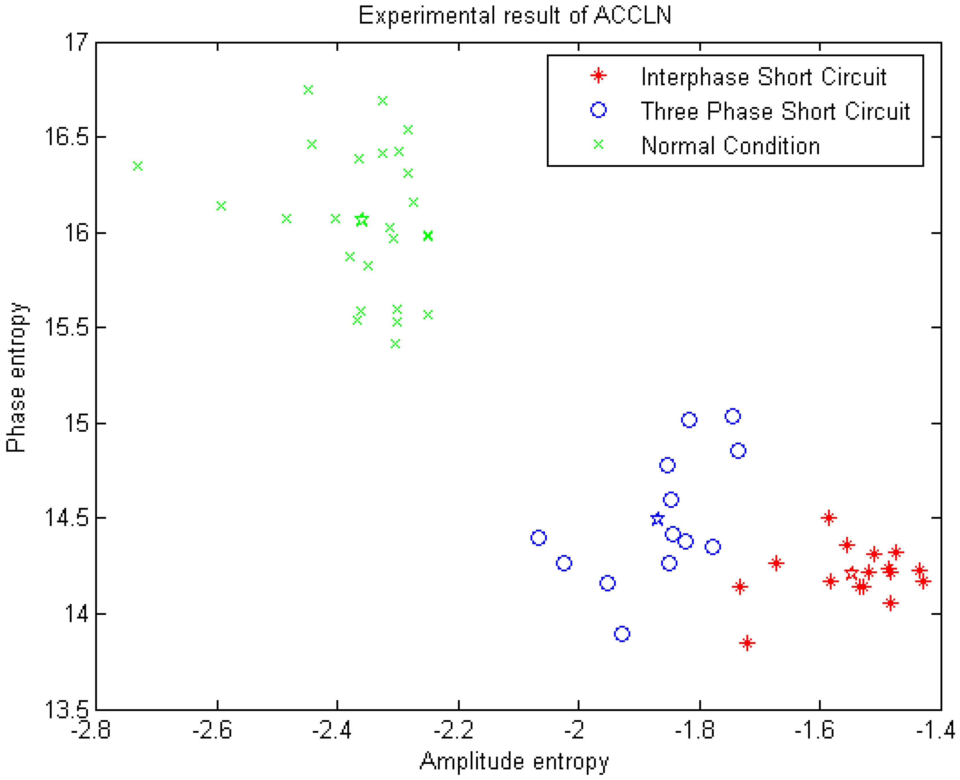
Figure 11. Experimental result of ACCLN. X axis indicates amplitude entropy; Y axis indicates phase entropy.
Algorithms 07 00492 g011
Table 2 shows the recognition accuracy of SVM, IPSO-SVM, and ACCLN methods. The recognition accuracy of ACCLN, IPSO-SVM and SVM is 96.2%, 90.7%, 87.0%, respectively. The training times are 0.032, 0.0523, 0.0575, respectively. The performance of the power cable fault recognition of ACCLN method is better than SVM and the IPSO-SVM method.
Table 2. Recognition accuracy of SVM, IPSO-SVM and ACCLN.
AlgorithmRecognition AccuracyTraining Time
ACCLN96.2%0.032
IPSO-SVM90.7%0.0523
SVM87.0%0.0575
In order to test the effectiveness of the proposed method, each group of dataset add 10 test samples, 30 test samples are added on the basis of original samples. So there are 84 test samples in experiment. Figure 12 shows 84 sample distributions. Figure 13 shows the result of ACCLN method. The recognition accuracy of ACCLN is 96.4%.
Figure 12. Experimental sample data distribution (84 samples); X axis indicates amplitude entropy; Y axis indicates phase entropy.
Algorithms 07 00492 g012
Figure 13. Experimental result of ACCLN (84 samples). X axis indicates amplitude entropy; Y axis indicates phase entropy.
Algorithms 07 00492 g013

5. Conclusions

In this paper, we apply the ACCLN algorithm to recognize power cable fault types. A simulated annealing strategy and chaotic mechanism are used for clustering analysis. The proposed approach possesses the merits of obtaining global optimal solution and high accuracy. The annealing process in the ACCLN algorithm is associated with the series of the bifurcation. In the classification of power cable faults, the results show a better performance than with the SVM and IPSO-SVM methods.
It is difficult to select suitable parameters to obtain the global optimal solution with the ACCLN method. In order to demonstrate the effectiveness of selecting parameters, different bifurcation states are displayed in the experiment. A set of valid parameters is fixed to produce a near global optimal solution. Therefore, how to select suitable parameters automatically, and improve the accuracy of the ACCLN method, is our future work.

Acknowledgments

This paper is supported by Scientific Research Foundation for Returned Scholars, Ministry of Education of China ([2011]508) and Natural Science Foundation of Shaanxi Province (2011JM8005), sponsored by the National Science Council of Taiwan under the Grant NSC101-2221-E-167-040.

Author Contributions

Xuebin Qin and Jzau-Sheng Lin conceived and designed the experiments; Mei Wang and Xiaowei Li performed the experiments; Xuebin Qin and Mei Wang analyzed the data; Xiaowei Li contributed data of power cable fault; Xuebin Qin wrote the paper.

Conflicts of Interest

The authors declare that there is no conflict of interest regarding the publication of this paper.

References

  1. Wang, M.; Stathaki, T. Online fault recognition of electric power cable in coal mine based on the minimum risk neural network. J. Coal Sci. Eng. 2008, 14, 492–496. [Google Scholar] [CrossRef]
  2. Ratnaweera, A.; Halgamuge, S. Self-Organizing Hierarchical Particle Swarm Optimizer with Time-Varying Acceleration Coefficients. IEEE Trans. Evol. Comput. 2004, 8, 240–255. [Google Scholar] [CrossRef]
  3. Chen, P.; Zhao, C.H.; Li, J.; Liu, Z.M. Solving the Economic Dispatch in Power System via a Modified Genetic Particle Swarm Optimization. In Proceedings of the 2009 International Joint Conference on Computational Sciences and optimization, Sanya, Hainan, China, 24–26 April 2009; pp. 201–204.
  4. Gao, S.; Zhang, Z.Y.; Cao, C.G. Particle Swarm Optimization Algorithm for the Shortest Confidence Interval Problem. J. Computer. 2012, 7, 1809–1816. [Google Scholar] [CrossRef]
  5. Fronza, L.; Sillitti, A.; Succi, G. Failure prediction based on log files using Random Indexing an Support Vector Machines. J. Syst. Softw. 2013, 86, 2–11. [Google Scholar] [CrossRef]
  6. Liu, H.; Li, S. Decision fusion of sparse representation and support vector machine for SAR image target recognition. Neurocomputing 2013, 113, 97–104. [Google Scholar] [CrossRef]
  7. Yang, X.; Yu, Q.; He, L.; Guo, T. The one-against-all partition based binary tree support vector machine algorithms for multi-class classification. Neurocomputing 2013, 113, 1–7. [Google Scholar] [CrossRef]
  8. Zhang, J.-M.; Liang, S. Research on Fault Location of Power Cable with Wavelet Analysis. In Proceedings of the IEEE Digital Manufacturing and Automation, Zhangjiajie, Hunan, China, 5–7 August 2011; pp. 956–959.
  9. Jiang, J.A.; Chen, C.-S.; Liu, C.-W. A new protection scheme for fault detection, direction discrimination, classification, and location in transmission lines. IEEE Trans. Power Deliv. 2003, 18, 34–42. [Google Scholar] [CrossRef]
  10. Gnatenko, M.A.; Shupletsov, A.V.; Zinoviev, G.S.; Weiss, H. Measurement system for quality factors and quantities of electric energy with possible wavelet technique utilization. In Proceedings of the 8th Russian-Korean International Symposium on Science and Technology, Tomsk Polytechnic University, Tomsk, Russia, 26 June–3 July 2004; pp. 325–328.
  11. Li, B.; Shen, Y. Electric Heating Cable Fault Locating System Based on Neural Network. In Proceedings of the IEEE International Conference on Natural Computation, Tianjin, China, 14–16 August 2009; pp. 43–47.
  12. Wang, M.; Li, X. Power Cable Fault Recognition Using the Improved PSO-SVM Algorithm. Appl. Mech. Mater. 2013, 427–429, 830–833. [Google Scholar] [CrossRef]
  13. Cai, G.-L.; Shao, H.-J. Synchronization-based approach for parameter identification in delayed chaotic network. Chin. Phys. B 2010, 19, 1056–1074. [Google Scholar]
  14. Uchiyama, T.; Arbib, M.A. Color Image Segmentation using competitive learning. IEEE Trans. Pattern Anal. Mach. Intell. 1994, 16, 1197–1206. [Google Scholar] [CrossRef]
  15. Lin, J.; Tsai, C. An Annealed Chaotic Competitive Learning Network with Nonlinear Self-feedback and Its Application in Edge Detection. Neural Process. Lett. 2001, 13, 55–69. [Google Scholar] [CrossRef]
  16. Lu, S.W.; Shen, J. Artificial neural networks for boundary extraction. In Proceedings of the IEEE International Conference on SMC, Beijing, China, 14–17 October 1996; pp. 2270–2275.
  17. Xiang, W.; Zhou, Z. Camera Calibration by Hybrid Hopfiled Network and self-Adaptive Genetic Algorithm. Meas. Sci. 2012, 12, 302–308. [Google Scholar]
  18. Wright, A.H. Genetic Algorithms for Real Parameter Optimization. In Foundations of Genetic Algorithms; Rawlins, G.J.E., Ed.; Morgan Kaufmann: Missoula, Montana, 1991; pp. 205–218. [Google Scholar]
  19. Lin, J.-S.; Liu, S. Classification of Multispectral Images Based on a Fuzzy-Possibilistic Neural Network. IEEE Trans. Syst. Man Cybern. Part C Appl. Rev. 2002, 32, 499–506. [Google Scholar]
  20. Zhang, C.; Liu, Y.; Zhang, H.; Huang, H. Research on the Daily Gas Load Forecasting Method Based on Support Vector Mechine. J. Comput. 2011, 6, 2662–2667. [Google Scholar] [CrossRef]
  21. Al-Geelani, N.A.; Piah, M.A.M.; Adzis, Z.; Algeelani, M.A. Hybrid regrouping PSO based wavelet neural networks for characterization of acoustic signals due to surface discharges on H.V. insulators. Appl. Soft Comput. J. 2013, 13, 78–87. [Google Scholar] [CrossRef]
  22. Maldonado, Y.; Castillo, O.; Melin, P. Particle swarm optimization of interval type-2 fuzzy systems for FPGA applications. Appl. Soft Comput. J. 2013, 13, 456–465. [Google Scholar] [CrossRef]
  23. Hamta, N.; Fatemi Ghomi, S.M.T.; Jolai, F.; Akbarpour Shirazi, M. A hybrid PSO algorithm for a multi-objective assembly line balancing problem with flexible operation times, sequence-dependent setup times and learning effect. Int. J. Prod. Econ. 2013, 141, 357–365. [Google Scholar] [CrossRef]
  24. Qi, F.; Xie, X.; Jing, F. Application of improved PSO-LSSVM on network threat detection. Wuhan Univ. J. Nat. Sci. 2013, 18, 418–426. [Google Scholar] [CrossRef]
  25. Tavakkoli-Moghaddam, R.; Azarkish, M.; Sadeghnejad-Barkousaraie, A. Solving a multi-objective job shop scheduling problem with sequence-dependent setup times by a Pareto archive PSO combined with genetic operators and VNS. Int. J. Adv. Manuf. Technol. 2011, 53, 733–750. [Google Scholar] [CrossRef]
  26. Lin, J.-S. Annealed chaotic neural network with nonlinear self-feedback and its application to clustering problem. Patten Recognit. 2001, 34, 1093–1104. [Google Scholar] [CrossRef]
  27. Tsai, C.; Liaw, C. Polygonal approximation using an annealed chaotic Hopfield network. In Proceedings of the IEEE International Workshop on Cellular Neural Networks and Their Application, Hsinchu, Taiwan, 28–30 May 2005; pp. 122–125.
  28. Chen, L.; Kazuyaki, A. Chaotic Simulated Annealing by a Neural Network Model with Transient Chaos. Neural Netw. 1995, 8, 915–930. [Google Scholar] [CrossRef]
  29. George, A.; Katerina, T. Simulating annealing and neural networks for chaotic time series forecasting. Chaotic Model. Simul. 2012, 1, 81–90. [Google Scholar]
  30. Atsalakis, G.; Skiadas, C. Forecasting Chaotic time series by a Neural Network. In Proceedings of the 8th International Conference on Applied Stochastic Models and Data Analysis, Vilnius, Lithuania, 30 June–3 July 2008; pp. 77–82.