Efficient in silico Chromosomal Representation of Populations via Indexing Ancestral Genomes

Abstract

One of the major challenges in handling realistic forward simulations for plant and animal breeding is the sheer number of markers. Due to advancing technologies, the requirement has quickly grown from hundreds of markers to millions. Most simulators are lagging behind in handling these sizes, since they do not scale well. We present a scheme for representing and manipulating such realistic size genomes, without any loss of information. Usually, the simulation is forward and over tens to hundreds of generations with hundreds of thousands of individuals at each generation. We demonstrate through simulations that our representation can be two orders of magnitude faster and handle at least two orders of magnitude more markers than existing software on realistic breeding scenarios.

1. Introduction

Study of populations via simulations is an important problem, with applications ranging from tracking population history to modeling heritable diseases. Numerous population simulation methods exist in the literature that are geared towards handling human data [1,2,3]. In comparison, only a small number of systems cater to plant and animal breeding populations [4,5]. The former is dominated by the backward simulation approaches, but the latter usually uses forward simulations. Although the backward simulation is a mathematically clever scheme of avoiding redundant computations, as well as redundant ancestors in the simulation, the approach is cumbersome when the requirement is to track multiple segments (chromosomes) for breeding simulations. The whole genome, spread across multiple chromosomes, is required to obtain a realistic genetic or breeding value. Thus, a time and space efficient representation and computation is necessary for realistic simulations. This also enables comparative simulations where thousands of simulations can be carried out based on varying breeding processes to detect the few favorable ones that can be implemented in practice.

Classical plant breeding is performed by crossing closely or distantly related individuals to produce new crop varieties with desirable properties. Breeding aims to generate individuals with new and enhanced genetic material by combining genes encoding favorable traits (e.g., disease resistance, drought tolerance, high yield). The quality of the new genetic material is often measured by a phenotype value computed via some mathematical model based on quantitative genetics theory [6,7]. The general problem setting of crossing genetic material and computing phenotype values of the progeny is illustrated in Figure 1. The interested reader is referred to [8] for more details capturing the meiotic crossovers.

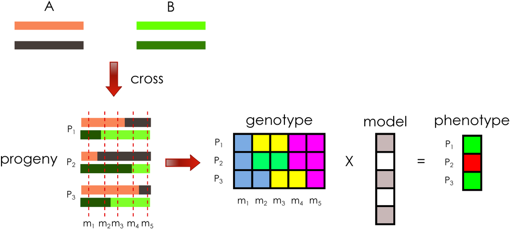
Figure 1. Illustration of the general problem setting. Crossing the diploid founder genomes, A and B, produces three progeny, $P_1,P_2,P_3$, and each progeny haploid has a single crossover introduced in the meiosis, illustrated by the two different colors per haploid. The genotype matrix for five markers, $m_1,\dots ,m_5$, represents the aggregate of haploid information per progeny, at specific genomic locations. Each progeny is assigned a phenotype value based on their genotype and a phenotype model.

Figure 1. Illustration of the general problem setting. Crossing the diploid founder genomes, A and B, produces three progeny, $P_1,P_2,P_3$, and each progeny haploid has a single crossover introduced in the meiosis, illustrated by the two different colors per haploid. The genotype matrix for five markers, $m_1,\dots ,m_5$, represents the aggregate of haploid information per progeny, at specific genomic locations. Each progeny is assigned a phenotype value based on their genotype and a phenotype model.

Ideally, one would be able to predict, via inexpensive and fast computer simulations, the actual phenotypes of progeny resulting from crosses between existing genotyped individuals. This could potentially yield great improvement in time and cost required for developing new and successful varieties. Due to the advent of high-throughput genomic measurement technologies, there is a continuing substantial increase in the amount of genotype data that the simulation process should be able to utilize. The interested reader is referred to [9] for the relevance of data representation in bioinformatics in general. In order to address the important issue of genotype data representation, in this paper, we propose an efficient data structure that is especially designed for plant population simulations, while also applicable for animal breeding or other related applications.

We describe a time- and space-efficient (i) genome representation as segments from founder genomes and (ii) computation of phenotype values (when the underlying phenotype model is additive). Our segment-based representation takes less time and space than a traditional representation of individuals as vectors of genotype values at specific markers. The segment approach is also more general, since it may be used with any selection of markers along the genome. Furthermore, the segment representation allows precise tracking of the parental origin of each location in the genome. This will make any task related to breeding simulations more efficient, including simulating a particular breeding process and optimizing the choice of breeding processes. Applications of breeding simulations, where efficiency is paramount, include obtaining statistics on outcomes of breeding processes. Examples include statistics on the number of instances, where a specific genotype or increase in average population value for a trait of interest (such as yield or disease resistance) is observed, optimizing the choice of founding parents from a germplasm collection and optimizing the choice of breeding processes. Efficient genome simulations also allow validating the robustness of given breeding processes, by obtaining statistics on the outcomes of several instances of the same process. Additionally, the segment representation could be used to efficiently store individual haplotype values for phased populations, such as $F_1$ populations, resulting from a cross between two founders.

In the experimental analysis, we evaluate the performance of existing population simulation methods and our segment representation, also contrasting it with a basic vector representation. The results show that the existing methods and the vector representation do not scale for large number of markers and progeny. Our experimental results demonstrate that the segment representation is at least an order of magnitude faster and able to handle at least two orders of magnitude more markers than existing software on realistic breeding scenarios. In this paper, we illustrate the approach with a genome consisting of one diploid chromosome; the ideas are easily extendable to genomes with several chromosomes.

This paper is organized as follows. Section 2 provides the main idea of the genome representation via segments, while Section 3 describes how to use it for efficient phenotype computation. Section 4 details the experimental validation, and Section 5 provides the conclusions.

2. Genome Representation

In this section, we present the main idea of using segments to represent a genome and contrast the efficiency of this approach with a traditional representation as vectors of genomic marker values. One of the most common biological distance measures is the Morgan: one Morgan is the genomic distance over which, on average, one crossover occurs per meiosis [10]. Let L be the length of the chromosome, in Morgans; the expected number of crossovers per meiosis is L. Let S denote the total number of segments per individual and $S(·)$, the number of segments per haploid. Founder A haploids, $A_1$ and $A_2$, consist of $S=S\left(A_1\right)+S\left(A_2\right)$ segments. Initially, each haploid consists of one segment, $S\left(A_1\right)=S\left(A_2\right)=1$. Each crossover introduces one additional segment per haploid; thus, the progeny of $A\times A$ (A crossed, e.g., pollinated, with A) consists of, on average, $S+2L$ segments. In addition to the segment boundaries, the parental origin (in this case, label $A_1$ or $A_2$) is known for each segment in the simulation context. Using the segment boundary and label data, we are able to perfectly reconstruct each progeny from the known genomes of the parents. Thus, the segment starts, and labels define a necessary and sufficient representation of the progeny genomes.

Each progeny can be represented with a dynamic data structure that allows efficiently iterating over the existing segments and adding new segments. An example of such a data structure is a balanced search tree, where the key of each node represents the location where the corresponding segment begins. The advantages of a balanced tree include logarithmic time search for the segment overlapping a given genome position. An alternative representation is a linked list, with the caveat that searching for the segment overlapping a given position takes linear time. However, since a common application of segment representation is to compute the phenotype using all segments and markers, in increasing order of genome location, a linked list may be a sufficient representation. In our experiments, we used a balanced search tree (C++ standard container map) to demonstrate that even this more complex data structure with some overhead has negligible time and space requirements compared with the vector representation. Additional data for each segment (node) will include the label of its parental origin.

The key ideas of the genome representation are illustrated with the examples in Figure 2. Figure 2(a) shows the representation of a haploid obtained after the meiosis between two founder haploids. Figure 2(b) shows the haploid representation when the meiosis operation is performed on the haploid obtained in Figure 2(a) and the haploid of another founder.

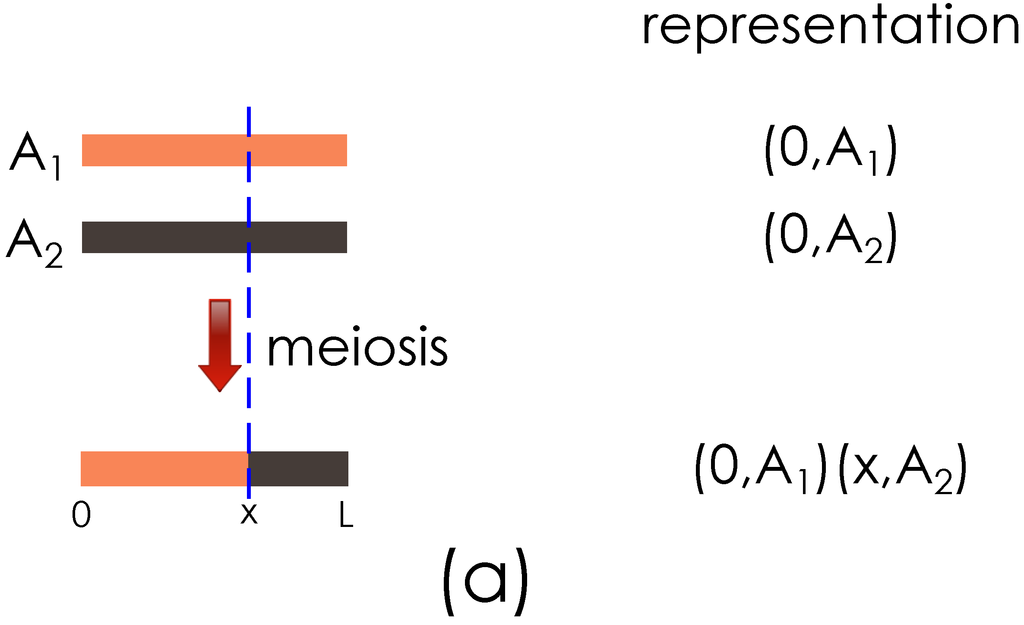
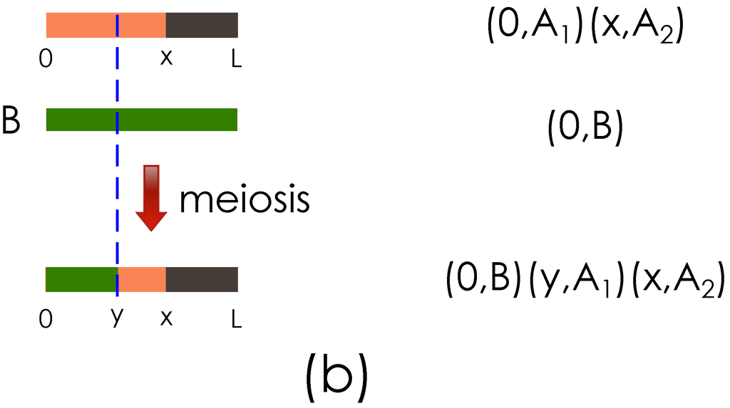
Figure 2. Illustration of the genome segment representation. (a) Representation of founder genome A haploids, $A_1$, $A_2$, and the result of meiosis with a crossover at x are shown; (b) Output from (a) and founder haploid B are shown going through meiosis, with a new crossover introduced at y.

Figure 2. Illustration of the genome segment representation. (a) Representation of founder genome A haploids, $A_1$, $A_2$, and the result of meiosis with a crossover at x are shown; (b) Output from (a) and founder haploid B are shown going through meiosis, with a new crossover introduced at y.

2.1. Computational Complexity

Assume L crossovers are introduced, while the parents have in total S segments and M markers. The time complexity of segment representation meiosis is $O(S+L\text{log}L)$. This can be achieved by scanning the parents’ segment data structures, while updating and switching the haplotype pointers as necessary. The vector representation meiosis takes time $O(M+L\text{log}L)$. The time, $L\text{log}L$, reflects generating and ordering L random crossover locations.

In addition to the L introduced segment boundaries, the S segment boundaries from the parents need to be stored, as they are part of the representation of the progeny. Thus, each progeny in the segment representation requires storage of $O(S+L)$ entities. In contrast, storing the marker values for each progeny requires storing $O\left(M\right)$ entities in the vector representation.

Since, in general, $S\ll M$, the segment representation can be several orders of magnitude faster, as demonstrated in Section 4, as well as requiring several orders of magnitude less space.

The total number of segments grows somewhat slower than the average L per generation, because neighboring segments originating from the same parental haplotype are combined during the meiosis operation. Relating to forward simulations of hundreds of generations, such as for evolutionary studies, expected limits for the number of founder segments in isolated random mating populations are presented in [11,12]. We illustrate the expected number of segments with simulation results in Figure 3 (they are in agreement with Figure 2.1 in [12]). Additionally, we show that populations with only two founders have fewer segments (agreeing with Equation (5) in [11]). Since breeding schemes operate on relatively short time scales (e.g., tens of generations), over-fragmentation is not an issue with this representation in practice, as also demonstrated in Figure 4.

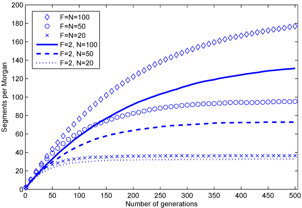
Figure 3. Average number of segments per one Morgan in a haploid during 500 generations in simulations of random mating populations. F is the number of individuals in the founder population, and N is the number of individuals in every subsequent population. The parents of each progeny are chosen at random (with replacement) from the previous generation.

Figure 3. Average number of segments per one Morgan in a haploid during 500 generations in simulations of random mating populations. F is the number of individuals in the founder population, and N is the number of individuals in every subsequent population. The parents of each progeny are chosen at random (with replacement) from the previous generation.

Figure 4. Time requirements of selfing the result of a cross for 10 generations, while at each generation, applying selection after computing the phenotype values. Cumulative time taken for progeny generation and phenotype computation after each generation is shown.

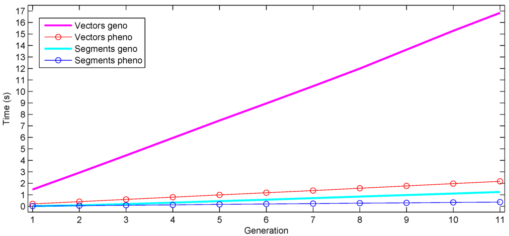
Figure 4. Time requirements of selfing the result of a cross for 10 generations, while at each generation, applying selection after computing the phenotype values. Cumulative time taken for progeny generation and phenotype computation after each generation is shown.

3. Phenotype Computation

The main ideas behind efficient phenotype computation are (i) storing the progeny as genome segments and (ii) pre-computing the founder phenotype values for all possible segments, by adding up the contributions of each genotype marker within a segment. This is applicable when the phenotype is additive (or multiplicative), which is one of the fundamental and widely used models underlying phenotype computations [6]. Furthermore, popular whole genome prediction models, such as rrBLUP [13,14], Bayes A [14], Bayes B [14], Bayes Cpi [15] and Lasso [16], utilize an additive phenotype model. The phenotype computation is specific to a given marker model, and the pre-computed values apply only for the model for which they were computed. The phenotype contribution of each possible genome segment can be evaluated using the pre-computed cumulative sum (or product) of phenotype contributions, as explained below.

An additive phenotype value for individual i, ${\mathcal{P}}_i={\sum }_j^M{g}_{i,j}{\beta }_j+\alpha$, can be efficiently computed by adding up the independent pre-computed values for each segment in i. Here, ${\beta }_j$ and α are given parameters of the phenotype model, and $g_{i,j}$ is the genotype at marker j in individual i. The additive nature of the phenotype, $\mathcal{P}$, allows the phenotype computation to be defined as a sum over subsets of markers. In order to utilize this subdivision, one can pre-compute a table, V, containing the phenotype value of each possible segment of the genome. In practice, the values can be stored as a cumulative sum from the first genotype marker to the last. For simplicity, assume here we have just two founder haploids, A and B, for example, in the case where the founders fully homozygous, as is often encountered in plant breeding. The discussion below applies to any number of founders; only the dimensionality of the pre-computed tables may change. In the two-founder case, there are three possible founder combinations for each diploid segment: $AA$, $AB$, $BB$. Therefore three pre-computed tables are needed: $V_{AA}$, $V_{AB}$ and $V_{BB}$.

Since, in the segment representation, we are dealing with genome segments instead of individual markers, we need to map the genome segment boundaries to the genotype markers, in order to efficiently index the pre-computed tables, V. Let φ be a function that maps a genomic location, x, onto the nearest genotype marker, s, whose location is larger than x. Given x and y, $x<y$, as two genetic positions in the haploid, we have $s=\phi \left(x\right)$ and $t=\phi \left(y\right)$. For example, the phenotype contribution, $\mathcal{P}(s,t-1)$, for markers $0<s<t$, corresponding to the genome segment from x to y, where both haploids originate from founder A, can be quickly computed as $\mathcal{P}(s,t)=V_{AA}[t-1]-V_{AA}[s-1]$.

The markers’ genome locations can be represented as a sorted list of positions in a searchable data structure, enabling logarithmic time search for the marker closest to a given segment boundary. When computing the phenotype value of a genome from the segment representation, the indices of the first and last markers in each segment need to be determined, as well as the parental origins of the segment, in order to correctly index the pre-computed phenotype contribution tables, V.

Here, we provide a small example of additive phenotype computation using the segment representation. Let us consider an individual with the following segment representation for the two haploids, with $x<y$:

$$(0,A)(x,B)$$

$$(0,B)(y,A)$$

then, its phenotype can be obtained as $\mathcal{P}=\mathcal{P}(1,s-1)+\mathcal{P}(s,t-1)+\mathcal{P}(t,M)=V_{AB}[s-1]+V_{BB}[t-1]-V_{BB}[s-1]+V_{AB}\left[M\right]-V_{AB}[t-1]$, where $s=\phi \left(x\right)$ and $t=\phi \left(y\right)$ are the mapping of genomic locations x and y to genotype markers and M is the number of markers.

In addition to the additive phenotype model, interactions between some markers could also be included in the phenotype calculation. This would add an extra step to the phenotype calculation, where the genotype values of the specific interacting markers are individually obtained from the segment representation, in time $O\left(\text{log}S\right)$ each.

3.1. Computational Complexity

In the segment representation, to compute a phenotype value of an individual, one needs to evaluate only S segments, where S is the total number of segments in both haploids combined. For each segment, $O\left(\text{log}M\right)$ time is required to search the marker list for the index of the marker closest to the segment boundary. Therefore, the time complexity of additive phenotype computation is $O\left(S\text{log}M\right)$.

In contrast, computing the phenotype from the genotype vector for each progeny requires $O\left(M\right)$ time.

Since, in general, $S\ll M$, the segment representation can be several orders of magnitude faster, as demonstrated in Section 4.

When the phenotype model includes interacting terms, involving in total K markers, genotype values of those markers can be obtained in time $O\left(K\text{log}S\right)$ from the segment representation and in time $O\left(K\right)$ from the vector representation.

4. Experimental Analysis

In this section, we describe results from running the progeny generation and haplotype computation methods on various simulated scenarios, as detailed below. We created a C++ code for the progeny generation and phenotype computation, using the haplotype segment representation described in the previous sections. As a comparison, we created a modified code to store each progeny as a vector of haplotype marker values. We performed a comparison of segments with standard simulation software and the vector based representation approach for progeny generation, as detailed in Section 4.1. From this analysis, it is clear that the segment and vector representations provide the best timing performance. Therefore, we perform an extensive comparison between them in terms of time and memory requirements for progeny generation and phenotype computation, as detailed in Section 4.2, to demonstrate that the segment representation is much more efficient than the vector representation. Furthermore, given the comparison in Table 1, the segment representation scales better than existing software for progeny generation with a large number of markers.

Table 1. Comparison of timing on generating 100 backcrossed progeny ($(A\times B)\times B$). Each entry corresponds to the execution time in seconds. Compared to existing methods QGene and hypred, a greater than ten-fold decrease by segments is shown in blue and a greater than hundred-fold decrease in green.

	1,000 markers	10,000 markers	100,000 markers	1,000,000 markers
QGene	1	3	14	174
hypred	0.031	0.331	4.139	40.388
vector	0.008	0.019	0.253	2.758
segment	0.017	0.011	0.006	0.010

Table 1. Comparison of timing on generating 100 backcrossed progeny ($(A\times B)\times B$). Each entry corresponds to the execution time in seconds. Compared to existing methods QGene and hypred, a greater than ten-fold decrease by segments is shown in blue and a greater than hundred-fold decrease in green.

	1,000 markers	10,000 markers	100,000 markers	1,000,000 markers
QGene	1	3	14	174
hypred	0.031	0.331	4.139	40.388
vector	0.008	0.019	0.253	2.758
segment	0.017	0.011	0.006	0.010

4.1. Comparison with Simulation Software

In order to gauge the effectiveness of our implementation, we compared our vector and segment representation running times with existing population simulation software. We consider two breeding simulators available in the literature: QGene [4] and hypred [17]. For comparing the running times, we executed a simple $(A\times B)\times B$ backcross scenario, where A and B represent diploid founder genomes and × represents a cross. We generated 100 progeny with $m=1,000--1,000,000$ markers on a chromosome of a length of 10 Morgans. The marker density ranges from modest to very high, as can be expected in the near future from evolving high-throughput technologies. The chromosome size represents a compromise between average chromosome and genome size in plant and animal genomes, used here, since we are dealing with only one chromosome. Experiments were conducted on the same system with an 8-core 2.4 GHz processor and 8 GB RAM. The custom vectors and segments code was compiled with g++ using optimization option -O3. We used hypred to generate smaller subsets of progeny at a time to avoid running out of memory. Since QGene runs via a graphical user interface, timing was obtained with an external tool and is less precise. However, this has no effect on our conclusions, since QGene is clearly slower than the other compared methods. Each scenario was run several times; the average running times are reported in Table 1.

The existing software are clearly slower than our vector and segment representations; at least partly due to the fact that they include additional overhead associated with running the programs. However, the clear message from this analysis is that our vector representation is a realistic baseline method, for assessing the speed-up obtained by the segment representation.

4.2. Additional Comparisons

We experiment with the following plant breeding scenarios, where A, B, C and D represent heterozygous founder genomes and × represents a cross between two parents or populations:

• $A\times B$
• $(A\times B)\times C$
• $\left(\right(A\times B)\times B)\times B$
• $\left(\right((A\times B)\times (C\times D))\times (A\times B\left)\right)\times (A\times B)$

In each scenario, we generated $N=1,000$ progeny with $m=1,000--1,000,000$ markers on a chromosome of length of 10 Morgans, as discussed in the previous subsection. Increasing the number of progeny k-fold would correspond to multiplying the timing by k.

In scenarios 2–3, we cross all the progeny from the current cross with the next parent and generate one progeny per cross. In scenario 4, when a population of progeny are crossed with a founder or another population, we randomly pair the individuals from each population and generate one progeny per pair. Each intermediate population and the final population always have N progeny.

Table 2 illustrates the time and maximum memory required by each approach (segments and vectors) to complete scenarios 1–4 (averaged over several runs). The time statistic excludes any initializations and includes generating progeny and computing phenotype values only. The memory statistic includes storing the current population and the parental marker values (including the pre-computed tables, V, in the segment representation).

Table 2. Comparison of time (in seconds) and space (in MB) required for genotype and phenotype computation in experimental scenarios 1–4 by vector and segment representation, for one thousand to one million markers. A greater than ten-fold decrease by segments is shown in blue, while green denotes entries where vector representation ran out of memory.

	Genotype time				Phenotype time				Space
Scenario	1 k	10 k	100 k	1 M	1 k	10 k	100 k	1 M	1 k	10 k	100 k	1 M
Vectors 1	0.023	0.075	1.426	-	0.002	0.022	0.203	-	11.7	82.4	800.6	-
Segments 1	0.032	0.039	0.019	0.019	0.027	0.027	0.014	0.019	4.5	5.3	13.2	90.7
Vectors 2	0.022	0.145	2.964	-	0.002	0.019	0.190	-	11.7	82.5	801.4	-
Segments 2	0.065	0.072	0.069	0.069	0.027	0.020	0.023	0.022	4.6	6.2	21.9	177.0
Vectors 3	0.035	0.242	4.678	-	0.002	0.021	0.201	-	11.9	82.7	801.6	-
Segments 3	0.152	0.159	0.143	0.148	0.022	0.028	0.030	0.035	4.9	5.7	13.6	91.1
Vectors 4	0.095	0.563	11.14	-	0.000	0.017	0.207	-	12.2	83.2	803.5	-
Segments 4	0.436	0.429	0.432	0.435	0.037	0.042	0.045	0.055	5.7	8.3	34.8	295.5

Table 2. Comparison of time (in seconds) and space (in MB) required for genotype and phenotype computation in experimental scenarios 1–4 by vector and segment representation, for one thousand to one million markers. A greater than ten-fold decrease by segments is shown in blue, while green denotes entries where vector representation ran out of memory.

	Genotype time				Phenotype time				Space
Scenario	1 k	10 k	100 k	1 M	1 k	10 k	100 k	1 M	1 k	10 k	100 k	1 M
Vectors 1	0.023	0.075	1.426	-	0.002	0.022	0.203	-	11.7	82.4	800.6	-
Segments 1	0.032	0.039	0.019	0.019	0.027	0.027	0.014	0.019	4.5	5.3	13.2	90.7
Vectors 2	0.022	0.145	2.964	-	0.002	0.019	0.190	-	11.7	82.5	801.4	-
Segments 2	0.065	0.072	0.069	0.069	0.027	0.020	0.023	0.022	4.6	6.2	21.9	177.0
Vectors 3	0.035	0.242	4.678	-	0.002	0.021	0.201	-	11.9	82.7	801.6	-
Segments 3	0.152	0.159	0.143	0.148	0.022	0.028	0.030	0.035	4.9	5.7	13.6	91.1
Vectors 4	0.095	0.563	11.14	-	0.000	0.017	0.207	-	12.2	83.2	803.5	-
Segments 4	0.436	0.429	0.432	0.435	0.037	0.042	0.045	0.055	5.7	8.3	34.8	295.5

The vector representation is unable to handle any scenario with one million markers; therefore, those results are missing. The segment representation can easily handle up to ten million markers per chromosome in all the scenarios we tested.

As seen in Table 2, the segment representation takes under 0.5 s to compute the genotypes and phenotypes in all scenarios, for up to one million markers. Actually, the time for genotype computation does not depend on the number of markers, while the time for phenotype computation scales well with an increasing number of markers: it takes at most 0.055 s on one million markers. The vector representation takes over 11 s on 100,000 markers to compute the genotypes and phenotypes in scenario 4; the segment representation, under 0.5 s.

As also seen in Table 2, the space requirement of the segment representation scales well for an increasing number of markers. The vector representation requires 800 MB for 100,000 markers, while segments require under 35 MB. For larger numbers of markers, the vector representation runs out of memory. The amount of memory required by segments is dependent on the number of founding parents; scenarios 1 and 3 use less space than scenario 2, while scenario 4 for one million markers requires 300 MB, still well within reach of standard computing platforms.

Additionally, we experimented on a typical component of a plant breeding process, selfing individuals (crossing with themselves) for several generations, with the aim of producing homozygous progeny. We performed a cross $A\times B$ and, then, selfed the progeny for 10 generations; at each generation, computing the phenotype values and selecting 10% of the progeny to produce 10 selfed progeny each. Again, we used 1000 individuals per generation with 100,000 markers per chromosome. The segment representation used two orders of magnitude less space (about 10 vs. 800 MB). The cumulative time for progeny generation and phenotype computation is shown in Figure 4 (averaged over several runs). In this case, the increased number of generations does not induce notable over-fragmentation in the segment representation, since the progeny generation time (and space, not shown) stays at a low level across generations. The total time for genotype and phenotype computation for the 11 generations is an order of magnitude faster with segments than with vectors (1.6 vs. 19 s).

5. Conclusions

In this paper, we have considered the challenge of efficient genome simulation, particularly in the context of modeling plant breeding processes. We have presented an efficient segment data structure for genome representation and demonstrated how it can be applied in breeding simulations, using two orders of magnitude less time and space than existing genotype-vector based approaches, without sacrificing accuracy. This is especially critical in the presence of very high density genotype data, as is expected to emerge from high-throughput genomic technologies. The proposed genome representation demonstrates significant time and space savings compared to existing approaches, increasing the scope of breeding simulations that are possible in the future.

References

- Schaffner, S.; Foo, C.; Gabriel, S.; Reich, D.; Daly, M.; Altshuler, D. Calibrating a coalescent simulation of human genome sequence variation. Gen. Res. 2005, 15, 1576–1583. [Google Scholar] [CrossRef] [PubMed]
- Li, H.; Durbin, R. Inference of human population history from individual whole-genome sequences. Nature 2011, 475, 493–496. [Google Scholar] [CrossRef] [PubMed]
- Utro, F.; Pybus, M.; Parida, L. Sum of parts is greater than the whole: inference of common genetic history of populations. BMC Genomics 2013, 14. [Google Scholar] [CrossRef] [PubMed]
- Joehanes, R.; Nelson, J.C. QGene 4.0, an extensible Java QTL-analysis platform. Bioinformatics 2008, 24, 2788–2789. [Google Scholar] [CrossRef] [PubMed]
- Stock, K.F.; Distl, O. Simulation study on the effects of excluding offspring information for genetic evaluation versus using genomic markers for selection in dog breeding. J. Anim. Breed. Genet. 2010, 127, 42–52. [Google Scholar] [CrossRef] [PubMed]
- Lynch, M.; Walsh, B. Genetics and Analysis of Quantitative Traits, 1st ed.; Sinauer Assiociaters Inc.: Sunderland, MA, USA, 1998. [Google Scholar]
- Kearsey, M.J.; Pooni, H.S. The Genetical Analysis of Quantitative Traits, 1st ed.; Taylor and Francis: New York, NY, USA, 1998. [Google Scholar]
- Cregan, E. All About Mitosis and Meiosis; Life Science, Shell Education: Huntington Beach, CA, USA, 2007. [Google Scholar]
- Giancarlo, R.; Scaturro, D.; Utro, F. Textual data compression in computational biology: Algorithmic techniques. Comput. Sci. Rev. 2012, 6, 1–25. [Google Scholar] [CrossRef]
- Lodish, H.; Baltimore, D.; Berk, A. Molecular Cell Biology, 6th ed.; W H Freeman & Co (Sd): New York, NY, USA, 2007. [Google Scholar]
- Chapman, N.H.; Thompson, E.A. The effect of population history on the lengths of ancestral chromosome segments. Genetics 2002, 162, 449–458. [Google Scholar] [PubMed]
- Chapman, N.H. Genome Descent in Isolated Populations. Ph.D. Thesis, University of Washington, Seattle, WA, USA, 2001. [Google Scholar]
- Whittaker, J.C.; Thompson, R.; Denham, M.C. Marker-assisted selection using ridge regression. Genet. Res. 2000, 75, 249–252. [Google Scholar] [CrossRef] [PubMed]
- Meuwissen, T.H.E.; Hayes, B.J.; Goddard, M.E. Prediction of total genetic value using genome-wide dense marker maps. Genetics 2001, 157, 1819–1829. [Google Scholar] [PubMed]
- De los Campos, G.; Naya, H.; Gianola, D.; Crossa, J.; Legarra, A.; Manfredi, E.; Weigel, K.; Cotes, J. Predicting quantitative traits with regression models for dense molecular markers and pedigree. Genetics 2009, 182, 375–385. [Google Scholar] [CrossRef] [PubMed]
- Tibshirani, R. Regression shrinkage and selection via the lasso. J. R. Stat. Soc. Series B 1994, 58, 267–288. [Google Scholar]
- Technow, F. Simulation of genomic data in applied genetics. R package in CRAN Repository. 2012. Available online: http://cran.r-project.org/web/packages/hypred/index.html (accessed on 12 March 2013).
© 2013 by the authors; licensee MDPI, Basel, Switzerland. This article is an open access article distributed under the terms and conditions of the Creative Commons Attribution license (http://creativecommons.org/licenses/by/3.0/).