Noise Reduction for Nonlinear Nonstationary Time Series Data using Averaging Intrinsic Mode Function

Abstract

A novel noise filtering algorithm based on averaging Intrinsic Mode Function (aIMF), which is a derivation of Empirical Mode Decomposition (EMD), is proposed to remove white-Gaussian noise of foreign currency exchange rates that are nonlinear nonstationary times series signals. Noise patterns with different amplitudes and frequencies were randomly mixed into the five exchange rates. A number of filters, namely; Extended Kalman Filter (EKF), Wavelet Transform (WT), Particle Filter (PF) and the averaging Intrinsic Mode Function (aIMF) algorithm were used to compare filtering and smoothing performance. The aIMF algorithm demonstrated high noise reduction among the performance of these filters.

1. Introduction

Kalmam Filter (KF) was conceptualised for use in a linear system. In a nonlinear filter, Extended KF (EKF) requires Jacobian mappings, which can be computationally intensive if the vector measurement is high. However, limitations in computer processing may be a problem [1,2]. In brief, an EKF can estimate a highly non-stationary data series, with a known state space model incorporated along with EKF [3].

Sanjeev et al. explained that Particle Filter (PF) has received much attention in various fields over the past decades [4]. The basic principle of PF is to use a set of weighted samples, also known as particles, to approximate the posterior probability of a time-varying signal of interest, given related observations. PFs generalize traditional KFs and can be applied to nonlinear and non-Gaussian state-space models. Similar to EKF, the PF algorithm is a two-state approach, i.e., prediction and correction; and is a technique for implementing recursive Bayesian filters by Monte Carlo sampling. In summary, PF represents the posterior density using a set of random particles with associated weights and requires a large number of particles. The most common applications of PFs are in the areas of image processing and segmentation, model selection, tracking and navigation, channel estimation, blind equalization, positioning in wireless networks, biochemistry, economics, finance, geosciences, immunology, materials science, pharmacology, and toxicology. Theoretically, the advantages of PF over EKF are in the representation of nonlinear functions because optimal estimation also uses nonlinear non-Gaussian state-space models [5,6,7].

In 1996, Huang and Okine [8] developed a posteriori algorithm for analysing nonlinear and nonstationary datasets using EMD, which is known as the Hilbert-Huang transform (HHT). It was applied in many applications such as bioinformatics [6,7], signal processing [5,8,9], geophysics [10,11], and finance [8,9,12]. It was claimed that the HHT model could replace the narrow-band filter technique proposed by Hilbert-Gabor, when Fourier analysis was a vital tool for signal detections in the early days. EMD is based on the local time scale of the signal, which is decomposed using a sifting process [13,14]. The principle of Wavelet Transform (WT) is that an input signal is split into various small waves, which are compact or are functions with finite length. In recent years, a few studies have used a method that combines EMD and WT to reduce nonlinear, nonstationary signals such as electrocardiography (ECG) signals. However, there is no end solution to determine the stop criteria of the EMD process. A comparison of WT and HHT shows that both have similar time and frequency distributions using amplitude as the common axis, where the analytical results for WT indicate a number of deficiencies such as harmonics and small spikes in the frequency scale. Thus, WT may not be suitable for the analysis and capture of large volumes of data [15].

This paper presents a new novel digital filter termed “aIMF” which is a derivative of EMD. The aIMF algorithm is used to reduce a noise associated with nonlinear nonstationary time series data sets (exchange rates). To verify the performance of the proposed aIMF digital filter, we compare it with WT, EKF and PF. The result shows the aIMF algorithm outperforms those mentioned filters. Section 2 presents theoretical considerations of EMD, aIMF, WT, EKF and PF. The simulation and results including robustness test are presented in Section 3, whereas conclusion and discussion are in Section 4.

2. Theoretical Considerations of the Digital Filter

Referring to Section 1, we propose theoretical considerations of existing algorithms using for filtering nonlinear nonstationary times series data; and those are, WT, EKF, PF, and our proposed aIMF, which is a derivative of EMD .

2.1. EMD Algorithm

The key part of the HHT algorithm is EMD because any complex dataset can be decomposed into a finite that admits a well-behaved Hilbert transform. Because the decomposition is based on the local characteristic time scale of the data, it is applicable to nonlinear and nonstationary processes [8]. During signal processing, high frequency noise from the input data may be considered as different simple intrinsic mode oscillations [8]. In terms of signal processing, the EMD algorithm is viewed as an a posteriori method based on adaptive characteristic scale separation. This process is useful when the input signal oscillation is nonlinear and/or nonstationary. EMD is not suitable for sampling using a fixed time slot in the time series because the local mean of a signal is defined by enveloping without resorting to any time scale. Technically, EMD employs a sifting process and a cubic spline technique for smoothing and filtering a signal [8]. The cubic spline interpolation is applied as a two-sided filter, which improves the confidence interval of the dataset distribution.

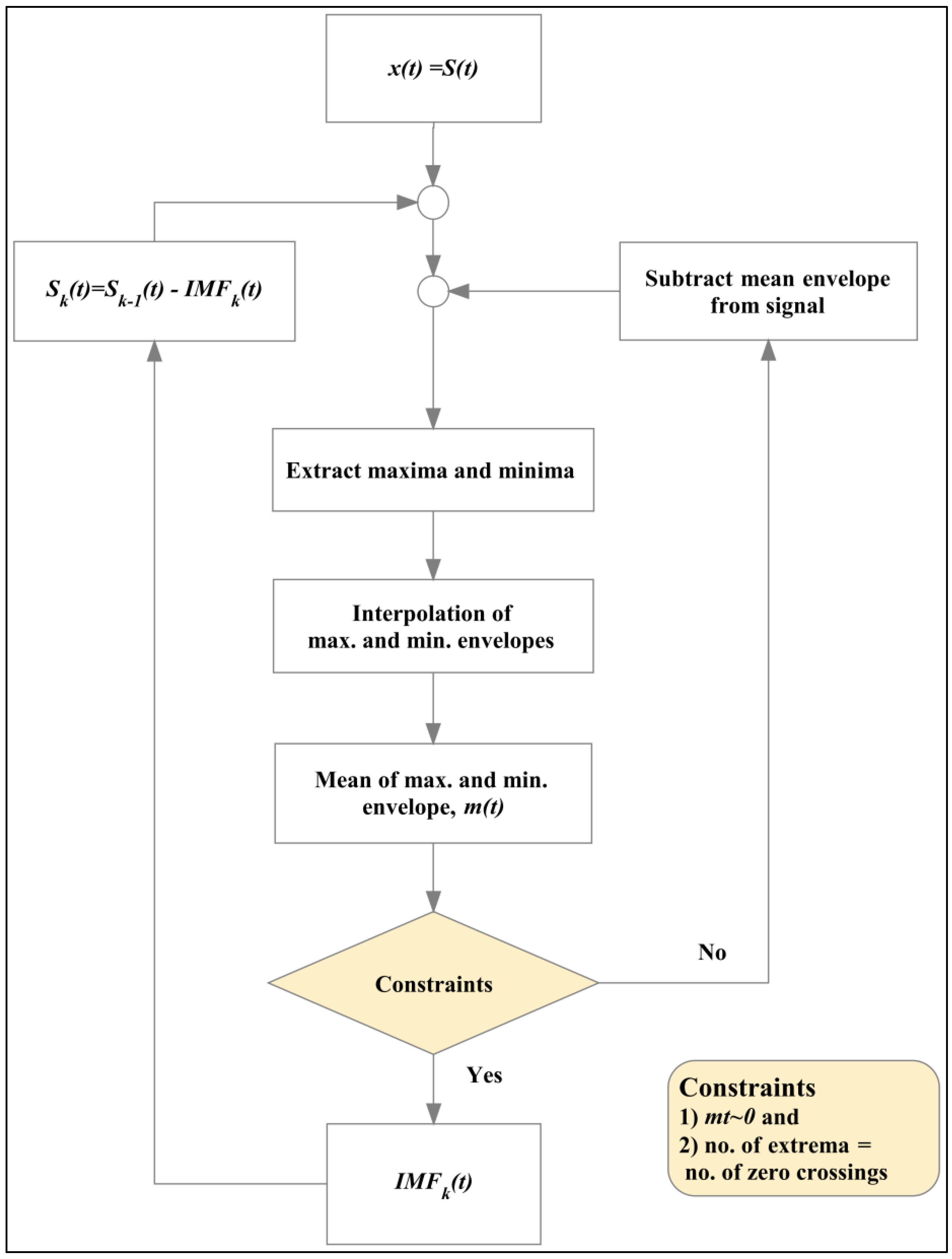
HHT is designed to decompose nonlinear and nonstationary signals, especially those with high volatility and fast frequency changes. The signal is adaptively decomposed into components and, after the decomposition of each step, the transformed signal is known as an Intrinsic Mode Function (IMF), which includes the different time scales intrinsic to the signal. IMF is a mono-component and can be transformed into an instantaneous frequency. IMF signals have also been defined as a function with a zero mean and with as many zero crossings as maxima or minima. The HHT process is divided into two parts: EMD and Hilbert Spectral Analysis (HSA). Figure 1 shows the EMD mechanism using a sifting process. It starts by identifying the maxima and minima points, extracting them, interpolating the maxima and minima envelopes, and computing the means of the local envelope.

Figure 1. Flowchart of Empirical Mode Decomposition (EMD) in the Hilbert-Huang transform (HHT).

Figure 1. Flowchart of Empirical Mode Decomposition (EMD) in the Hilbert-Huang transform (HHT).

A nonlinear and nonstationary time series dataset is denoted as x_i(t). The IMF, c_i(t) is defined under the conditions that: (i) The numbers of extrema (maxima plus minima) and zero crossings in the entire data series must either be equal to or differ by at most one; and (ii) At any point, the mean value of the envelope defined by the local maxima and that defined by the local minima, must be zero [10]. These conditions are met

$$\left[\begin{array}{l}n{U}_i(t)+n{L}_i(t)=n{Z}_i(t),\\ n{U}_i(t)+n{L}_i(t)=n{Z}_i(t)\pm 1\end{array}\right]$$

(1)

and

$$\left[\frac{U_i(t)+L_i(t)}{2}=0\right]$$

where nU_i(t), nL_i(t) and nZ_i(t), are the values of the maxima (upper peak), minima (lower peak) and zero crossing, of the EMD respectively. The EMD algorithm can be represented as follows.

Step 1: Spline the EMD datasets denoted to x_k(t) by interrelating using U_i(t) and L_i(t), which is given by

$$f_{\mathrm{int}}\left\{U_k(t),x_k(t)\right\}=U_{1\mathrm{int}}(t),U_{2\mathrm{int}}(t),U_{3\mathrm{int}}(t),\mathrm{....},U_{n\mathrm{int}}(t)$$

(2)

and

$$f_{\mathrm{int}}\left\{L_i(t),x_k(t)\right\}=L_{1\mathrm{int}}(t),L_{2\mathrm{int}}(t),L_{3\mathrm{int}}(t),\mathrm{....},L_{1\mathrm{int}}(t)$$

(3)

The algorithm used for parabolic interpolation can be described as follows.

(1)

When constructing the upper and lower envelopes, we calculate the parabola coefficients of ax² + bx + c using x(k − 1), x(k), (k + 1);

(2)

If the second-degree coefficient, a, equals zero, is x(k) is certainly not an extremum so the sliding window moves further on a discrete value of x(k);

(3)

If the first-degree coefficient, b, equals zero, x(k) is an extremum, either a maximum or minimum, depending on the sign. We then calculate the top of this parabola by introducing $t_{\text{top}}=\frac{-b}{2a}$; similarly, applying to the bottom part of the parabolic curves;

(4)

Repeat (2) and (3) and stop after executing x(k + n).

Step 2: Average the maxima and minima in order of the time series, which is represented as

$$m_i(t)=\frac{U_{1\mathrm{int}}+L_{1\mathrm{int}}}{2},\frac{U_{2\mathrm{int}}+L_{2\mathrm{int}}}{2},\frac{U_{3\mathrm{int}}+L_{3\mathrm{int}}}{2},\mathrm{...},\frac{U_{n\mathrm{int}}+L_{n\mathrm{int}}}{2}$$

(4)

Step 3: Subtract the x_i(t) from the average of the local extrema (maxima and minima) m_i(t) in order of the time series, and the new decomposed signal is

$$h_i(t)=x_k(t)-m_i(t)$$

(5)

Step 4: Repeat steps (i) through (iii) k times until $h_{1k}(t)$ equals c₁(t). Using Equation (5) where $h_{1(k-1)}(t)-m_{1k}=h_{1k}(t)$, we designate c₁(t) as the first IMF.

Step 5: Find other IMFs by calculating the first residual, which is given by

$$r_1(t)=x_k(t)-c_1(t)$$

(6)

We derive $c_2(t),c_3(t),c_4(t),\mathrm{...},c_n(t)$; thus, $r_1(t)$ is treated as a new dataset in the next loop, which is completes after obtaining c_n(t). This procedure is represented by

$$r_2(t)=r_1(t)-c_2(t)$$

(7)

            ……

$$r_n(t)=r_{n-1}(t)-c_n(t)$$

(8)

IMFs are narrowed band, zero-mean signals and the signal is decomposed into k IMFs by EMD, so each IMF is located in lower frequency regions in the time-frequency domain than the lagged signal. EMD can act as a dyadic filter bank for noise [16] and can be expressed as follows.

$$x(t)={\displaystyle \sum _{i=1}^n{r}_n(t)+r_n(t)}$$

(9)

Since HHT has formed forms another function, HSA, it can be used as a tool for the time-frequency analysis of nonlinear and nonstationary datasets to present the results as a time-frequency-energy distribution [12]. For a comprehensive explanation of the Hilbert transform, refer to Cohen [16]. Given a real signal x(t), the analytic signal z(t) is defined as

z(t) = x(t) + iy(t)

(10)

where y(t) is the Hilbert transform defined using the Cauchy principle value denoted by p.v. of x(t) such that

$$y(t)=H[x(t)]=p.v.{\displaystyle \underset{-\infty }{\overset{+\infty }{\int }}\frac{x(\tau )}{\text{π}(t-\tau )}}\text{d}\tau$$

(11)

We can define the complex signals, amplitude A(t) and phase ψ(t) as follows [8]

(12)

$$\psi (t)=\arg z(t)=\text{arctan}\frac{y(t)}{x(t)}$$

(13)

where the time-varying phase or instantaneous frequency ω(t) can be given as $\omega (t)=\frac{\text{d}\psi (t)}{\text{d}t}$.

From Equation (9), the original data is rearranged as follows:

$$x(t)=\mathrm{Re}{\displaystyle \sum _{i=1}^n{A}_i(t)\exp (j{\displaystyle \int {\omega }_i(t)\text{d}t)}}$$

(14)

where Re {.} denotes real part of the complex quantity.

Using Equation (14) and performing the Hilbert transform on each IMF c_n(t), the analytical data can be expressed in terms of the Hilbert amplitude and instantaneous frequency, as follows:

$$\overline{x}(t)={\displaystyle \sum _{i=1}^n{R}_i(t)\exp [j{\displaystyle \int {\omega }_i(t)\text{d}t]}}$$

(15)

As the HHT model comprises two main parts: EMD and HSA, the EMD process under a cubic spline and sifting technique decomposes the original signals into IMF. HSA calculates the instantaneous frequency using the Hilbert transform and analyses the entire time-varying instantaneous spectrum. It is crucial to mention that the analysis of the Hilbert spectrum is conducted to view the spectrum after the EMD process is finished.

2.2. Creating the aIMF Algorithm

Kaslovsky and Meyer [17] explained that a meaningful instantaneous frequency (IF) decomposed by the EMD algorithm must be nearly monochromatic, of which is a condition that is not guaranteed by the algorithm and fails to be met clearly when the signals is corrupted by noise. Several reports demonstrated that the EMD performance is likely to be sensitive and produces a large quantity of noise [12,18]. Moreover, the accuracy of HHT analysis suffers from several mathematical and numerical effects that require further studies. This is mainly because HHT signals emerged from EMD algorithm are not shift-invariant in times (stationary) and is likely be full narrow band [18]. To reduce noise, one of the solutions was to normalise the analytic signal prior to Hilbert transform [8,19]. There were many studies to improve the HHT algorithms, and those at least are; adoption of wavelet packet transform as the pre-processes to decompose the signals into a set of narrow-band signals prior to the application of the EMD [20,21], and an ensemble empirical mode decomposition (EEMD) which consists of shifting an ensemble of white-added noise signals and treats the mean as a final true result, using a windowed average. One of the publications of the EEMD was used to add noise to provide stoppage criteria for the EMD process [9]. Kaiser [22] mentioned that Fourier spectral analysis and its derivatives such as WT encountered with a limited time window width by sliding a predetermined window(s) along the time axis. Moreover, there is a trade-off between the time consumed in the window width and the frequency resolution, and this phenomenon has been considered by the uncertainty principle Heisenberg [21]. In the WT, the window width must be preselected and it is known as the primary or mother wavelet which is a prototype that provides less flexibility when handling datasets where the mean and variances are highly volatile.

It is imperative to restate that two conditions of EMD process defined in Section 2.1. However, with more iteration, the more residual r_n(t) becomes either over-distorted or a monochromatic function from which no further IMF can be decomposed [11]. The other study confirmed that the real complex quantity of all IMFs decomposed i.e., IMF1 to IMF7, which are in the amplitude-frequency domain, shifted to the lower region [19].

To reduce noise produced in the EMD process, we propose to extract noise spreading to all of the spectrums by averaging all IMFs and subtract them from the original signals in which is represented by

$$c_a(t)=\frac{{\displaystyle \sum _{i=1}^n{c}_i(t)}}{n}$$

(16)

Next, we subtract the averaged IMF in Equation (16), c_a(t), from the original nonlinear, nonstationary times series datasets, x_n(t). Thus, a new digital filter is created, which is given by

$$\text{aIMF}(t)=y_n(t)=x_i(t)-c_a(t)$$

(17)

where y_n(t) is a function of the aIMF algorithm.

In Figure 2, the aIMF process starts by inputting the nonlinear, nonstationary times series data, Euro and US dollars (EUR-USD), exchange rates into the EMD process. The next block uses the results from the EMD process whereas the aIMF algorithm begins in the third block where all of the IMFs are averaged and the averaged IMFs are subtracted from the original datasets.

Figure 2. Block diagram of the proposed averaging Intrinsic Mode Function (aIMF) algorithm.

Figure 2. Block diagram of the proposed averaging Intrinsic Mode Function (aIMF) algorithm.

Referring to Figure 2, the proposed algorithm aIMF has an advantage which provides stoppage criteria once the two conditions of the EMD process defined in Section 2.1 are accomplished. This is because with more iteration, the more residual r_n(t) becomes either over-distorted or a monochromatic function from which no further IMF can be decomposed.

2.3. Theoretical Considerations of the WT Algorithm

Helong et al. [23] applied the WT of a signal f(x), which was early defined in [21] as follows

$$WT(a,b;x,\psi )={\left|a\right|}^{-\raisebox{1ex}{$1$}\!\left/ \!\raisebox{-1ex}{$2$}\right.}{\displaystyle \underset{-a}{\overset{+\infty }{\int }}f(x)\psi \overline{\left(\frac{x-b}{a}\right)}}\text{d}x$$

(18)

where WT represents the calculated coefficients, and b are the translation parameters and scale, respectively, ψ(x) is the transforming function (mother wavelet) and the bar over ψ indicates its complex conjugate. A wavelet is classified as an adaptive algorithm, which is used in many fields such as astronomy, acoustics, nuclear engineering, signal processing and the prediction of earthquakes by solving partial optimized equations and reducing the random noise [15]. A factorization of f at different resolution levels is defined by

$$f={\displaystyle \sum _{i=-\infty }^{+\infty }{c}_{J,i}{\varphi }_{J,i}+{\displaystyle \sum _{j=J}^1{\displaystyle \sum _{i=-\infty }^{+\infty }{d}_{j,i}{\psi }_{j,i}}}}$$

(19)

where C_J,i represents the information in the signal on the coarsest level, ϕ_J,i is the scaling function and d_J,i represents the details (wavelet coefficients) at the different scales necessary to reconstruct the function at the fine scale 0, at which the wavelet and scaling functions are compactly supported.

The next step is to introduce the thresholding technique that is used to remove noise from each local set of d_J,i, which are normally affected at different levels of the scale j. This is given by Li [24]

$$\gamma =\{\begin{array}{cc}{d}_i-\lambda & d_i\succ \lambda \\ 0& \Vert d_i\Vert \le \lambda \\ d_i+\lambda & d_i\prec -\lambda \end{array}$$

where γ is the indicator and λ is the thresholding value. To find the thresholding value λ, we introduce factorizing f and we obtain $\widehat{f}$, which approximates f. The error (risk) between f and its approximation $\widehat{f}$ is given by

$$R\left(\widehat{f},f\right)=\frac{1}{N}{{\displaystyle \sum _{i=0}^{N-1}\Vert {\widehat{f}}_i-f_i\Vert }}_2^2$$

(20)

In terms of the wavelet coefficients under Parseval’s identity [24], the transform shown in Equation (20) can be expressed as

$$R\left(\widehat{f},f\right)\propto {\Vert d-d\Vert }_2^2={\displaystyle \sum _j{\displaystyle \sum _k({\widehat{d}}_{j,k}-d_{j,k}}}{)}^2$$

(21)

Applying Equations (19) and (21) with respect to any resolution level, j = 1, 2, ..., J, we use Stein’s principle [25] to minimize the risk in Equation (21). The thresholding value λ is finally obtained as

$$\lambda =2\sqrt{\frac{1}{N}{\displaystyle \sum _j{\displaystyle \sum _k({\widehat{d}}_{j,k}-d_{j,k}}}{)}^2}$$

(22)

2.4. Theoretical Considerations of the EKF Algorithm

In a nonlinear system, however, KF can be enhanced using a Taylor series to expand the state Equation (23) and output Equation (24) around a nominal state, known as a linearized KF. A summary of the linearized KF algorithm is

x_k+1 = f(x_k,u_k) + w_k

(23)

y_k = h(x_k) + v_k

(24)

where x_k+1 is the state of the system, denoted for the next time series of the original datasets x_k; k is the time index; u_k is the driving function that may call a signal control or distribution function; w_k is a noise, independent and identically distributed (i.i.d.) N(0,Q), where Q is the covariance (matrix) of the state; v_k and is another noise, i.i.d. N(0,R), where R is the covariance (matrix) of the measurement of noise; y_k is the measured output; and f(.) and h(.) are the state equation and output equation, respectively. The state and output functions in the case are nonlinear functions. Thus, Equations (27) and (28) are nominal states that are known (predicted) ahead of time, which are represented by

(25)

(26)

where ${\overline{x}}_{k+1}$ is the nominal state of the system and y is the nominal measured output state.

During each step, we compute the partial derivative matrices of A_k and C_k with respect to x_k, and we obtain in the following equations

(27)

(28)

where A and C are matrices. Next, we define Δy_k as the difference between the actual measurement y_k and the nominal measurement y_k, which is given by

$$\Delta y_k=y_k-{\overline{y}}_k=y_k-h({\overline{x}}_k)$$

(29)

In this state, the following linearized KF equations can be executed as follows:

(30)

$$\text{Δ}{\widehat{x}}_{k+1}=A_k\text{Δ}{\widehat{x}}_k+K_k(\text{Δ}{y}_k-C_K\text{Δ}{\widehat{x}}_k)$$

(31)

(32)

$${\widehat{x}}_{k+1}={\overline{x}}_{k+1}+\text{Δ}{\widehat{x}}_{k+1}$$

(33)

where K_k is the Kalman gain, P_k is the covariance of the error of the estimation and I is the identity matrix.

In the linearized KF, there is a limitation that the nominal state x must be set prior the execution. EKF then assumes that x equals $\widehat{x}$ in the bootstrapping approach to the state equation. Thus, Equations (27) and (28) are subsequently changed to

(34)

$$C_k=h^{\prime }({\widehat{x}}_k)$$

(35)

In Equation (31), where x equals $\widehat{x}$ , Equation (31) can be rearranged to produce

(36)

substitute Equations (34) and (35) into Equation (36), we obtain Equation (37). As a result, EKF equation can be represented by applying Equations (31), (32) and (37) which is given by

$${\widehat{x}}_{k+1}=f({\widehat{x}}_k,u_k)+K_k[y_k-h({\widehat{x}}_k)]$$

(37)

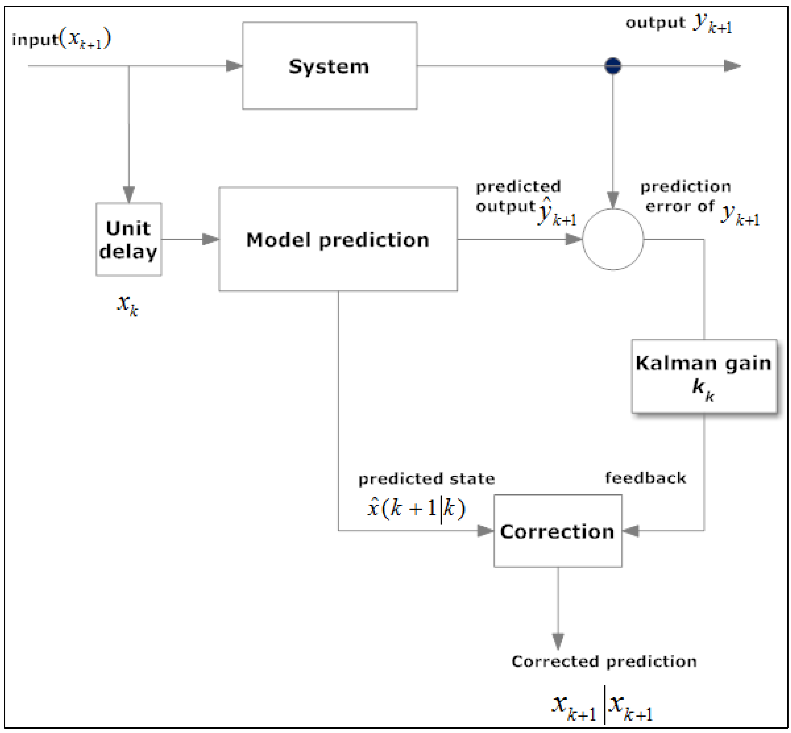
In the initial state where k = 0, x is predetermined using its means and Q_k and R_k are relevant to x. In the execution mode, the measurement update (output state) adjusts the projected estimate based on an actual measurement at that time. It should be noted that EKF applies Equations (30), (31) and (37) to update the prediction mode after the state is changed periodically and the Kalman gain K_k determines how the observer responds to the difference between its estimated output and the noisy measurement. To simplify this, we can present EKF as the system block diagram shown in Figure 3.

Figure 3. System block diagram of Extended Kalman Filter (EKF).

Figure 3. System block diagram of Extended Kalman Filter (EKF).

2.5. Theoretical Considerations of the PF Algorithm

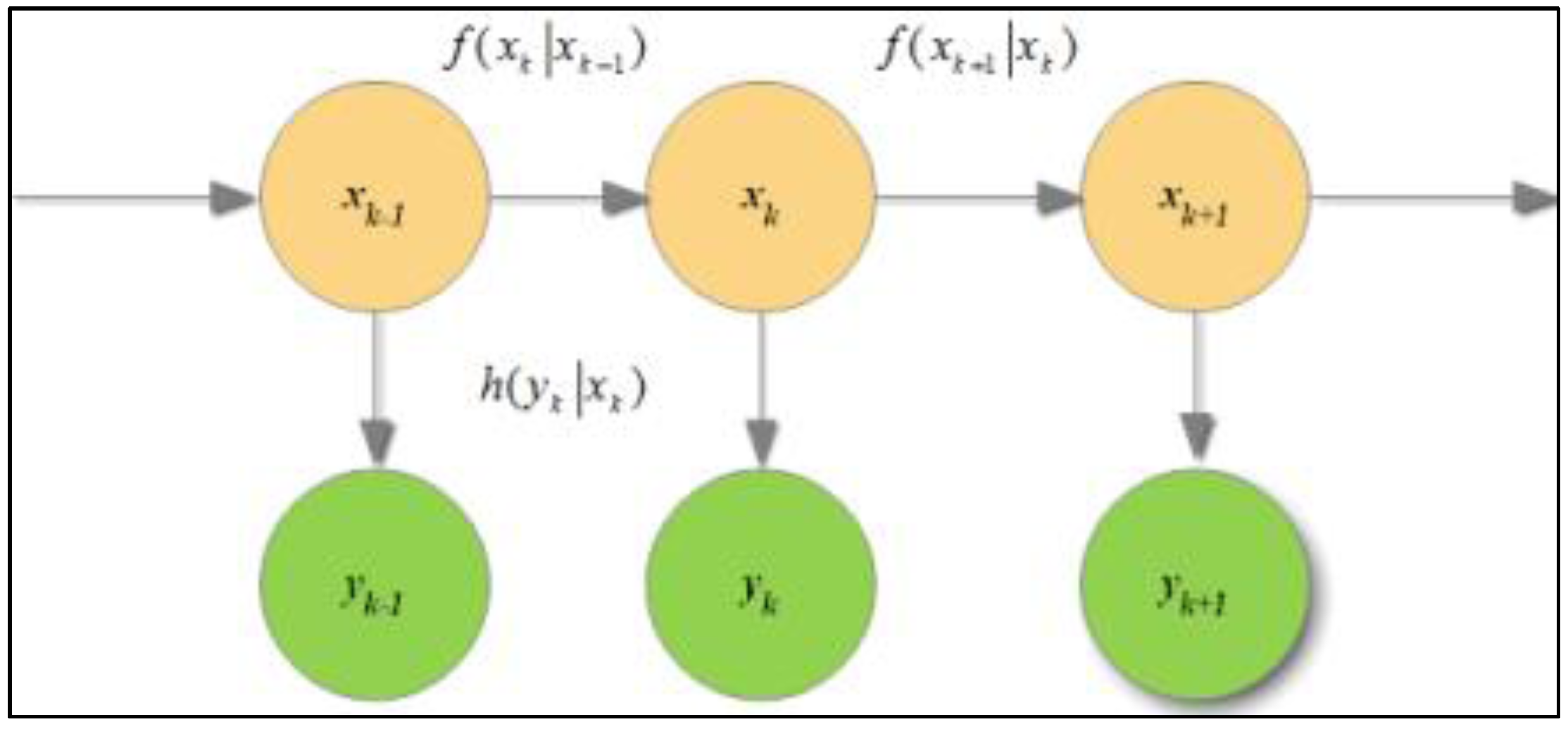
The theoretical considerations of the PF model start by considering a hidden Markov model (HMM) that observes the outputs x_i indirectly using state y_i, and we can specify a simple model as follows

$$x_1~\mu \left(x_1\right)$$

(38)

$$f(x_k|x_{k-1})$$

(39)

where in state equation (transition) for k > 1, and

$$h(y_k|x_k) \text{in measured state }\left(\text{observation}\right)$$

(40)

where all states are homogeneous, and the probabilities of transitions and observations are independent of time, see Figure 4.

Figure 4. HMM showing the transition and observation states.

Figure 4. HMM showing the transition and observation states.

The goal is to estimate x_k, which is equivalent to x_i the original datasets, given all observations up to point (y_1:n). Alternatively, we need to find the posterior distribution of p(x_1:n|y_1:n). Using Bayes, we end up with two steps as follows:

(i)

Update step:

$$p(x_k|y_{1:k})=\frac{h(y_k|x_k)p(x_k|y_{1:k-1})}{p(y_k|y_{1:k-1})}$$

(41)

(ii)

Prediction step:

$$p(x_k|y_{1:k-1})={\displaystyle \int f(x_k}|x_{k-1})p(x_{k-1}|y_{1:k-1})d{x}_{k-1}$$

(42)

We often find that these distributions were intractable, especially the nonlinear and Gaussian model in closed form. The solution is to approximate the distributions using a large number of samples (particles). To address the problems in Equations (41) and (42), it might not be too difficult to appropriate the intractable integrals appearing in those equations directly, where the alternative is to use important sampling or sequential importance sampling (SIS). The advantage of SIS is that it does not guarantee to fail as t increases and it becomes more and more skewed, especially when sampling high-dimensional spaces [26].

Thus, we propose a bootstrap PF, which is an iterative method of Bayesian inference for a dynamic state space. The algorithm of the bootstrap PF model is described as follows:

(1)

Assume $p(x_{k-1}|y_{k-1})$ is the posterior probability distribution at k − 1 where the transition state (state equation) is

(2)

Resample $p(x_k|x_{k-1})$, which is the prior probability distribution at k − 1 using the bootstrap algorithm

(3)

Find a weight by Monte Carlo integration using $p(x_{k-1}|y_{k-1})$ and $p(x_k$ to obtain, ${\displaystyle \int p\left(x_k|x_{k-1}\right)\cdot p\left(x_{k-1}|y_{k-1}\right)\text{d}{x}_{k-1}}\approx {\displaystyle \sum _i{w}_{k-1}^i}p\left(x_k|x_{k-1}^i\right)$

(4)

From (3), use to estimate the particle at k − 1 and obtain ${\widehat{S}}_{k-1}=\left\{({\widehat{x}}_{k-1}^i,{\widehat{w}}_{k-1}^i);i=1,2,\mathrm{...},N\right\}$.

(5)

Update the likelihood function $p(y_k$ with ${\hat{x}}_{k-1}^i$ and ${\hat{w}}_{k-1}^i$.

(6)

From (5) use the new updated likelihood to update $p(x_k$, which is the posterior probability distribution at k using a normalised weight from time to time. The weight can either be the averaging of all the weights or the last weight only.

(7)

Finally, we obtain $p(x_k|y_k)$ the posterior probability distribution at k.

3. Simulation and Results

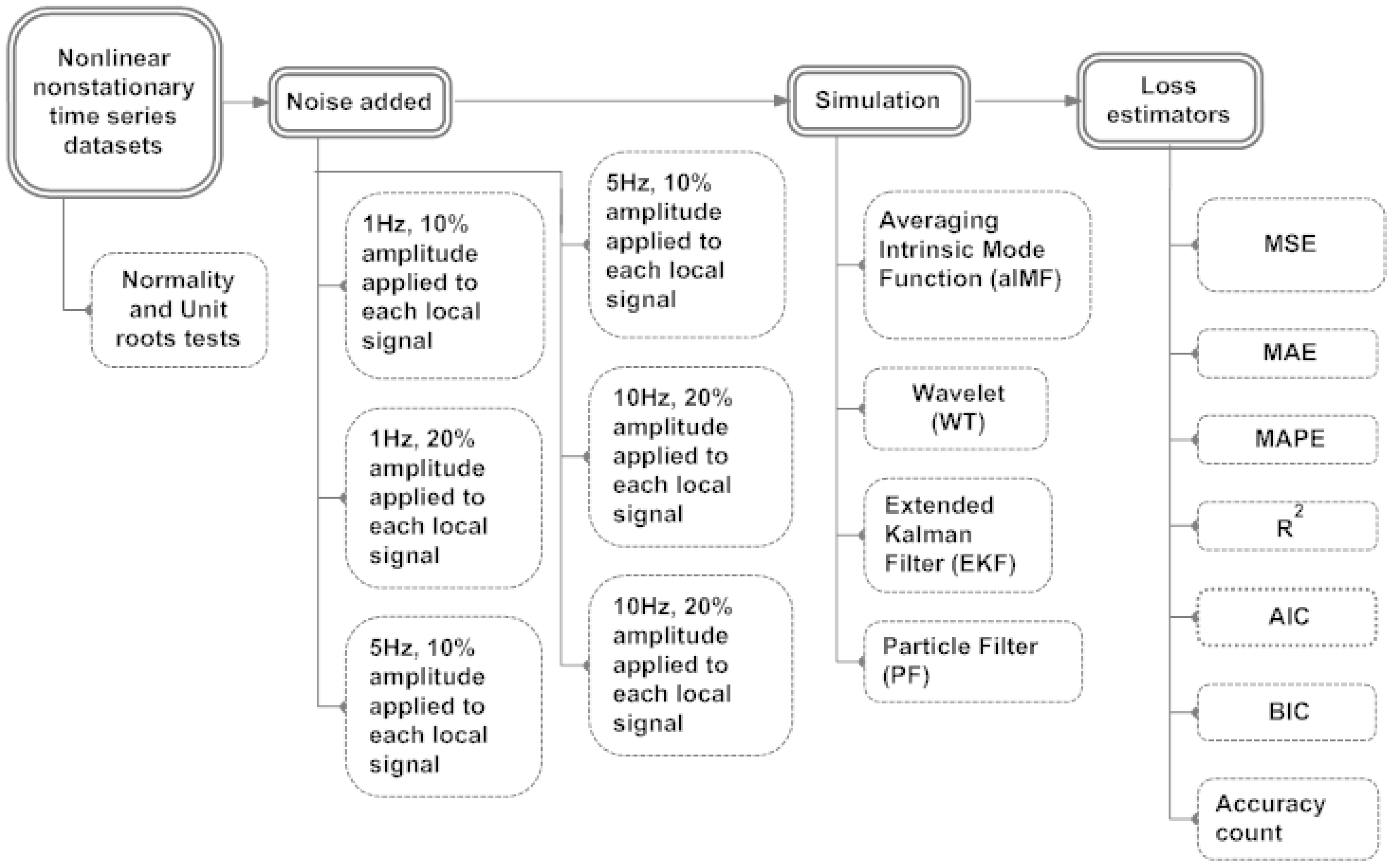
The aim of this section is to compare the performances of all the proposed digital filters and recommend the best fit filter. We use R Programming to simulate the original datasets that has a suite of noise added to it. After completing the simulations, we applied a variety of loss estimations, i.e., Mean Square Error (MSE), Mean Absolute Error (MAE), Mean Absolute Percentage Error (MAPE), R², AIC, BIC and Accuracy count which is a sum of the upward and downward movements of all the underlying local signals after they had transited the reversion points. See flowchart of simulation and results in Figure 5.

Figure 5. Flowchart shows simulation and results of aIMF, WT, EKF and PF.

Figure 5. Flowchart shows simulation and results of aIMF, WT, EKF and PF.

3.1. Adding White-Gaussian Noise

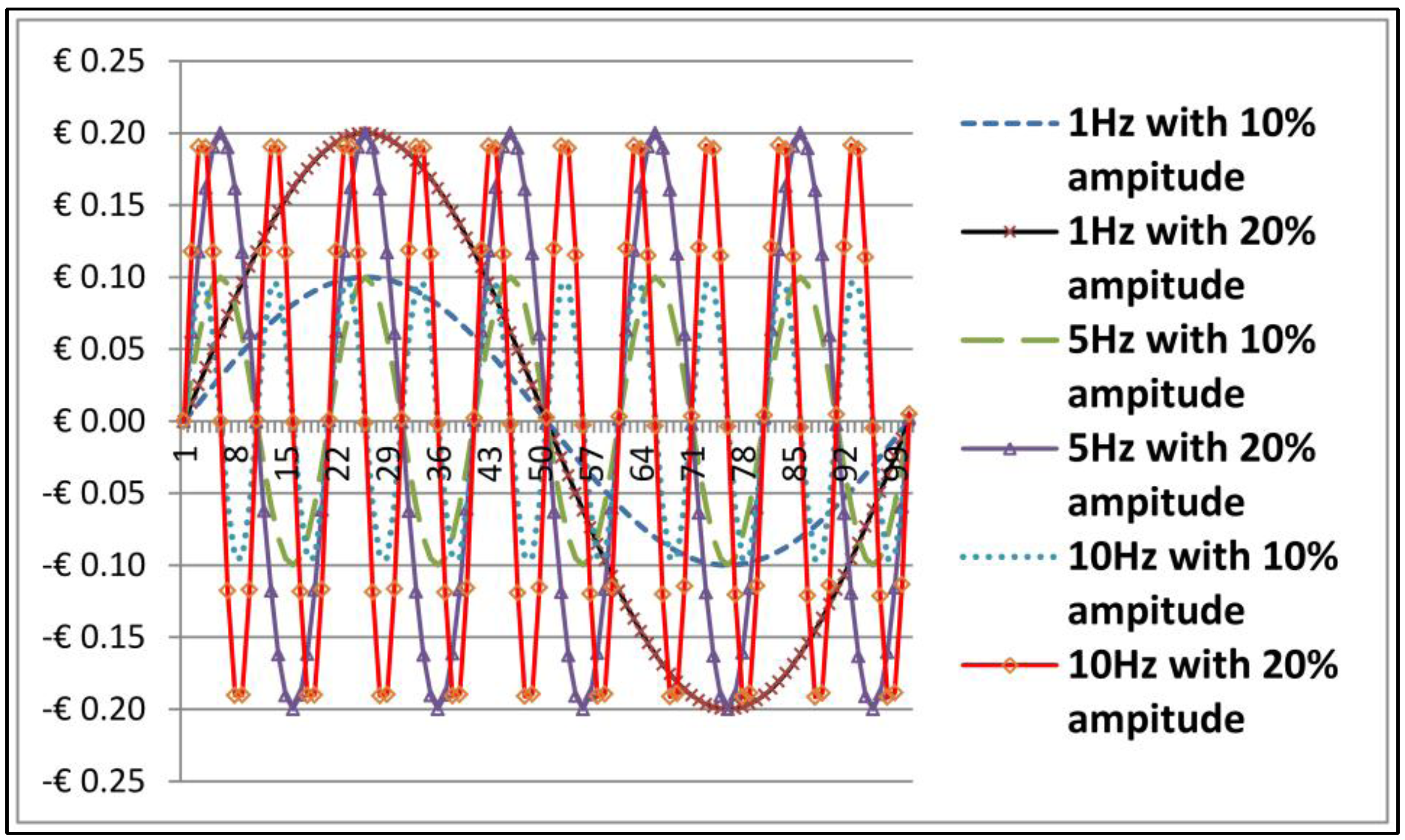
We created six sets of sine wave which is i.i.d. N(0,${\sigma }^2$) for the frequencies in Hz of 1, 5 and 10 with the amplitude of 10% and 20% of the original datasets, at 100% random distribution. Those parameters were applied to the exchange rates data points x_k(t) in time series. The distribution of these added noise are similar to white-Gaussian noise as shown in Figure 6.

Figure 6. Six sets of sine wave as frequencies in Hz of 1, 5 and 10 with the amplitude of 10% and 20% of exchange rates.

Figure 6. Six sets of sine wave as frequencies in Hz of 1, 5 and 10 with the amplitude of 10% and 20% of exchange rates.

For ease of presentation, Figure 6 shows the x-axis representing just 100 data points out of the total 2322 data points in the time series, whereas the y-axis is representing the amplitude. We introduced a variety of testing methods, namely; (a) Anderson-Darling, Lilliefors (Kolmogorov-Smirnov) and Pearson chi-square for nonlinear test; and (b) Augmented Dickey-Fuller and Elliott-Rothenberg-Stock for nonstationary test. Referring to Equation (23) x_k represented datasets, EUR-USD, exchange rates, in which their nonlinear and nonstationary characteristics were verified by all the testing methods; and w_k represented the six sets of sine wave created in Section 3.1. The equation which used to add white Gaussian noise to the original datasets can be rearranged as follows

$$x_{kg}(t)=x_k(t)+{\epsilon }_{kg}(t)$$

(43)

where x_kg(t) is the original signal with the noise, x_k(t) is the original datasets and ${\epsilon }_{kg}(t)$ is the added noise with i.i.d. N(0,1) at section of various frequencies in Hz of 1, 5 and 10 with 100% of random distribution of x_k(t). To verify that the Equation (43) is nonlinear equation, we tested the x_kg(t) with the different parameters of the noise added. As per the results, all of the p-value generated by all the testing methods mentioned earlier were less than 0.05. This served to imply that the characteristics of x_kg(t) was nonlinear and nonstationary. Later, x_kg(t) was used as input signal to estimate the performance of the following algorithms: (i) aIMF, (ii) WT, (iii) EKF and (iv) PF.

3.2. Simulation and Performance Measurements of the aIMF Algorithm

The objective of this section is to measure the performance of the aIMF algorithm compared with the original datasets, i.e., the EUR-USD exchange rates. To test the performance of the proposed aIMF algorithm when filtering the original signals with white Gaussian noise, we applied a variety of loss estimators, i.e., MSE, MAE, MAPE, R² and Accuracy count.

At the beginning, we tested the five exchange rates i.e., EUR-USD with Normality and Unit Root tests and found that they are nonlinear and nonstationary time series. Next, we simulated the aIMF algorithm using an R Programming that comprised C++ scripts, which followed the logic in Section 2.2. Figure 7 shows that we produced a new signal, which was filtered by the aIMF algorithm.

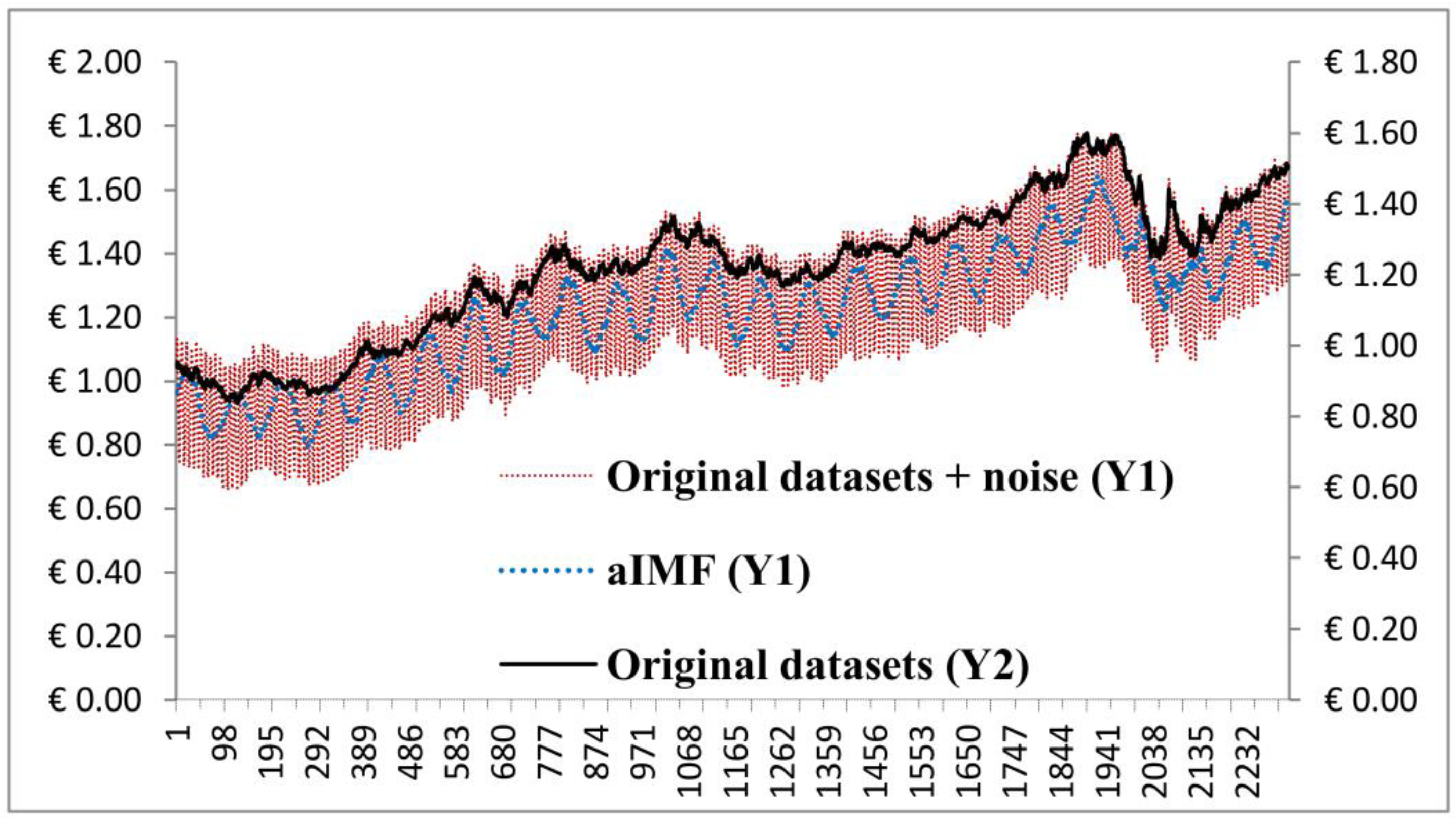
Figure 7. Plots of the original datasets, original datasets + noise, and the aIMF algorithm.

Figure 7. Plots of the original datasets, original datasets + noise, and the aIMF algorithm.

Having simulated the aIMF algorithm with all noise parameters mentioned in the early of Section 3.1, the results are in the same magnitude and directions. To simplify the graph presentation, we selected the x-axis representing the data points in the time series of overall data range, and two sets of y-axis representing the original datasets, EUR-USD exchange rates (Y2) and the original datasets + noise (Y1) of which shows only the noise’s plot of 1 Hz at 10% amplitude (Y1) with 100% random distribution. We analysed the plots and found that the aIMF curve resided within the curve of “the original datasets + noise”. The trend of those three plots was in the same direction. In terms of estimation, Table 1, Table 2, Table 3, Table 4, Table 5 and Table 6 indicate that all loss estimators, namely; MSE, MAE, and MAPE are relatively low ranging from 0.00296–0.00596, 0.04838–0.06618 and 4.08815–5.59678, respectively.

The R² is in the high ranging, from 0.8533–0.9228, whereas, AIC and BIC are high, up to −6305.47 and −6974.09, respectively. The Accuracy count showed 57.69%–79.66%. As a result, the performance of the aIMF is acceptable.

We continued the simulations using 5% of random distribution of the added noise instead of 100%. The results showed that the less numbers of the random noise distributed the better performance of the aIMF algorithm. For example, at 5% random distribution of the added noise at 1 Hz with 10% amplitude, the loss estimators, namely; MSE, MAE, MAPE, R², AIC, BIC and Accuracy count were 0.00014, 0.01019, 0.88981, 0.99820, −15723.93, −15706.68, and 95.86%, respectively; and it outperformed those of simulations with 100% random distribution.

Table 1. Performance measurements of original datasets using noise distribution at 100% with 1 Hz and 10% amplitude of the original signals.

EUR-USD	MSE	MAE	MAPE	R2	AIC	BIC	Accuracy count (%)
aIMF	0.00399	0.05636	4.77093	0.8962	−6305.47	−6288.22	77.34
WT	0.00506	0.05402	5.54677	0.7231	−6877.81	−7857.63	53.82
EKF	0.00548	0.06432	5.44475	0.8701	−5783.21	−5765.96	47.13
PF	4.52658	1.65756	140.015	0.0062	−1060.50	−1043.25	50.32

Table 1. Performance measurements of original datasets using noise distribution at 100% with 1 Hz and 10% amplitude of the original signals.

EUR-USD	MSE	MAE	MAPE	R2	AIC	BIC	Accuracy count (%)
aIMF	0.00399	0.05636	4.77093	0.8962	−6305.47	−6288.22	77.34
WT	0.00506	0.05402	5.54677	0.7231	−6877.81	−7857.63	53.82
EKF	0.00548	0.06432	5.44475	0.8701	−5783.21	−5765.96	47.13
PF	4.52658	1.65756	140.015	0.0062	−1060.50	−1043.25	50.32

Table 2. Performance measurements of original datasets using noise distribution at 100% with 1 Hz and 20% amplitude of the original signals.

EUR-USD	MSE	MAE	MAPE	R2	AIC	BIC	Accuracy count (%)
aIMF	0.00296	0.04838	4.08815	0.9228	−6991.34	−6974.09	79.66
WT	0.05439	0.05311	5.79178	0.6759	−6397.83	−6804.50	54.23
EKF	0.02043	0.12765	10.7989	0.6385	−3407.66	−3390.41	48.51
PF	4.43079	1.64779	139.747	0.0067	−1061.73	−1044.48	49.76

Table 2. Performance measurements of original datasets using noise distribution at 100% with 1 Hz and 20% amplitude of the original signals.

EUR-USD	MSE	MAE	MAPE	R2	AIC	BIC	Accuracy count (%)
aIMF	0.00296	0.04838	4.08815	0.9228	−6991.34	−6974.09	79.66
WT	0.05439	0.05311	5.79178	0.6759	−6397.83	−6804.50	54.23
EKF	0.02043	0.12765	10.7989	0.6385	−3407.66	−3390.41	48.51
PF	4.43079	1.64779	139.747	0.0067	−1061.73	−1044.48	49.76

Table 3. Performance measurements of original datasets using noise distribution at 100% with 5 Hz and 10% amplitude of the original signals.

EUR-USD	MSE	MAE	MAPE	R2	AIC	BIC	Accuracy count (%)
aIMF	0.00522	0.06303	5.32770	0.8760	−5891.33	−5874.08	74.92
WT	0.00599	0.05636	4.77151	0.8962	−6303.39	−6286.15	55.51
EKF	0.00503	0.06159	5.22073	0.8807	−5980.49	−5963.24	47.65
PF	4.47322	1.64897	139.488	0.0096	−1067.39	−1050.14	50.24

Table 3. Performance measurements of original datasets using noise distribution at 100% with 5 Hz and 10% amplitude of the original signals.

EUR-USD	MSE	MAE	MAPE	R2	AIC	BIC	Accuracy count (%)
aIMF	0.00522	0.06303	5.32770	0.8760	−5891.33	−5874.08	74.92
WT	0.00599	0.05636	4.77151	0.8962	−6303.39	−6286.15	55.51
EKF	0.00503	0.06159	5.22073	0.8807	−5980.49	−5963.24	47.65
PF	4.47322	1.64897	139.488	0.0096	−1067.39	−1050.14	50.24

Table 4. Performance measurements of original datasets using noise distribution at 100% with 5 Hz and 20% amplitude of the original signals.

EUR-USD	MSE	MAE	MAPE	R2	AIC	BIC	Accuracy count (%)
aIMF	0.00596	0.06415	5.42792	0.8534	−5501.99	−5484.74	64.41
WT	0.00571	0.07660	4.78754	0.8761	−6890.19	−6897.21	56.13
EKF	0.01870	0.12247	10.3683	0.6637	−3575.62	−3558.38	48.00
PF	4.50770	1.64377	138.983	0.0074	−1063.27	−1046.02	50.58

Table 4. Performance measurements of original datasets using noise distribution at 100% with 5 Hz and 20% amplitude of the original signals.

EUR-USD	MSE	MAE	MAPE	R2	AIC	BIC	Accuracy count (%)
aIMF	0.00596	0.06415	5.42792	0.8534	−5501.99	−5484.74	64.41
WT	0.00571	0.07660	4.78754	0.8761	−6890.19	−6897.21	56.13
EKF	0.01870	0.12247	10.3683	0.6637	−3575.62	−3558.38	48.00
PF	4.50770	1.64377	138.983	0.0074	−1063.27	−1046.02	50.58

Table 5. Performance measurements of original datasets using noise distribution at 100% with 10 Hz and 10% amplitude of the original signals.

EUR-USD	MSE	MAE	MAPE	R2	AIC	BIC	Accuracy count (%)
aIMF	0.00527	0.06444	5.44396	0.8710	−5799.61	−5782.36	67.26
WT	0.00508	0.06890	5.79883	0.8948	−6273.51	−6745.29	56.82
EKF	0.00406	0.05546	4.69540	0.9017	−6429.89	−6412.64	51.66
PF	4.47322	1.64897	139.487	0.0096	−1067.39	−1050.14	50.24

Table 5. Performance measurements of original datasets using noise distribution at 100% with 10 Hz and 10% amplitude of the original signals.

EUR-USD	MSE	MAE	MAPE	R2	AIC	BIC	Accuracy count (%)
aIMF	0.00527	0.06444	5.44396	0.8710	−5799.61	−5782.36	67.26
WT	0.00508	0.06890	5.79883	0.8948	−6273.51	−6745.29	56.82
EKF	0.00406	0.05546	4.69540	0.9017	−6429.89	−6412.64	51.66
PF	4.47322	1.64897	139.487	0.0096	−1067.39	−1050.14	50.24

Table 6. Performance measurements of original datasets using noise distribution at 100% with 10 Hz and 20% amplitude of the original signals.

EUR-USD	MSE	MAE	MAPE	R2	AIC	BIC	Accuracy count (%)
aIMF	0.00580	0.06618	5.59678	0.8533	−5501.09	−5483.84	57.69
WT	0.00521	0.06003	4.57416	0.6941	−6843.56	−6899.78	53.34
EKF	0.01490	0.11046	9.34639	0.7140	−3951.51	−3934.26	51.62
PF	4.61609	1.67868	141.868	0.0049	−1057.44	−1040.19	50.45

Table 6. Performance measurements of original datasets using noise distribution at 100% with 10 Hz and 20% amplitude of the original signals.

EUR-USD	MSE	MAE	MAPE	R2	AIC	BIC	Accuracy count (%)
aIMF	0.00580	0.06618	5.59678	0.8533	−5501.09	−5483.84	57.69
WT	0.00521	0.06003	4.57416	0.6941	−6843.56	−6899.78	53.34
EKF	0.01490	0.11046	9.34639	0.7140	−3951.51	−3934.26	51.62
PF	4.61609	1.67868	141.868	0.0049	−1057.44	−1040.19	50.45

3.3. Simulation and Performance Measurements of the WT Algorithm

The objective of this section was to measure the performance of the WT algorithm compared with the original datasets, i.e., the EUR-USD exchange rates using the same simulating model and loss estimators employed in Section 3.2.

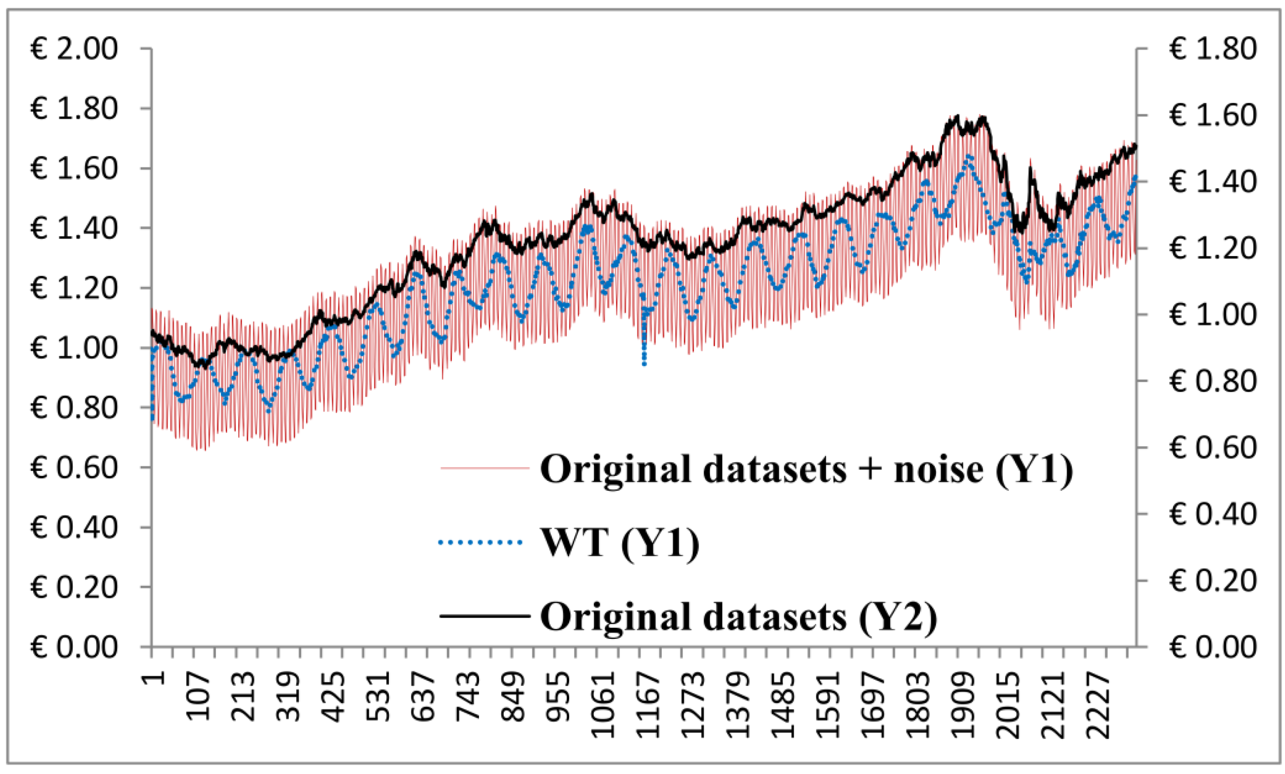
Similar to Figure 7, Figure 8 shows three plots, i.e., the original datasets (Y2), the “original datasets + noise” (Y1) and “WT” (Y1). We analysed the plots and found that the WT curve resided within the curve of “the original datasets + noise” except a spike occurred at between the data 1112nd to 1213rd rank of the x-axis. The trend of those three plots was in the same direction. In terms of estimation, Table 1, Table 2, Table 3, Table 4, Table 5 and Table 6 indicate that all loss estimators, namely; MSE, MAE, MAPE are relatively low, ranging from 0.00506–0.00599, 0.05402–0.07660 and 4.7715–5.79883, respectively. The R² is in the below standard ranging from 0.85340–0.8948, whereas, AIC and BIC are relatively high, up to −6890.19 and −6286.15, respectively; whereas the Accuracy counts showed 53.82%–56.13%. As a result, we rated the performance of the WT algorithm is relatively low and hardly acceptable.

Figure 8. Plots of the original datasets, original datasets + noise, and the Wavelet Transform (WT) algorithm.

Figure 8. Plots of the original datasets, original datasets + noise, and the Wavelet Transform (WT) algorithm.

3.4. Simulation and Performance Measurements of the EKF Algorithm

The objective of this section is to measure the performance of the EKF algorithm compared with the original datasets, i.e., the EUR-USD exchange rates using the same methods employed by Section 3.2.

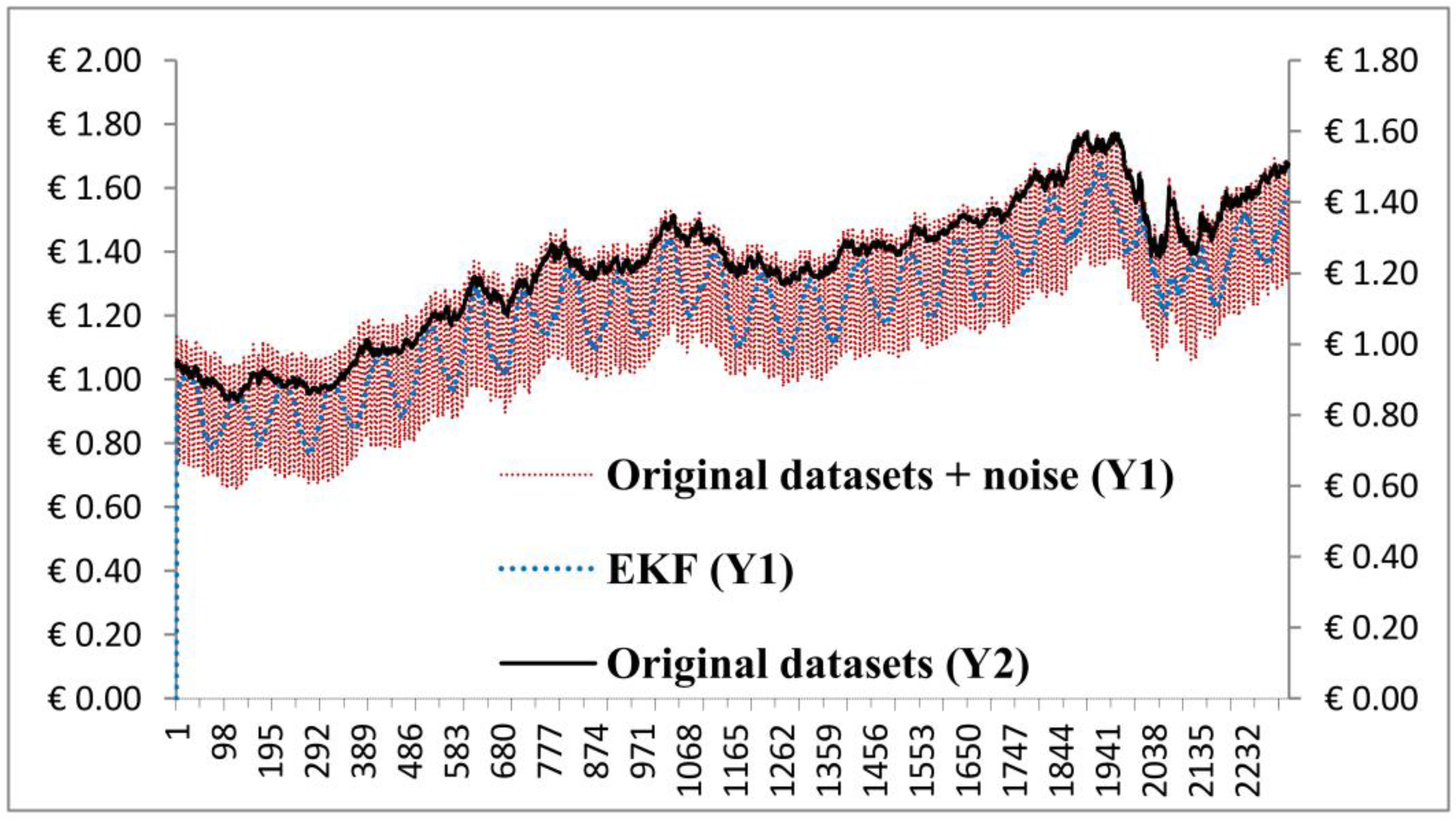
Similar to Figure 7, Figure 9 shows three plots, i.e., the original datasets (Y2), the “original datasets + noise” (Y1) and EKF (Y1). We analysed the plots and found that the EKF curve resided within the curve of “the original datasets + noise” except a spike occurred at the beginning of the x-axis. The trend of those three plots was in the same direction. In terms of estimation, Table 1, Table 2, Table 3, Table 4, Table 5 and Table 6 indicate that all loss estimators, namely; MSE, MAE, MAPE are relatively low ranging from 0.00406–0.01870, 0.05546–0.12765 and 4.69540–10.7989, respectively. The R² is in the ranging from 0.6637–0.9017, whereas, AIC and BIC are high, up to −6429.89 and −6412.64, respectively, and the Accuracy count showed 47.13%–51.66%. As a result, the performance of the EKF algorithm is unacceptable.

Figure 9. Plots of the original datasets, original datasets + noise, and the EKF algorithm.

Figure 9. Plots of the original datasets, original datasets + noise, and the EKF algorithm.

3.5. Simulation and Performance Measurements of the PF Algorithm

The objective of this section is to measure the performance of the PF algorithm compared with the original datasets, i.e., the EUR-USD exchange rate using the same methods employed by Section 3.2.

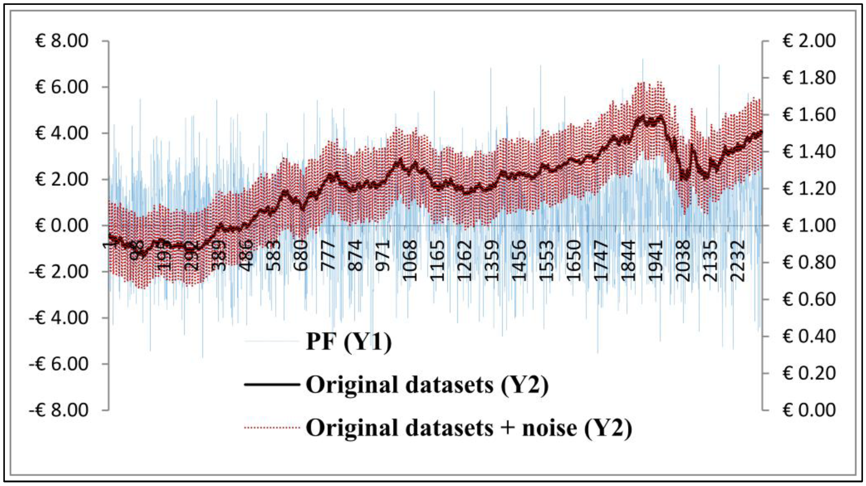
Similar to Figure 7, Figure 10 shows three plots, i.e., the original datasets (Y2), the “original datasets + noise” (Y2) and PF (Y1). We analysed the plots and found that the PF curve did not agree with the curve of “the original datasets + noise” and the original dataset’s, inasmuch as fluctuations of those three plots were not the same. The loss estimations emerged by varieties of noise parameters, in terms of estimation, Table 1, Table 2, Table 3, Table 4, Table 5 and Table 6 indicate that all loss estimators, namely; MSE, MAE, MAPE are relatively low ranging from 4.43079–4.52658, 1.64377–1.67868 and 139.488–141.868, respectively. The R² is unacceptable with the ranging of 0.0049–0.096, whereas, AIC and BIC are relatively too low i.e., −1067.39 and −1046.02, respectively, whereas the Accuracy count showed 49.76%–50.58%. As a result, the performance of the PF algorithm is also unacceptable.

Figure 10. Plots of the original datasets, original datasets + noise, and the Particle Filter (PF) algorithm.

Figure 10. Plots of the original datasets, original datasets + noise, and the Particle Filter (PF) algorithm.

3.6. Discussion

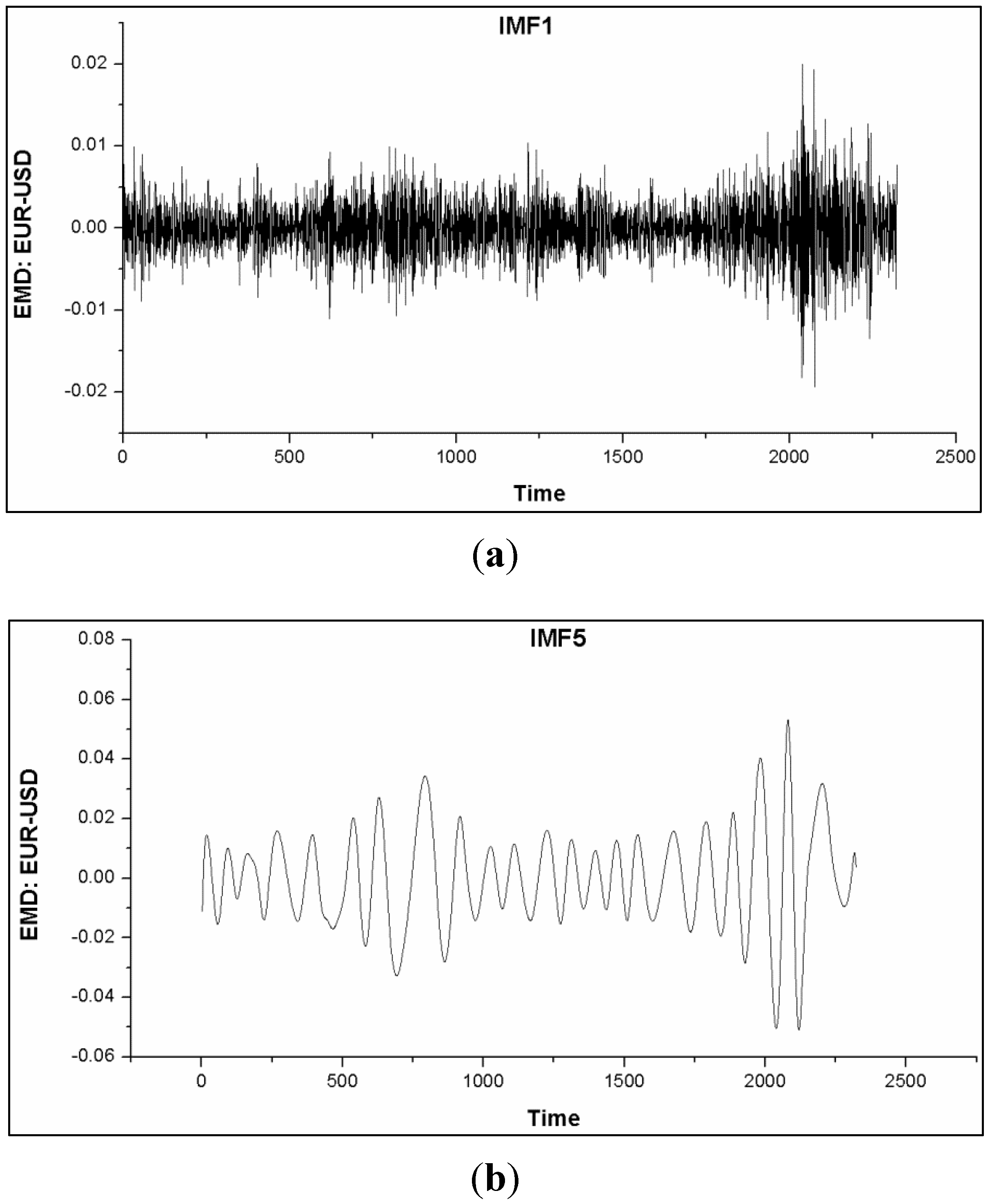
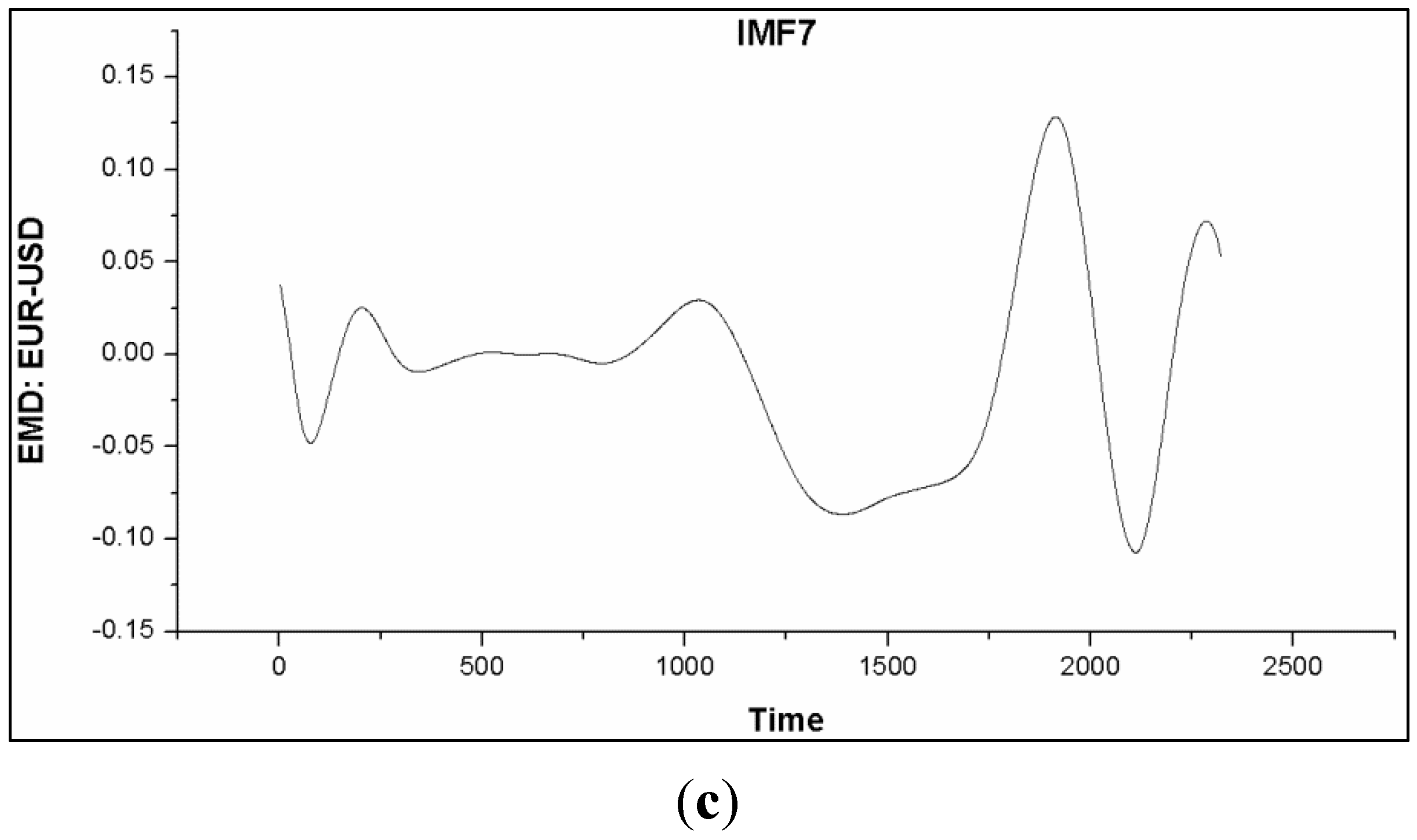
Based on the simulations of the algorithms namely; aIMF, WT, EKF and PF, we have found that the aIMF performed the best, following in the order to WT, EKF and PF. Theoretically, the successful application of EMD resides on the fact that the noise is not biased. Therefore, there is not so much of a restrictive constraint, comparing to the scenario of encountering with non-zero mean noise. As mentioned, the characteristics of IMF after several iterations move towards the normal distribution; see Figure 11. Thus, subtracting the averaged IMF with the original signals, given aIMF, can reduce the noise inevitably. However, the proposed aIMF algorithm using cubic spline interpolation does not intend to preserve edges of the datasets/signals. This is because of our target to reduce noise that may associate with the upper and lower boundaries of the curves, which are in time series domain. In this particular case, preserving the edges/curves can unavoidably keep the noise mixing within the signals. Unlike the images whose distribution is random walk, the noise reduction can be achieved while the edges are preserved [27]. Referring to Section 3.1, we manually added a variety of noises into the datasets with separate simulations; and later proved that the noises have been removed significantly, displayed in Figure 7 and Table 1, Table 2, Table 3, Table 4, Table 5 and Table 6. To continue to prove the aIMF algorithm’s performance, we simulated the aIMF algorithm with the original datasets—without adding extra noise. The results measured by MSE, MAE, MAPE, R² and Accuracy count were 8.20211E−05, 0.00719, 0.57085, 0.9980 and 99.95%, respectively. It is noted that the original datasets, EUR-USD exchange rates, contained a certain level of noise, not pure signal only. In the real application, data of exchange rates are normally fluctuated before closing hours of trading by retailers and speculators who want to manipulate the price. The manipulations are always executed with low volumes of trade, but enable the price changes at the end of trading hours. In the financial community, we deem these trades as noise. Finally, the figures from the last loss estimators shown were similar to the results in Table 1, Table 2, Table 3, Table 4, Table 5 and Table 6. Hence, it is safe to assume that the proposed aIMF algorithm can remove the unwanted signals.

Figure 11. Graphs (a)–(c) show plots of IMF1, IMF5 and IMF7, of which their local extrema of higher order IMF moved toward the normal distribution.

Figure 11. Graphs (a)–(c) show plots of IMF1, IMF5 and IMF7, of which their local extrema of higher order IMF moved toward the normal distribution.

On another front, the simulation results from the WT algorithm seemed to be unacceptable under the rationale that Fourier spectral analysis and its derivatives such as WT encountered with a limited time window width by sliding a predetermined window(s) along the time axis [28]. Moreover, there is a trade-off between the time consumed in the window width and the frequency resolution, and this phenomenon has been considered by the uncertainty principle Heisenberg [21]. In this particular case, the WT’s window width must be preselected and it is known as the primary or mother wavelet which is a prototype that provides less flexibility when handling datasets were the mean and variances are highly volatile. In case of EKF simulation, the advantage of SIS is that it does not guarantee to fail as time increases and it becomes more and more skewed, especially when sampling high-dimensional spaces [26]. For the PF algorithm, we have found that the number of particles (data-points) was not adequate for Monte Carlo simulation. However, the drawback of the aIMF algorithm is that it requires long time to spline the local extrema.

3.7. Robustness Test

Robustness testing is any quality assurance methodology focused on testing the consistent accuracy of software. In this section, we test the algorithms of aIMF, WT, EKF and PF which function as noise reduction models. The testing strategies used different inputs other than the EUR-USD exchange rates with the added noise, which are created from 1 Hz sine wave at 10% amplitude of the original datasets with the 10% random distribution. Those different inputs are EUR-JPY with the added noise, EUR-CHF with the added noise, finally, EUR-GBP with the added noise. Later, we used loss estimators to measure the prediction performances of the proposed aIMF, WT, EKF and PF, i.e., MSE, MAE, MAPE, R², AIC, BIC and Accuracy count. Having simulated with all the loss estimators indicated in Table 7, Table 8 and Table 9 under the same conditions used to test for EUR-USD as input, the results shared the same trend with few deviations from each other. This served to confirm that the aIMF algorithm performed significantly better when filtering a nonlinear nonstationary time series, i.e., EUR-JPY, EUR-CHF and EUR-GBP exchange rates, followed by WT and EKF algorithms. Moreover, we rejected using the PF algorithm to reduce the noise for the nonlinear nonstationary time series data. Additionally, we have discovered that the EKF and WT algorithm must be optimised in the areas of resampling and building up mother wavelet, respectively.

Table 7. Performance measurements of original dataset, EUR-JPY, using noise distribution at 10% with 10 Hz and 20% amplitude of the original signals’.

EUR-JPY	MSE	MAE	MAPE	R2	AIC	BIC	Accuracy count (%)
aIMF	0.00424	0.057854	8.29746	0.5219	−6782.23	−6764.98	63.85
WT	0.00626	0.05676	8.67169	0.5514	−6839.68	−682.42	53.46
EKF	0.00516	0.063797	9.15559	0.4046	−6272.94	−6255.69	49.50
PF	3.37133	1.42611	204.696	0.0020	−5074.33	−5057.08	50.19

Table 7. Performance measurements of original dataset, EUR-JPY, using noise distribution at 10% with 10 Hz and 20% amplitude of the original signals’.

EUR-JPY	MSE	MAE	MAPE	R2	AIC	BIC	Accuracy count (%)
aIMF	0.00424	0.057854	8.29746	0.5219	−6782.23	−6764.98	63.85
WT	0.00626	0.05676	8.67169	0.5514	−6839.68	−682.42	53.46
EKF	0.00516	0.063797	9.15559	0.4046	−6272.94	−6255.69	49.50
PF	3.37133	1.42611	204.696	0.0020	−5074.33	−5057.08	50.19

Table 8. Performance measurements of original dataset, EUR-CHF, using noise distribution at 10% with 10 Hz and 20% amplitude of the original signals’.

EUR-CHF	MSE	MAE	MAPE	R2	AIC	BIC	Accuracy count (%)
aIMF	0.03772	0.145457	0.420782	0.9983	−1086.41	−1069.16	88.96
WT	0.08124	0.1745481	0.53478	0.5905	−6852.24	−6699.54	53.20
EKF	0.37038	0.176222	0.519026	0.5588	−11843.6	−11860.9	45.71
PF	1218.50	34.52886	101.8893	0.4421	−12388.2	−12405.5	50.84

Table 8. Performance measurements of original dataset, EUR-CHF, using noise distribution at 10% with 10 Hz and 20% amplitude of the original signals’.

EUR-CHF	MSE	MAE	MAPE	R2	AIC	BIC	Accuracy count (%)
aIMF	0.03772	0.145457	0.420782	0.9983	−1086.41	−1069.16	88.96
WT	0.08124	0.1745481	0.53478	0.5905	−6852.24	−6699.54	53.20
EKF	0.37038	0.176222	0.519026	0.5588	−11843.6	−11860.9	45.71
PF	1218.50	34.52886	101.8893	0.4421	−12388.2	−12405.5	50.84

Table 9. Performance measurements of original dataset, EUR-GBP, using noise distribution at 10% with 10 Hz and 20% amplitude the original signals’.

EUR-CHF	MSE	MAE	MAPE	R2	AIC	BIC	Accuracy count (%)
aIMF	0.00424	0.057854	8.306478	0.5191	−6802.20	−6784.98	64.92
WT	0.00826	0.065946	9.319482	0.6435	−6699.65	−6382.98	51.08
EKF	0.00517	0.063851	9.171988	0.4055	−6309.97	−6292.68	49.20
PF	3.33789	1.435658	206.7395	0.0006	−5104.53	−5087.27	48.68

Table 9. Performance measurements of original dataset, EUR-GBP, using noise distribution at 10% with 10 Hz and 20% amplitude the original signals’.

EUR-CHF	MSE	MAE	MAPE	R2	AIC	BIC	Accuracy count (%)
aIMF	0.00424	0.057854	8.306478	0.5191	−6802.20	−6784.98	64.92
WT	0.00826	0.065946	9.319482	0.6435	−6699.65	−6382.98	51.08
EKF	0.00517	0.063851	9.171988	0.4055	−6309.97	−6292.68	49.20
PF	3.33789	1.435658	206.7395	0.0006	−5104.53	−5087.27	48.68

The following configurations were used to perform all the simulations:

(i)

Intel(R) Xeon(R) server with 2 × 2.4 GHz E5620 CPUs, 3.99 GB RAM and a 64-bit Microsoft Windows Operating System is configured as the main processor.

(ii)

Sony Visio, Sony L2412M1EB Desktop with an Intel Core i5, 2.5 GHz, 8 GB RAM, and a 64-bit Microsoft Windows Operating System is used as the front-end connection to the data terminal from Bloomberg via web access using a Citrix client.

(iii)

Application programs written using R programming scripts and some amendments to suit the requirements.

The simulation results showed that there were no bugs in the software scripts, and an average execution time of 3 s for all the Ordinary Least Square (OLS) models.

4. Conclusion

Noise reduction for a nonlinear nonstationary time series is challenging since the models require a large amount of computational power and more complicated logic than conventional filters. This paper proposed a new filter, the aIMF algorithm, which demonstrated its accuracy and robustness, compared with the WT, EKF and PF algorithms. In this study, we discovered that PF is not suitable for this kind of work. Additionally, the EKF and WT algorithms should be optimised. It may be because the number of particles for sampling and weights were not enough albeit the number of data-points used were more than 2000. Future work to enhance the efficiency of the aIMF algorithm are in the area of (i) optimising the cubic spline algorithm to be more suitable to the input which sometimes persisted to its mean, and (ii) investigating the possibility of designing a DSP chip for the aIMF algorithm.

References

1. Huttunen, J.M.J.; Lehikoinen, A.; Hämäläinen, J.; Kaipio, J. Importance sampling approach for the nonstationary approximation error method. Inverse Probl. 2002, 26, 1–16. [Google Scholar]
2. Brown, R.G.; Hwang, P.Y.C. Introduction to Random Signals and Applied Kalman Filtering, 3rd ed.; John Wiley & Sons, Inc.: New Jersey, NJ, USA, 1992; pp. 128–140. [Google Scholar]
3. Calabrese, A.; Paninski, L. Kalman filter mixture model for spike sorting of nonstationary data. J. Neurosci. Methods 2011, 196, 159–169. [Google Scholar] [CrossRef] [PubMed]
4. Sanjeev Arulampalam, M.; Maskell, S.; Gordon, N.; Clapp, T. A tutorial on particle filters for online nonlinear/non-gaussian bayesian tracking. IEEE Trans. Signal Process. 2002, 50, 174–187. [Google Scholar] [CrossRef]
5. Caron, F.; Davy, M.; Duflos, E.; Vanheeghe, P. Particle filtering for multi-sensor data fusion with switching observation models: Applications to land vehicle positioning. IEEE Trans. Signal Process. 2007, 55, 2703–2719. [Google Scholar] [CrossRef]
6. Gustafsson, F.; Gunnarsson, F.; Bergman, N.; Forssel, U. Particle filters for positioning, navigation and tracking. IEEE Trans. Signal Process. 2002, 50, 425–437. [Google Scholar] [CrossRef]
7. Thrun, S.; Burgard, B.; Fox, D. Probabilistic Robotics; MIT Press: Massachusetts, MA, USA, 2005; pp. 39–117. [Google Scholar]
8. Huang, N.E.; Attoh-Okine, N.O. The Hilbert Transform in Engineering; CRC Press, Taylor & Francis Group: Florida, FL, USA, 2005. [Google Scholar]
9. Wu, Z.; Huang, N.E. Ensemble empirical mode decomposition: A noise-assisted data analysis method. Adv. Adapt. Data Anal. 2009, 1, 1–41. [Google Scholar] [CrossRef]
10. Huang, W.; Shen, Z.; Huang, N.E.; Fung, Y.C. Nonlinear indicial response of complex nonstationary oscillations as pulmonary hypertension responding to step hypoxia. Proc. Natl. Acad. Sci. USA 1996, 96, 1834–1839. [Google Scholar] [CrossRef]
11. Huang, N.E.; Shen, Z.; Long, S.R. The empirical mode decomposition and the hilbert spectrum for nonlinear and nonstationary time series analysis. Proc. R. Soc. Lond. A 1998, 454, 903–995. [Google Scholar] [CrossRef]
12. Huang, N.E.; Shen, S.S.P. Hilbert-Huang Transform and Its Applications; World Scientific Publishing Company: Singapore, 2005; pp. 2–26. [Google Scholar]
13. Wang, L.; Koblinsky, C.; Howden, S.; Huang, N.E. Interannual variability in the South China Sea from expendable bathythermograph data. J. Geophys. Res. 1990, 104, 509–523. [Google Scholar] [CrossRef]
14. Datig, M.; Schlurmann, T. Performance and limitations of the Hilbert-Huang Transformation (HHT) with an application to irregular water waves. Ocean Eng. 2004, 31, 1783–1834. [Google Scholar] [CrossRef]
15. Guhathakurta, K.; Mukherjee, I.; Roy, A. Empirical mode decomposition analysis of two different financial time series and their comparison, Chaos. Solut. Fractals 2008, 37, 1214–1227. [Google Scholar] [CrossRef]
16. Cohen, L. Frequency analysis. IEEE Trans. Signal Process. 1995, 55, 2703–2719. [Google Scholar]
17. Kaslovsky, D.N.; Meyer, F.G. Noise corruption of empirical mode decomposition and its effect on instantaneous frequency. Adv. Adapt. Data Anal. 2010, 2, 373–396. [Google Scholar] [CrossRef]
18. Flandrin, P.; Rilling, G.; Goncalves, P. Empirical mode decomposition as a filter Bank. IEEE Signal Process. Lett. 2004, 11, 112–114. [Google Scholar] [CrossRef]
19. Peng, Z.K.; Tse, P.W.; Chu, F.L. An improved Hilbert-Huang transform and its application in vibration signal analysis. J. Sound Vib. 2005, 286, 187–205. [Google Scholar] [CrossRef]
20. Gilks, W.R.; Richardson, S.; Spiegelhalter, D.J. Morkov Chain Monte Carlo in Practice; Chapman & Hall/CRC: Florida, FL, USA, 1996; p. 1. [Google Scholar]
21. Heisenberg, W. Physical Principles of the Quantum Theory; The University of Chicago Press: Chicago, IL, USA, 1930. [Google Scholar]
22. Kaiser, G. A Friendly Guide to Wavelets; Birkhause: Boston, MA, USA, 1994; pp. 44–45. [Google Scholar]
23. Helong, L.; Xiaoyan, D.; Hongliang, D. Structural damage detection using the combination method of EMD and wavelet analysis. Mech. Syst. Signal Process. 2007, 21, 298–306. [Google Scholar]
24. Li, L. On the block thresholding wavelet estimators with censored data. J. Multivar. Anal. 2008, 9, 1518–1543. [Google Scholar] [CrossRef]
25. Stein, C. Estimation of the mean of a multivariate normal distribution. Annu. Stat. 1981, 9, 1135–1151. [Google Scholar] [CrossRef]
26. Dang, D.S.; Weifeng, T.; Feng, Q. EMD- and LWT-based stochastic noise eliminating method for fiber optic gyro. Measurement 2010, 44, 2190–2193. [Google Scholar] [CrossRef]
27. Palma, R.; Vmoraru, C.; Woo, J. Pahikkala, Parseval Equality, version 8; 2012. Available online: http://planetmath.org/?op=getobj;from=objects;id=4717 (accessed on 12 December 2012).
28. Randhawa, S.; Li, J.J.S. Adaptive Order Spline Interpolation for Edge-Preserving Colour Filter Array Demosaicking. In Proceeding of the 2011 International Conference on Digital Image Computing: Techniques and Applications (DICTA), Noosa, QLD, Australia, 6–8 December 2011; pp. 666–671. [CrossRef]