New Heuristics for Rooted Triplet Consistency ^†

Abstract

Rooted triplets are becoming one of the most important types of input for reconstructing rooted phylogenies. A rooted triplet is a phylogenetic tree on three leaves and shows the evolutionary relationship of the corresponding three species. In this paper, we investigate the problem of inferring the maximum consensus evolutionary tree from a set of rooted triplets. This problem is known to be APX-hard. We present two new heuristic algorithms. For a given set of m triplets on n species, the FastTree algorithm runs in $O(m+\alpha \left(n\right)n^2)$ time, where $\alpha \left(n\right)$ is the functional inverse of Ackermann’s function. This is faster than any other previously known algorithms, although the outcome is less satisfactory. The Best Pair Merge with Total Reconstruction (BPMTR) algorithm runs in $O\left(m{n}^3\right)$ time and, on average, performs better than any other previously known algorithms for this problem.

1. Introduction

After the publication of Charles Darwin’s book On the Origin of Species by Means of Natural Selection, the theory of evolution was widely accepted. Since then, remarkable developments in evolutionary studies brought scientists to phylogenetics, a field that studies the biological or morphological data of species to output a mathematical model, such as a tree or a network, representing the evolutionary interrelationship of species and the process of their evolution. Interestingly, phylogenetics is not only limited to biology, but may also arise anywhere that the concept of evolution appears. For example, a recent study in evolutionary linguistics employs a phylogeny inference to clarify the origin of the Indo-European language family [1]. Several approaches have been introduced to infer evolutionary relationships [2]. Among those, well-known approaches are character-based methods (e.g., maximum parsimony), distance-based methods (e.g., neighbor joining and UPGMA) and quartet-based methods (e.g., QNet). Recently, rather new approaches, namely, triplet-based methods, have been introduced. Triplet-based methods output rooted trees and networks, due to the rooted nature of triplets. A rooted triplet is a rooted unordered leaf-labeled binary tree on three leaves and shows the evolutionary relationship of the corresponding three species. Triplets can be obtained accurately using a maximum likelihood method, such as the one introduced by Chor et al. [3], or the Sibley-Ahlquist-style DNA-DNA hybridization experiments [4]. Indeed, we expect highly accurate results from triplet-based methods. However, sometimes, due to experimental errors or some biological events, such as hybridization (recombination) or horizontal gene transfer, it is not possible to reconstruct a tree that satisfies all of the input constraints (triplets). There are two ways to overcome this problem. The first approach is to employ a more complex model, such as a network, which is the proper approach when the mentioned biological events have actually happened. The second approach tries to reconstruct a tree satisfying as many input triplets as possible. This approach is more useful when the input data contains errors. The latter approach forms the subject of this paper. In the next section, we will provide necessary definitions and notations. Section 3 contains an overview of previous results. We will present our algorithms and experimental results in Section 4. Finally, in Section 5, open problems and ideas for further improvements are discussed.

2. Preliminaries

An evolutionary tree (phylogenetic tree) on a set, S, of n species, $\left|S\right|=n$, is a rooted binary (More precisely, an evolutionary tree can also be unrooted; however, triplet-based methods output rooted phylogenies)unordered tree in which leaves are distinctly labeled by members of S (see Figure 1a). A rooted triplet is a phylogenetic tree with three leaves. The unique triplet of leaves, x, y, z, is denoted by ((x, y), z) or xy|z, if the lowest common ancestor of x and y is a proper descendant of the lowest common ancestor of x and z or, equivalently, if the lowest common ancestor of x and y is a proper descendant of the lowest common ancestor of y and z (see Figure 1b). A triplet, t (e.g., xy|z) is consistent with a tree, T, or, equivalently, T is consistent with t) if t is an embedded subtree of T. This means that t can be obtained from T by a series of edge contractions (i.e., if in T, the lowest common ancestor of x and y is a proper descendant of the lowest common ancestor of x and z). We also say T satisfies t, if T is consistent with t. The tree in Figure 1a is consistent with the triplet in Figure 1b. A phylogenetic tree, T, is consistent with a set of rooted triplets if it is consistent with every triplet in the set. We call two leaves siblings or a cherry if they share the same parent. For example, {x, y} in Figure 1a form a cherry.

Figure 1. Example of a phylogenetic tree and a consistent triplet. (a) A phylogenetic tree; (b) the triplet xy|z.

A set of triplets, R, is called dense if for each set of three species, {x, y, z}, R, contains at least one of three possible triplets, xy|z, xz|y or yz|x. If R contains exactly one triplet for each set of three species, it is called minimally dense, and if it contains every possible triplet, it is called maximally dense. Now, we can define the problem of reconstructing an evolutionary tree from a set of rooted triplets. Suppose S is a finite set of species of cardinality, n, and R is a finite set of rooted triplets of cardinality, m, on S. The problem is to find an evolutionary tree leaf-labeled by members of S, which is consistent with the maximum number of rooted triplets in R. This problem is called the Maximum Rooted Triplets Consistency (MaxRTC) problem [5] or the Maximum Inferred Local Consensus Tree (MILCT) problem [6]. This problem is NP-hard (see Section 3), which means no polynomial-time algorithm can be found to solve the problem optimally unless P= NP. For this and similar problems, one might search for polynomial-time algorithms that produce approximate solutions. We call an algorithm an approximation algorithm if its solution is guaranteed to be within some factor of optimum solution. In contrast, heuristics may produce good solutions, but do not come with a guarantee on their quality of solution. An algorithm for a maximization problem is called an $\alpha -approximation$ algorithm, for some $\alpha >1$, if for any input, the output of the algorithm is at most α-times worse than the optimum solution. The factor, α, is called the approximation factor or approximation ratio.

3. Related Works

Aho et al. [7] investigated the problem of constructing a tree consistent with a set of rooted triplets for the first time. They designed a simple recursive algorithm, which runs in $O\left(mn\right)$ time and returns a tree consistent with all of the given triplets, if at least one tree exists. Otherwise, it returns null. Later, Henzinger et al. [8] improved Aho et al.’s algorithm to run in $min\{O(n+m{n}^{1/2}),O(m+n^{2}logn)\}$ time. The time complexity of this algorithm was further improved to $min\{O(n+mlo{g}^{2}n),O(m+n^{2}logn)\}$ by Jansson et al. [9] using more recent data structures introduced by Holm et al. [10]. MaxRTC is proven to be NP-hard [6,11,12]. Byrka et al. [13] reported that this proof is an L-reduction from an APX-hard problem, meaning that the problem is APX-hard, in general (non-dense case). Later, Van Iersel et al. [14] proved that MaxRTC is NP-hard, even if the input triplet set is dense.

Several heuristics and approximation algorithms have been presented for the so-called MaxRTC problem, each performing better in practice on different input triplet sets. Gasieniec et al. [15] proposed two algorithms by modifying Aho et al.’s algorithm. Their first algorithm, which is referred to as One-Leaf-Split [5] runs in $O\left(\right(m+n\left)logn\right)$ time, and the second one, which is referred to as Min-Cut-Split [5], runs in $min\{O(m{n}^2+n^{3}logn),O\left(n^4\right)\}$ time. The tree generated by the first algorithm is guaranteed to be consistent with at least one third of the input triplet set. This gives a lower bound for the problem. In another study, Wu [11] introduced a bottom-up heuristic approach called BPMF (Best Pair Merge First), which runs in $O\left(m{n}^3\right)$ time. In the same study, he proposed an exact exponential algorithm for the problem, which runs in $O\left((m+n^2)3^n\right)$ time and $O\left(2^n\right)$ space. According to the results of Wu [11], BPMF seems to perform well on average on randomly generated data. Later, Maemura et al. [16] presented a modified version of BPMF, called BPMR (Best Pair Merge with Reconstruction), which employs the same approach, but with a little bit different of a reconstruction routine. BPMR runs in $O\left(m{n}^3\right)$ time and, according to Maemura et al.’s experiments, outperforms BPMF. Byrka et al. [13] designed a modified version of BPMF to achieve an approximation ratio of three. They also investigated how MinRTI (Minimum Rooted Triplet Inconsistency) can be used to approximate MaxRTC and proved that MaxRTC admits a polynomial-time, $(3-\frac{2}{n-2})-$, approximation.

4. Algorithms and Experimental Results

In this Section, we present two new heuristic algorithms for the MaxRTC problem.

4.1. FastTree

The first heuristic algorithm has a bottom-up greedy approach, which is faster than the other previously known algorithms employing a simple data structure.

Let R(T) denote the set of all triplets consistent with a given tree, T. R(T) is called the reflective triplet set of T. It forms a minimally dense triplet set and represents T uniquely [17]. Now, we define the closeness of the pair, {i,j}. The closeness of the pair, {i,j}, $C_{i,j}$, is defined as the number of triplets of the form, ij|k, in a triplet set. Clearly, for any arbitrary tree, T, the closeness of a cherry species equals $n-2$, which is maximum in R(T). The reason is that every cherry species has a triplet with every other species. Now, suppose we contract every cherry species of the form, {i,j}, to their parents, $p_{ij}$, and then update R(T) as follows. For each contracted cherry species, {i,j}, we remove triplets of the form, ij|k, from R(T) and replace i and j with $p_{ij}$ within the remaining triplets. The updated set, $R^{\prime }\left(T^{\prime }\right)$, would be the reflective triplet set for the new tree, $T^{\prime }$. Observe that, for cherries of the form, $\{p_{ij},k\}$, in $T^{\prime }$, $C_{i,k}$ and $C_{j,k}$ would equal n-3 in R(T). Similarly, for cherries of the form, $\{p_{ij},p_{kl}\}$, in $T^{\prime }$, $C_{i,k}$, $C_{j,k}$, $C_{i,l}$ and $C_{j,l}$ would equal n-4 in R(T). This forms the main idea of the first heuristic algorithm. We first compute the closeness of pairs of species by visiting triplets. Furthermore, sorting the pairs according to their closeness gives us the reconstruction order of the tree. This routine outputs the unique tree, T, for any given reflective triplet set, R(T). Yet, we have to consider that the input triplet set is not always a reflective triplet set. Consequently, the reconstruction order produced by sorting may not be the right order. However, if the loss of triplets admits a uniform distribution, it will not affect the reconstruction order. An approximate solution for this problem is refining the closeness. This can be done by reducing the closeness of the pairs, {i,k} and {j,k}, for any visited triplet of the form, ij|k. Thus, if the pair, {i,j}, is actually cherries, then the probability of choosing the pairs, {i,k} or {j,k}, before choosing the pair, {i,j}, due to triplet loss, will be reduced. We call this algorithm FastTree. See Algorithm 1 for the whole algorithm.

Algorithm 1 FastTree

1: Initialize a forest, F, consisting of n one-node trees labeled by species. 2: for each triplet of the form ij|k do 3:  $C_{i,j}$: = $C_{i,j}$+1 4:  $C_{i,k}$: = $C_{i,k}$−1 5:  $C_{j,k}$: = $C_{j,k}$−1 6: end for 7: Create a list, L, of pairs of species. 8: Sort L according to the refined closeness of pairs with a linear-time sorting algorithm. 9: while |L|>0 do 10:  Remove the pair, {i,j}, with maximum, $C_{i,j}$. 11:  if i and j are not in the same tree then 12:   Add a new node and connect it to roots of trees containing i and j. 13:  end if 14: end while 15: if F has more than one tree then 16:  Merge trees in any order, until there would be only one tree. 17: end if 18: return the tree in F

Theorem 1. FastTree runs in $O(m+\alpha \left(n\right)n^2)$ time.

Proof. Initializing a forest in Step 1 takes $O\left(n\right)$ time. Steps 2–6 take $O\left(m\right)$ time. We know that the closeness is an integer value between 0 and $n-2$. Thus, we can employ a linear-time sorting algorithm [18]. There are $O\left(n^2\right)$ possible pairs; therefore, Step 8 takes $O\left(n^2\right)$ time. Similarly, the while loop in Step 9 takes $O\left(n^2\right)$ time. Each removal in Step 10 can be done in $O\left(1\right)$ time. By employing optimal data structures, which are used for disjoint-set unions [18], the amortized time complexity of Steps 11 and 12 will be $O\left(\alpha \right(n\left)\right)$, where $\alpha \left(n\right)$ is the inverse of the function, $f\left(x\right)=A(n,n)$, and A is the well-known fast-growing Ackermann function. Furthermore, Step 16 takes $O\left(n\alpha \right(n\left)\right)$ time. Hence, the running time of FastTree would be $O(m+\alpha \left(n\right)n^2)$. ☐

Since $A(4,4)=2^{2^{2^{65536}}}$, $\alpha \left(n\right)$ is less than four for any practical input size, n. In comparison to the fast version of Aho et al.’s algorithm, FastTree employs a simpler data structure and, in comparison to Aho et al.’s original algorithm, it has lower time complexity. Yet, the most important advantage of FastTree to Aho et al.’s algorithm is that it will not stick if there is not a consistent tree with the input triplets, and it will output a proper tree in such a way that the clusters are very similar to that of the real network. 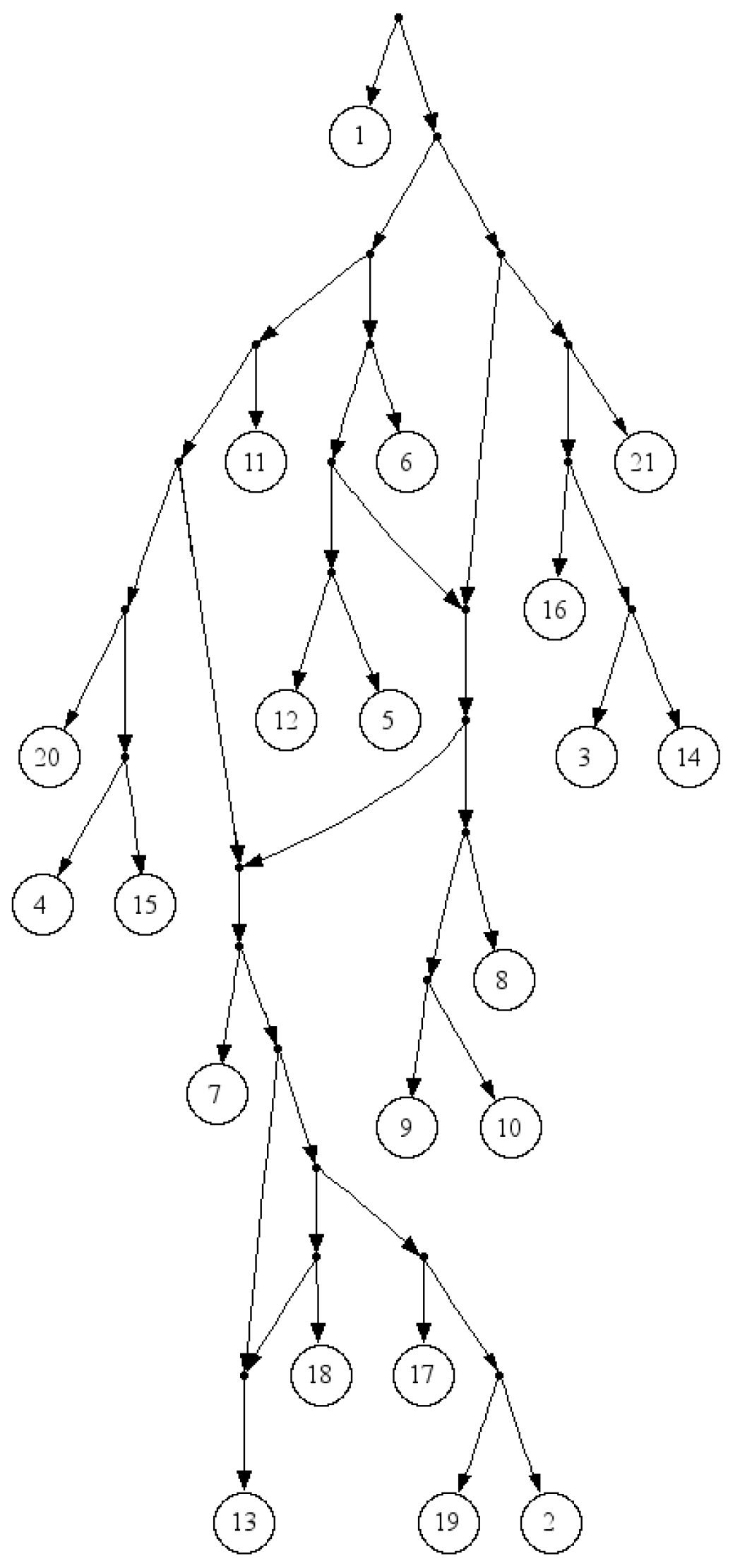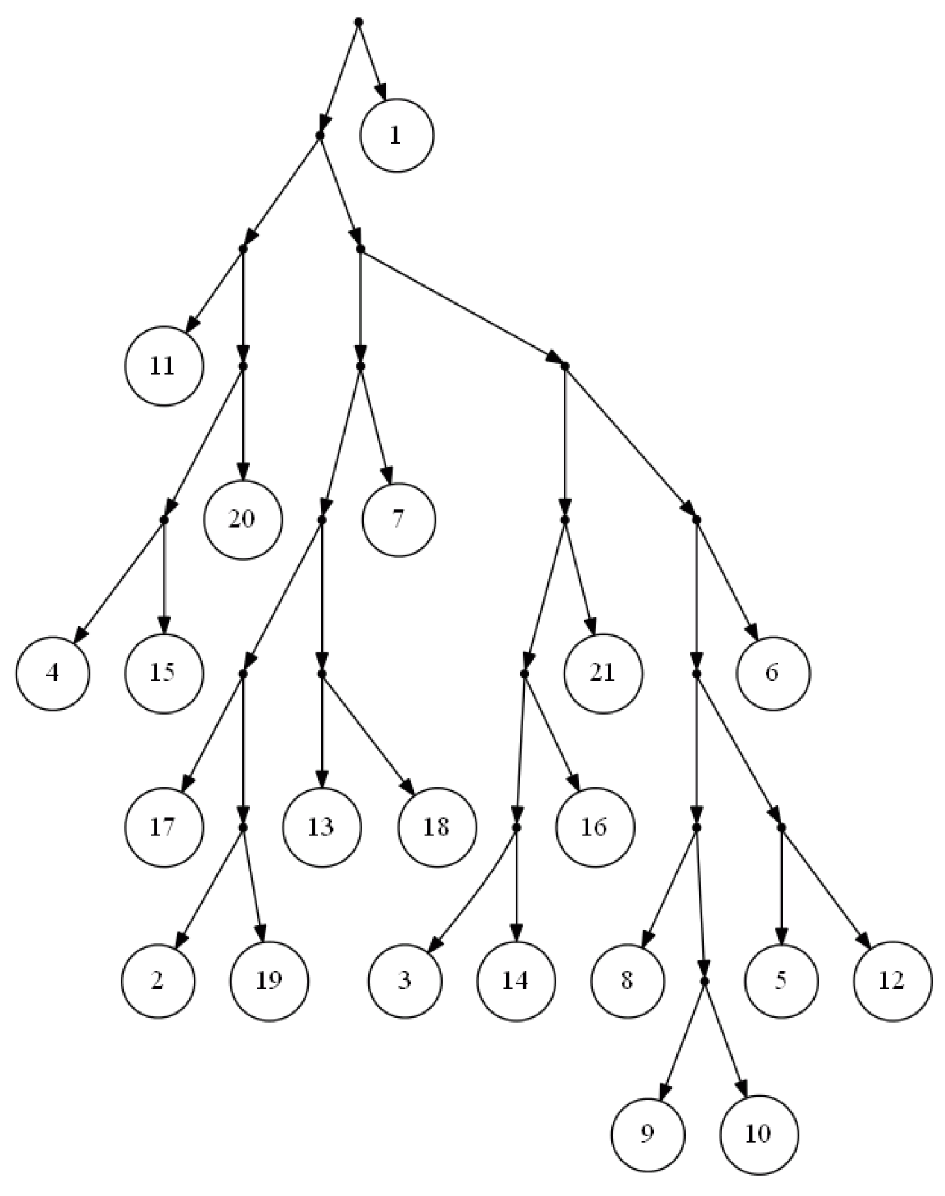The tree in Figure 2 is the output of FastTree on a dense set of triplets based on the yeast, Cryptococcus gattii, data. There is no consistent tree with the whole triplet set; however, Van Iersel et al. [19] presented a level-2 network consistent with the set (see Figure 3). This set is available online [20]. In comparison to BPMR and BPMF, FastTree runs much faster for large sets of triplets and species. However, for highly sparse triplet sets, the output of FastTree may satisfy considerably less triplets than the tree constructed by BPMF or BPMR.

Figure 2. Output of FastTree for a dense triplet set of the yeast, Cryptococcus gattii, data.

4.2. BPMTR

Before explaining the second heuristic algorithm, we need to review BPMF [11] and BPMR [16]. BPMF utilizes a bottom-up approach similar to hierarchical clustering. Initially, there are n trees, each containing a single node representing one of n given species. In each iteration, the algorithm computes a function, called $e\_score$, for each combination of two trees. Furthermore, two trees with the maximum $e\_score$ are merged into a single tree by adding a new node as the common parent of the selected trees. Wu [11] introduced six alternatives for computing the $e\_score$ using combinations of w, p and t. (see Table 1). However, in each run, one of the six alternatives must be used. In the function, $e\_score(C_1,C_2)$, w is the number of triplets satisfied by merging $C_1$ and $C_2$, which is the number of triplets of the form ij|k, in which i is in $C_1$, j is in $C_2$ and k is neither in $C_1$ nor in $C_2$. The value of p is the number of triplets that are in conflict with merging $C_1$ and $C_2$. It is the number of triplets of the form, ij|k, in which i is in $C_1$, k is in $C_2$ and j is neither in $C_1$ nor in $C_2$. The value of t is the total number of triplets of the form, ij|k, in which i is in $C_1$ and j is $C_2$. Wu compared the BPMF with One-Leaf-Split and Min-Cut-Split and showed that BPMF works better on randomly generated triplet sets. He also pointed out that none of the six alternatives of $e\_score$ is significantly better than the other.

Figure 3. A Level-2 network for a dense triplet set of the yeast, Cryptococcus gattii, data.

Table 1. The six alternatives of e_score.

If-Penalty		Ratio Type
False	w	w/(w + p)	w/t
True	w − p	(w − p)/(w + p)	(w − p)/t

Table 1. The six alternatives of e_score.

If-Penalty		Ratio Type
False	w	w/(w + p)	w/t
True	w − p	(w − p)/(w + p)	(w − p)/t

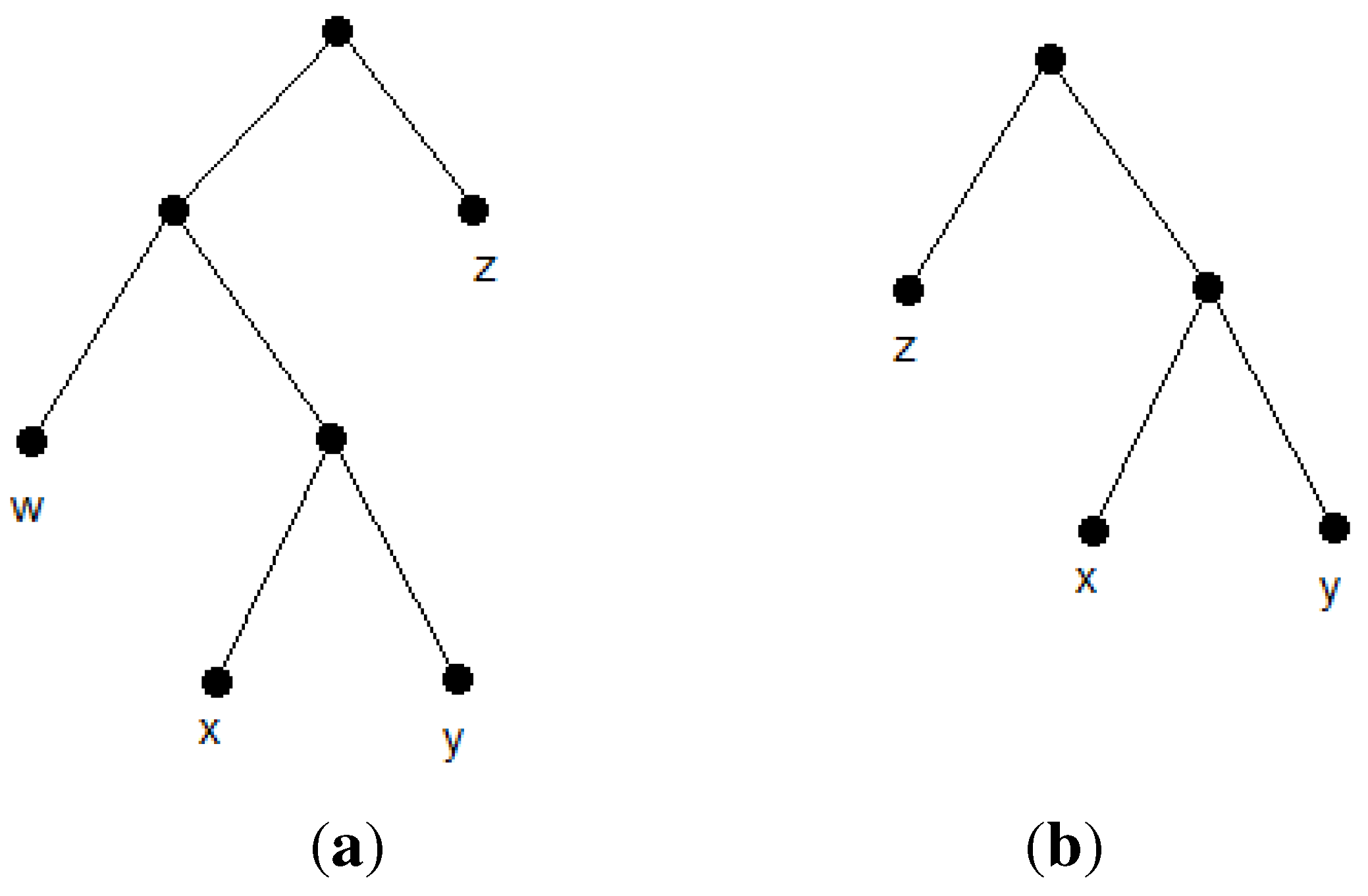
Maemura et al. [16] introduced a modified version of BPMF, called BPMR, that outperforms the results of BPMF. BPMR works very similarly in comparison to BPMF, except for a reconstruction step used in BPMR. Suppose $T_x$ and $T_y$ are two trees having the maximum, $e\_score$, at some iteration and are selected to merge into a new tree. By merging $T_x$ and $T_y$, some triplets will be satisfied, but some other triplets will be in conflict. Without loss of generality, suppose $T_x$ has two subtrees, namely the left subtree and the right subtree. In addition, suppose a triplet, ij|k, in which i is in the left subtree of $T_x$, k is in the right subtree of $T_x$ and j is in $T_y$. Observe that by merging $T_x$ and $T_y$, the mentioned triplet becomes inconsistent. However, swapping $T_y$ with the right subtree of the $T_x$ satisfies this triplet, while some other triplets become inconsistent. It is possible that the resulting tree of this swap satisfies more triplets than the primary tree. This is the main idea behind the BPMR. In BPMR, in addition to the regular merging of $T_x$ and $T_y$, $T_y$ is swapped with the left and the right subtree of $T_x$, and also, $T_x$ is swapped with the left and the right tree of $T_y$. Finally, among these five topologies, we choose the one that satisfies the most triplets.

Suppose the left subtree of the $T_x$ also has two subtrees. Swapping $T_y$ with one of these subtrees would probably satisfy new triplets, while some old ones would become inconsistent. There are examples in which this swap results in a tree that satisfies more triplets. This forms our second heuristic idea that swapping of $T_y$ with every subtree of $T_x$ should be checked. $T_x$ should also be swapped with every subtree of $T_y$. At every iteration of BPMF after choosing two trees maximizing the , the algorithm tests every possible swapping of these two trees with subtrees of each other and, then, chooses the tree with the maximum consistency of the triplets. We call this algorithm BPMTR (Best Pair Merge with Total Reconstruction). See Algorithm 2 for details of the BPMTR.

Algorithm 2 BPMTR

1: Initialize a set, T, consisting of n one-node trees labeled by species. 2: while |T|>1 do 3:  Find and remove two trees, $T_x$, $T_y$, with maximum $e\_score$. 4:  Create a new tree, $T_{merge}$, by adding a common parent to $T_x$ and $T_y$ 5:  $T_{best}$ : = $T_{merge}$ 6:  for each subtree $T_{sub}$ of $T_x$ do 7:   Let $T_{swapped}$ be the tree constructed by swapping $T_{sub}$ with $T_y$ 8:   if the number of consistent triplets with $T_{swapped}$ was larger than the number of triplets consistent with $T_{best}$ then 9:   $T_{best}$ : = $T_{swapped}$ 10:   end if 11:  end for 12:  for each subtree $T_{sub}$ of $T_y$ do 13:   Let $T_{swapped}$ be the tree constructed by swapping $T_{sub}$ with $T_x$ 14:   if the number of consistent triplets with $T_{swapped}$ was larger than the number of triplets consistent with $T_{best}$ then 15:    $T_{best}$ : = $T_{swapped}$ 16:   end if 17:  end for 18:  Add $T_{best}$ to T. 19: end while 20: return the tree in T

Theorem 2. BPMTR runs in $O\left(m{n}^3\right)$ time.

Proof. Step 1 takes $O\left(n\right)$ time. In Step 2, initially, T contains n clusters, but in each iteration, two clusters merge into a cluster. Hence, the while loop in Step 2 takes $O\left(n\right)$ time. In Step 3, $e\_score$ is computed for every subset of T of size two. By applying Bender and Farach-Colton’s preprocessing algorithm [21], which runs in $O\left(n\right)$ time for a tree with n nodes, every LCAquery can be answered in $O\left(1\right)$ time. Therefore, the consistency of a triplet with a cluster can be checked in $O\left(1\right)$ time. Since there are m triplets, Step 3 takes $\left(\genfrac{}{}{0pt}{}{\left|T\right|}{2}\right)O\left(m\right)$ time. In Steps 5, 9 and 15, $T_{best}$ is a pointer that stores the best topology found so far during each iteration of the while loop in $O\left(1\right)$ time. The complexity analysis of the loops in Steps 6–11 and 12–17 are similar, and it is enough to consider one. Every rooted binary tree with n leaves has $O\left(n\right)$ internal nodes, so the total number of swaps in Step 7 for any two clusters will be at most $O(n-|T\left|\right)$. In Step 8, computing the number of consistent triplets with $T_{swapped}$ takes no more than $O\left(m\right)$ time. Steps 4, 7 and 18 are implementable in $O\left(1\right)$ time. Accordingly, the running time of Steps 2–19 would be:

$${\displaystyle \sum _{\left|T\right|=2}^n\left[m\left(\genfrac{}{}{0pt}{}{\left|T\right|}{2}\right)+O(n-|T\left|\right)+m)\right]=O\left(m{n}^3\right)}$$

(1)

Step 20 takes $O\left(1\right)$ time. Hence, the time complexity of BPMTR is $O\left(m{n}^3\right)$. ☐

We tested BPMTR over randomly generated triplet sets with n = 15, 20 species and m = 500, 1,000 triplets. We experimented hundreds of times for each combination of n and m. The results in Table 2 indicate that BPMTR outperforms BPMR. However, in these hundreds of tests, there were a few examples of BPMR performing better than BPMTR. For n = 30 and m = 1,000, in 62 triplet sets out of a hundred randomly generated triplet sets, BPMTR satisfied more triplets. In 34 triplet sets, BPMR and BPMTR had the same results, and in four triplet sets, BPMR satisfied more triplets.

Table 2. Performance results of Best Pair Merge with Total Reconstruction (BPMTR) in comparison to Best Pair Merge with Reconstruction (BPMR).

No. of species and triplets	% better results	% worse results
n = 20, m = 500	%29	%0.0
n = 20, m = 1000	%37	%1
n = 30, m = 500	%61	%3
n = 30, m = 1000	%62	%4

Table 2. Performance results of Best Pair Merge with Total Reconstruction (BPMTR) in comparison to Best Pair Merge with Reconstruction (BPMR).

No. of species and triplets	% better results	% worse results
n = 20, m = 500	%29	%0.0
n = 20, m = 1000	%37	%1
n = 30, m = 500	%61	%3
n = 30, m = 1000	%62	%4

5. Conclusion and Unsolved Problems

In this paper, we presented two new algorithms for the so-called MaxRTC problem. For a given set of m triplets on n species, the FastTree algorithm runs in $O(m+\alpha \left(n\right)n^2)$ time, which is faster than any other previously known algorithm, although the outcome can be less satisfactory for highly sparse triplet sets. The BPMTR algorithm runs in $O\left(m{n}^3\right)$ time and, on average, performs better than any other previously known approximation algorithm for this problem. There is nonetheless still more room for improvement of the described algorithms.

1. In the FastTree algorithm, in order to compute the closeness of pairs of species, we check triplets, and for each triplet of the form, ij|k, we add a weight, w, to $C_{i,j}$ and subtract a penalty, p, from $C_{i,k}$ and $C_{j,k}$. In this paper, we set $w=p=1$. If one assigns different values for w and p, the closeness of the pairs of species will be changed, and the reconstruction order will be affected. It would be interesting to check for which values of w and p FastTree performs better.

2. Wu [11] introduced six alternatives for $e\_score$, each of which performs better for different input triplet sets. It would be interesting to find a new function that can outperform all the alternatives for any input triplet set.

3. The best-known approximation factor for the MaxRTC problem is three [13]. This is the approximation ratio of BPMF. Since MaxRTC is APX-hard, a PTASis unattainable, unless P = NP. However, [5] suggests that an approximation ratio in the region of 1.2 might be possible. Finding an $\alpha -$approximation algorithm for MaxRTC with $\alpha <3$ is still open.

4. It would also be interesting to find the approximation ratio of FastTree, in general, and for reflective triplet sets.

References

- Bouckaert, R.; Lemey, P.; Dunn, M.; Greenhill, S.J.; Alekseyenko, A.V.; Drummond, A.J.; Gray, R.D.; Suchard, M.A.; Atkinson, Q.D. Mapping the origins and expansion of the Indo-European language family. Science 2012, 337, 957–960. [Google Scholar] [CrossRef] [PubMed]
- Felsenstein, J. Inferring Phylogenies; Sinauer Associates: Sunderland, MA, USA, 2004. [Google Scholar]
- Chor, B.; Hendy, M.; Penny, D. Analytic Solutions for Three-Taxon MLMC Trees with Variable Rates Across Sites. In Algorithms in Bioinformatics; Gascuel, O., Moret, B., Eds.; Springer: Berlin, Germany, 2001; Lecture Notes in Computer Science, Volume 2149, pp. 204–213. [Google Scholar]
- Kannan, S.K.; Lawler, E.L.; Warnow, T.J. Determining the evolutionary tree using experiments. J. Algorithms 1996, 21, 26–50. [Google Scholar] [CrossRef]
- Byrka, J.; Gawrychowski, P.; Huber, K.T.; Kelk, S. Worst-case optimal approximation algorithms for maximizing triplet consistency within phylogenetic networks. J. Discret. Algorithms 2010, 8, 65–75. [Google Scholar] [CrossRef]
- Jansson, J. On the complexity of inferring rooted evolutionary trees. Electron. Notes Discret. Math. 2001, 7, 50–53. [Google Scholar] [CrossRef]
- Aho, A.V.; Sagiv, Y.; Szymanski, T.G.; Ullman, J.D. Inferring a tree from lowest common ancestors with an application to the optimization of relational expressions. SIAM J. Comput. 1981, 10, 405–421. [Google Scholar] [CrossRef]
- Henzinger, M.R.; King, V.; Warnow, T. Constructing a tree from homeomorphic subtrees, with applications to computational evolutionary biology. Algorithmica 1999, 24, 1–13. [Google Scholar] [CrossRef]
- Jansson, J.; Ng, J.H.K.; Sadakane, K.; Sung, W.K. Rooted Maximum Agreement Supertrees. Algorithmica 2005, 43, 293–307. [Google Scholar] [CrossRef]
- Holm, J.; de Lichtenberg, K.; Thorup, M. Poly-logarithmic deterministic fully-dynamic algorithms for connectivity, minimum spanning tree, 2-edge, and biconnectivity. J. ACM 2001, 48, 723–760. [Google Scholar] [CrossRef]
- Wu, B.Y. Constructing the maximum consensus tree from rooted triples. J. Comb. Optim. 2004, 8, 29–39. [Google Scholar]
- Bryant, D. Building Trees, Hunting for Trees, and Comparing Trees—Theory and Methods in Phylogenetic Analysis. PhD thesis, University of Canterbury, 1997. [Google Scholar]
- Byrka, J.; Guillemot, S.; Jansson, J. New Results on Optimizing Rooted Triplets Consistency. In Algorithms and Computation; Hong, S.H., Nagamochi, H., Fukunaga, T., Eds.; Springer: Berlin, Germany, 2008; Lecture Notes in Computer Science, Volume 5369, pp. 484–495. [Google Scholar]
- Van Iersel, L.; Kelk, S.; Mnich, M. Uniqueness, intractability and exact algorithms: Reflections on level-k phylogenetic networks. J. Bioinform. Comput. Biol. 2009, 7, 597–623. [Google Scholar] [PubMed]
- Gasieniec, L.; Jansson, J.; Lingas, A.; Ostlin, A. On the complexity of constructing evolutionary trees. J. Comb. Optim. 1999, 3, 183–197. [Google Scholar] [CrossRef]
- Maemura, K.; Jansson, J.; Ono, H.; Sadakane, K.; Yamashita, M. Approximation Algorithms for Constructing Evolutionary Trees from Rooted Triplets. In Proceedings of 10th Korea-Japan Joint Workshop on Algorithms and Computation, Gwangju, Korea, 9–10 August 2007.
- Jansson, J.; Sung, W.K. Inferring a level-1 phylogenetic network from a dense set of rooted triplets. Theor. Comput. Sci. 2006, 363, 60–68. [Google Scholar] [CrossRef]
- Cormen, T.T.; Leiserson, C.E.; Rivest, R.L. Introduction to Algorithms; MIT Press: Cambridge, MA, USA, 1990. [Google Scholar]
- Van Iersel, L.; Keijsper, J.; Kelk, S.; Stougie, L.; Hagen, F.; Boekhout, T. Constructing Level-2 Phylogenetic Networks from Triplets. In Research in Computational Molecular Biology; Vingron, M., Wong, L., Eds.; Springer: Berlin, Germany, 2008; Lecture Notes in Computer Science, Volume 4955, pp. 450–462. [Google Scholar]
- Kelk, S. LEVEL2: A fast algorithm for constructing level-2 phylogenetic networks from dense sets of rooted triplets. 2008. [Google Scholar]
- Bender, M.A.; Farach-Colton, M. The LCA Problem Revisited. In LATIN 2000: Theoretical Informatics; Gonnet, G., Viola, A., Eds.; Springer: Berlin, Germany, 2000; Lecture Notes in Computer Science, Volume 1776, pp. 88–94. [Google Scholar]
© 2013 by the authors; licensee MDPI, Basel, Switzerland. This article is an open access article distributed under the terms and conditions of the Creative Commons Attribution license (http://creativecommons.org/licenses/by/3.0/).