Article

Compression-Based Tools for Navigation with an Image Database

by
Antonella Di Lillo
1,
Ajay Daptardar
1,
Kevin Thomas
1,
James A. Storer
1,* and
Giovanni Motta
2
1
Computer Science Department, Brandeis University, Waltham, MA 02454, USA
2
Google Incorporated, 1600 Amphitheatre Parkway Mountain View, CA 94043, USA
*
Author to whom correspondence should be addressed.
Algorithms 2012, 5(1), 1-17; https://doi.org/10.3390/a5010001
Submission received: 23 August 2011 / Revised: 6 December 2011 / Accepted: 19 December 2011 / Published: 10 January 2012
(This article belongs to the Special Issue Data Compression, Communication and Processing)

Abstract

:
We present tools that can be used within a larger system referred to as a passive assistant. The system receives information from a mobile device, as well as information from an image database such as Google Street View, and employs image processing to provide useful information about a local urban environment to a user who is visually impaired. The first stage acquires and computes accurate location information, the second stage performs texture and color analysis of a scene, and the third stage provides specific object recognition and navigation information. These second and third stages rely on compression-based tools (dimensionality reduction, vector quantization, and coding) that are enhanced by knowledge of (approximate) location of objects.

1. Introduction

A typical scenario of interest consists of a user, who is visually impaired, walking along a city street and attempting to navigate a store entrance or intersection, with an interest in the identification and exact location of dynamic obstacles that may be stationary or moving (e.g., people) and static goals (e.g., traffic light button). We assume the user is equipped with a mobile device including a camera and access to an image database of the area such as Google Street View. The first stage of our proposed system, called a passive assistant, approximately locates the subject via GPS (or most recent GPS data) and then employs image processing calculations with respect to the image database for determining an accurate location (computationally intensive steps can be performed with internet access to a server). The second stage employs texture and color analysis to segment and classify portions of the current scene. The third stage utilizes specific object recognition algorithms to provide dynamic information regarding obstacles such as people blocking a doorway, and static information such as the precise location of a traffic light button and information on signs. These tools also have applications to autonomous navigation.

2. Color Analysis

In past work, we have developed a color-based retrieval system based on a form of differential compression where similarity is measured by employing vector quantization (VQ) to compress one image in terms of a codebook based on a second image; that is, similar images tend to compress well with respect to the other as compared to less similar ones (Daptardar and Storer [1]). This kind of approach has been successful in the past for testing similarity of text (e.g., Shapira and Storer [2,3]), although it is a much different problem for imagery. We have implemented and experimented with a system that can be described at a high level as follows:
  • Preprocess the database by sub-sampling each image in the database to create a thumbnail, and by constructing a small VQ codebook for feature vectors derived from each thumbnail.
  • Given a query image, compress it with each codebook in the database and rank the images of the database in order of the achieved distortion (using mean squared error).
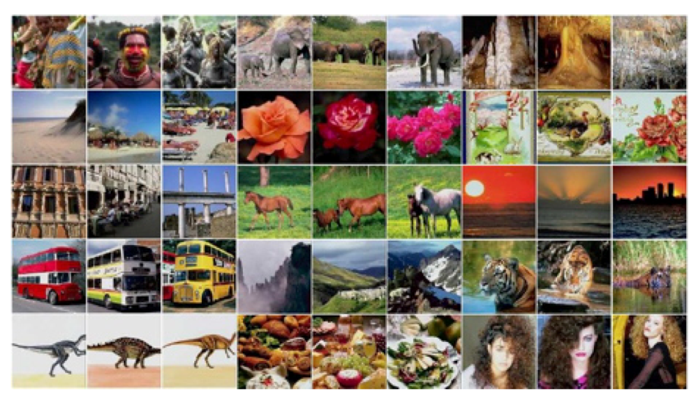
Preprocessing can be thought of as a tagging of images as they are added to the database. In fact, instead of the original images, the database may include only the codebook we construct and a link to the original image. For the query step, we have used forward compression, where database codebooks are used to compress the query image (rather than backward compression, where each image in the database is compressed with the codebook of the query image). We have chosen forward compression due both to its better performance and its extensive use in the previous work to which we have compared ours (e.g., Jeong and Gray [4]). In addition, as we address later in this paper, our specific design of forward compression can be implemented to run fast. To test our method, we have used as our database a subset of the COREL collection consisting of 1500 JPEG images, 100 in each of 15 classes (buses, horses, mountain scenes, etc.), an example of which is shown in Figure 1. The images in this database are already relatively small, but are still larger than is needed for a thumbnail. To create the database thumbnails, the system retains the central region (256 by 256 for these images) and scales it to 128 by 128 for each image (although it is possible to use smaller thumbnails, this size allows us to make direct comparisons with previous work). With our current system, the thumbnails are first transformed from the RGB color space to the perceptually uniform CIE LUV color space where the Euclidean distance between colors closely approximates their perceptual distance (Wyszecki and Stiles [5]). Feature vectors of 6 components each are then formed from the mean and variance of each color channel for each 2 × 2 block of a thumbnail. Once the feature vectors have been extracted, the VQ codebook for a thumbnail is constructed using a standard splitting algorithm (Gersho and Gray [6]) with MSE as the distance function.
Figure 1. Three sample images from each of the 15 classes in the COREL collection.
Algorithms 05 00001 g001
Retrieval effectiveness of a query is evaluated using standard precision vs. recall plots, where:
  • a = Number of relevant images (same class as the query) retrieved.
  • b = The number of irrelevant items that are retrieved
  • c = The number of relevant items that were not retrieved.
  • precision = fraction of the images retrieved that are relevant = a/(a + b)
  • recall = fraction of the relevant images that are retrieved = a/(a + c)
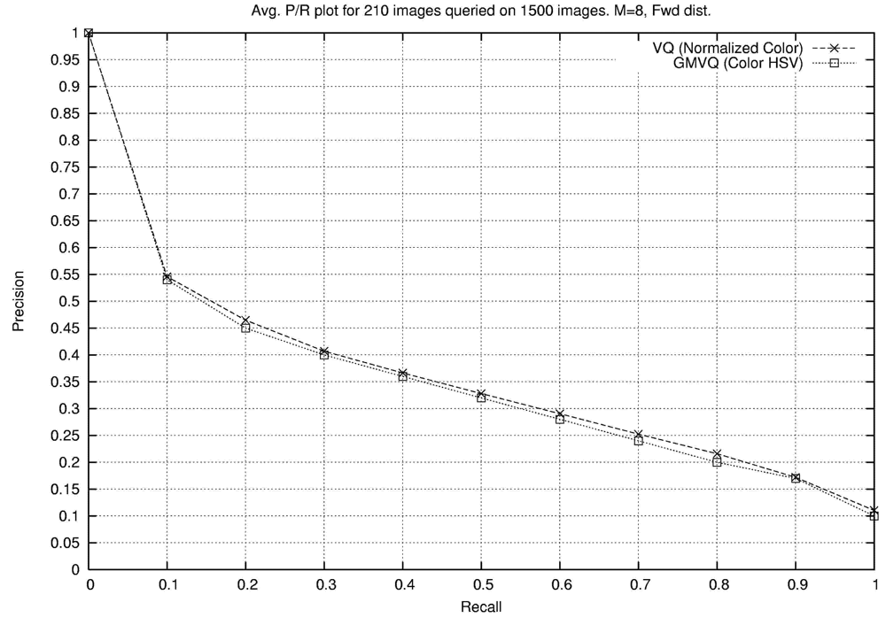
Precision and recall are shown on a single graph so that one may perceive the change in precision as the recall increases. Since the precision typically drops as the recall increases, a retrieval system is more effective when it has higher precision at the same recall level. Figure 2 compares our work with the GMVQ based system of Jeong and Gray [4]. In this work, the authors use image features that are in the HSV color space, which are obtained by a 4:1:1 sampling of the 2 × 2 HSV blocks (4 hue components together with one saturation and one value component). VQ codebooks of size 8 were computed for all images in the database.
Figure 2 indicates the average precision vs. recall when 210 images were queried. These images are the same ones that were chosen at random and used in the experiments reported by Jeong and Gray (results for our methods do not differ significantly for experiments where all 1500 images are queried—the 210 are used here simply to be consistent with Jeong and Gray [4]). Using the same code, with appropriate modifications (distance function, etc.), VQ retrieval used on average 1/3 of the time of GMVQ (that is, the total time to perform a retrieval of each of the 1500 images on the entire 1500 image set was more than three times greater for GMVQ). It can be seen from Figure 2 that although our VQ offers a lower complexity retrieval solution than GMVQ, the precision is not affected (in fact, it performs marginally better than GMVQ).
Figure 2. Our VQ (LUV Color) vs. GMVQ (HSV Color).
Algorithms 05 00001 g002

2.1. Explicit Incorporation of Position Information

Inherent to our system, as well as to the work of others such as the system of Jeong, Won, and Gray [7] or Wang [8], is a behavior that often functions as a bit of a two-edged sword. It is typical after a query to be surprised by images that strongly deviate from expectations. This is because, in some sense, quantization techniques are a generalization of color histogram measurement, which is subject to coincidences where two images that look obviously very different to a human just happen to have similar color distributions. For example, the four sets of images in Figure 3 show the top 12 images from four queries made to our current prototype system on the 1500 image COREL set (the upper left image of each set is the query image). As can be seen in Figure 3, the beach query has a number of responses from the mountains, one of the responses to the horse query comes from the elephant set, and one response from the elephant set comes from the beach set. In some cases, the top 12 responses are all from the correct class, as is the case for the architecture query. However, a basic limitation is that codebook entries are relatively small in dimension (e.g., feature vectors derived from 2 × 2 or 4 × 4 sub arrays of pixels) as compared to the image size, and do not capture global image structure.
To incorporate positional information, we have performed experiments with a straightforward approach where the mean XY coordinates of all blocks associated with a particular codebook entry are added to that entry (so the dimension of codebook entries is increased from 6 to 8). Figure 4 shows some database images with the code vector positions marked on the image. The color within each black-bordered box represents the color of the code vector. In order to appropriately weigh each feature (color and position), the two features (the 6-dimensional color feature and the 2-dimensional positional feature) are normalized. The distance between two feature vectors is computed using a weighted norm d(x, y) = (xy)tW(xy) where W is a diagonal weight matrix. The weight matrix was chosen empirically after performing tests on various weighing matrices that assigned different weights to the positional features.
Figure 3. Sample results.
Algorithms 05 00001 g003
Figure 4. Locations of code vectors within an image.
Algorithms 05 00001 g004
Figure 5. VQ with color only vs. VQ with color and position.
Algorithms 05 00001 g005
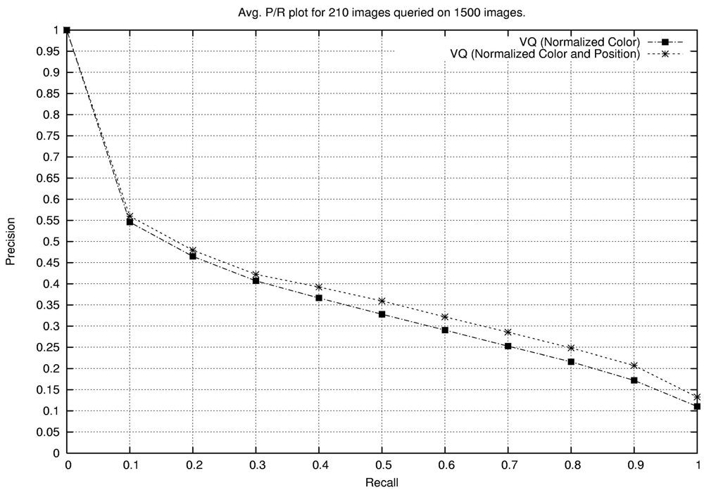
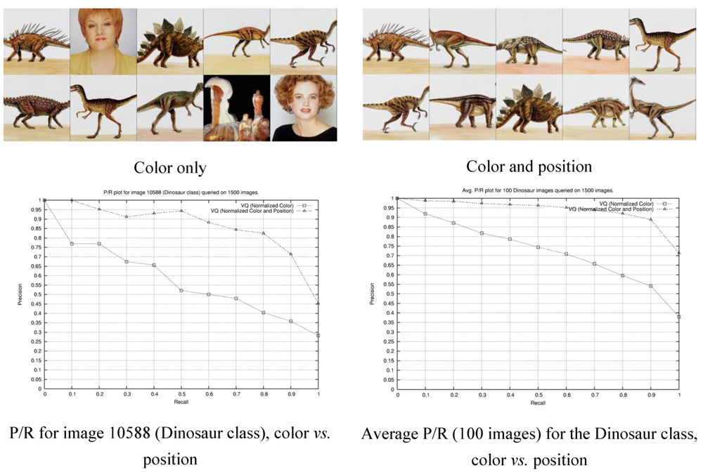
Using the same database and the same set of 210 query images as the previous section, Figure 5 compares our basic method using color only (6 element feature vectors) and color + XY (8 element feature vectors), again using codebooks of size 8. From this graph it can be seen that the use of extended feature vectors gives an overall modest improvement in performance. However, the real benefit of adding XY to the feature vector appears in classes with highly contrasting regions. For example, Figure 6 shows on the left the first 10 images retrieved for one of the dinosaur images with color only and on the right shows the first 10 for color + XY. For this query, the difference is highly significant, as can be seen from the graph on the left in Figure 6; the right shows the average of querying all 100 images in the dinosaur class, where again the difference can be seen as highly significant. In general, this straightforward addition of XY to the feature vectors provides “insurance”, where it makes little difference for many classes but can yield significant improvements for some. A drawback, however, is the need to choose the relative weighting empirically; we address this issue in the next section.
Figure 6. Color vs. color and position.
Algorithms 05 00001 g006

2.2. Region Based Retrieval

The simple approach of adding XY to feature vectors is encouraging. However, the introduction of XY into the VQ training is somewhat ad-hoc, and does introduce some added complexity (although still less complexity than the GMVQ approach to which we have made comparisons). We have performed a second set of experiments to implicitly incorporate positional information. The system computes similarity between corresponding image regions, where separate VQ codebooks trained on color feature vectors are associated with each region. To compare a query image with a database image, the total similarity score is the sum of the scores for each region, where the score for a region is the MSE when the query image features for that region are encoded using a database VQ codebook for that region. The size of each region’s codebook is varied by query and region by setting the query threshold. This parameter will determine how many codewords to use when encoding a query. Since the database codebook size needs to be varied based on the query image statistics, we use tree-structured codebooks (TSVQ) for the database images. After partitioning the image into regions, we train relatively large TSVQ codebooks by successively splitting nodes with the largest distortion until we arrive at the desired number of leaf codewords. That is, before codebooks of a given database image are used to encode the regions of the query image (to test similarity with that database image), each codebook is pruned to the same size as the codebook for that region associated with the query image. Figure 7 shows two images from the database and the number of codebook entries for each region using a threshold of 1500.
Figure 7. Sample region codebook sizes.
Algorithms 05 00001 g007
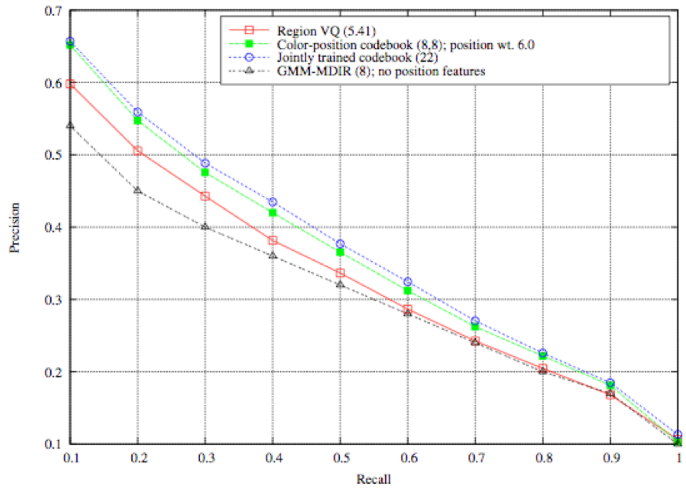
Figure 8. Region VQ compared to previous methods.
Algorithms 05 00001 g008
Experiments with threshold value have shown that best performance is achieved when average codebook size is 5.41 (Figure 8), but nearly identical (within 3%) and still better performance to previous methods can be achieved with average codebook size of only 1.08, allowing for significant increase in speed over our second phased system (and an even bigger improvement over other systems based on more complex methods like GMVQ). As an example, consider the number of multiplications for an elementary step that searches for the best codeword in a codebook. A color-position codebook with 8 colors and 8 positions per color, uses 8 × (6 + 2 × 8) = 176 multiplications. The best performing region VQ (average codebook size 5.41) uses 5.41 × 6 = 32.46 multiplications, and using region VQ with an average codebook size of 1.08 reduces the number of multiplications to only 1.08 × 6 = 6.48 (while still within 3% of the best performance). In contrast, MDIR of Jeong and Gray [4] with 8 components per Gaussian mixture and full covariances uses a matrix multiplication and an inner product for each of the 8 Gaussians for a total of 8 × (8 × 8 + 8) = 576 multiplications, nearly two orders of magnitude greater complexity.

3. Texture

Like color analysis, texture analysis can also be used for segmentation and classification of objects in an image. In past work (e.g., Di Lillo, Motta, and Storer [9]) we have developed FPFT, a translation and rotation invariant texture analysis engine that acquires feature vectors as depicted in Figure 9, and then also developed a classification and segmentation technique which employs vector quantization and a variation of the Kuwahara filter. FPFT was tested by using benchmarks from the Outex database (Ojala, Mäenpää, Pietikäinen, Viertola, Kyllönen, and Huovinen [10]), a reference database containing a large collection of problems composed of synthetic and natural textured images presenting various naturally occurring transformations, such as rotation, scaling, and translation. This approach has achieved state-of-the-art performance for both classification and segmentation on standard test sets (including rotated and non-rotated versions of the test images). We defer review of the components of this method until the next section, where most of them will be re-used.
Figure 9. Basic texture analysis steps.
Algorithms 05 00001 g009

4. Object Recognition

Shape is an important visual feature; however, its description is a difficult task. Real-world objects are three dimensional, and when a 3-D object is projected onto a 2-D plane (as happens, for example, when receiving input from a camera), one dimension of the object is lost. Silhouettes extracted from a projection partially represent a 3-D object and can dramatically change depending on the projection axis.
In contrast to color and texture, shapes are usually extracted after the image has been segmented into regions (for example, after separation of background and foreground); for this reason the shape’s contour is typically corrupted by noise, arbitrary distortions, and occlusions. Thus, the main requirement for the shape descriptors is to be robust to the deformations mentioned, and to be scale and rotation invariant.
We have further investigated the robustness of the descriptor (feature extractor) used in FPFT and applied it to the retrieval of silhouettes resulting from image segmentation. By using the same feature extraction technique, our method is able to capture the characteristics of the boundary contour, and recognize/retrieve shapes from a database. The feature extractor used in FPFT is re-tasked here as the first phase of an effective shape recognition algorithm: RBRC (Retrieval Based on Rotation-invariant Classification). Many ad-hoc shape representation techniques have been proposed and evaluated by measuring how precisely they retrieve similar shapes from a reference database. Shape representation techniques have been categorized into contour-based and region-based descriptors (Bober [11]).
Contour-based methods extract shape features from the object boundaries, which are crucial to human perception of shape similarity. If features are extracted by using a continuous approach the feature vector is derived from the entire shape boundary and the measure of shape similarity is either point-based matching or feature-based matching. In the case of discrete approach the shape boundary is broken into segments, called primitives, using techniques such as polygonal approximation, curvature decomposition, or curve fitting. The resulting shape descriptor is usually a string or a graph, allowing the use of a similarity measure based on string or graph matching. In contrast, region-based methods do not necessarily rely on boundaries, but instead extract shape features by looking at the shape as a whole. All pixels within a region are taken into account to obtain the shape representation. Since they extract features from internal and possibly boundary pixels, region-based methods can describe simple objects with or without holes as well as complex objects consisting of disconnected regions. Many shape descriptors have been proposed, each with its advantages and disadvantages. Since it is believed that humans discriminate shapes based primarily on their boundaries, contour-based methods have been often been favored over region-based methods.
Techniques with which we have compared our algorithm include:
  • Curvature Scale Space (CSS) shape descriptors (Mokhtarian, Abbasi, and Kittler [12]) reduce the contours of a shape into sections of convex and concave curvature by determining the position of points at which the curvature is zero. To achieve this, the shape boundary is analyzed at different scales, i.e., filtering the contour using low-pass Gaussian filters of variable widths.
  • Visual parts (Latecki and Lakämper [13]) is an algorithm based on the idea that a unique sub-assembly of an object can often provide strong cues in recognizing the larger object of which they are a distinct part.
  • Shape contexts (SC) (Belongie, Malik, and Puzicha [14]) is a correspondence-based shape matching technique where the shape’s contour is sampled using a subset of points.
  • Inner-distance (ID) (Ling and Jacobs [15]) is a skeleton-based approach that starting with two chosen landmark points calculates the shortest path between those points that also remains within the shape boundary.

4.1. The RBRC Algorithm
FPFT uses a rotation-invariant feature extraction method that has been tested on the classification and segmentation of textured images. The feature extractor in FPFT is used here as the first phase of RBRC, an algorithm to recognize silhouettes (obtained from image segmentation) by capturing the characteristics of the boundary contour and recognizing its shape. RBRC aims to determine which shapes in a database are most similar to a given shape query, a problem arising in Content-Based Image Retrieval. To achieve satisfactory retrieval accuracy, the shape descriptor should be able to identify similar shapes that have been rotated, translated, and scaled, as well as shapes that are corrupted by noise and various distortions.
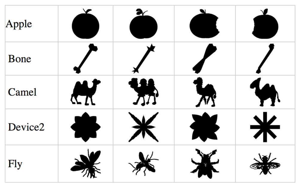
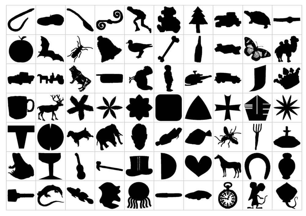
While FPFT is capable of extracting features that are invariant under rotation and translation, the peculiar distortions that affect silhouettes of 3-D objects are substantially different. This phenomenon is illustrated in Figure 11, which shows four sample shapes out of 20, selected from five of the 70 classes represented in the MPEG-7 CE-Shape-1 database used in our experiments (Figure 10). Besides undergoing arbitrarily scaling, translation and rotation, shapes belonging to the same class may be captured from independent instances of an object, possibly containing unique variations that may look different in ways that are hard to describe by mean of a simple transformation. RBRC retrieval begins with the feature extraction technique presented in the FPFT method.
Figure 10. MPEG-7 CE-Shape-1 database, one sample image from each of 70 classes.
Algorithms 05 00001 g010
Figure 11. Four sample shapes from five of the classes of the MPEG-7 CE-Shape-1 database.
Algorithms 05 00001 g011
First, a two-dimensional Fourier transform is applied to the original image. The output of the transform produces a stage-2 image composed of the magnitude of the Fourier coefficients. This step introduces invariance to translation in the case that the shape is not completely centered in the window. The stage-2 image is then transformed into polar coordinates, producing a stage-3 image. The coordinates of the polar transform are defined relative to the center of the window, which is why the translation invariance introduced by the Fourier transform is important.
With the image so transformed, a rotation of the input image produces an output image that is translated rather than rotated. The effect of this translation can be eliminated by again applying the translation-invariant Fourier transform, to produce a stage-4 image.
The two-dimensional result is then linearized and treated as a one-dimensional feature vector that constitutes the shape descriptor. Because this feature vector may be large, in our experiments we have reduced its dimensionality by using Fisher’s discriminants. Fisher’s discriminants maximize the separation between the classes while minimizing overlap between them. By measuring the discriminative power of each feature, the dimensions that do not help with the classification can be safely discarded.
One major difference between how FPFT is used on textures (Di Lillo, Motta, and Storer [16]) and how it is used here in the RBRC algorithm is that in the case of textured images, features were extracted on a pixel-by-pixel basis. In the case of a shape, the FPFT is computed once for the whole input image.
After shape images have been classified they are retrieved using a supervised approach, that is, a classifier is first trained, and then tested. Feature vectors are extracted as described above, one vector per sample image, and classified using a vector quantizer. Training extracts a small set of significant and discriminating features from shape images. The features extracted characterize the training samples. The basis for the classification consists of a set of h features extracted from n training images, which are formed by shapes belonging to k different classes.
Training our classifier consists of finding, for each class, a small set of “typical” feature vectors that, during the classification, are compared to an unknown signature to determine the class to which it belongs. We employ a vector quantizer, and for each class, determine a small set of centroids. Centroids are computed independently for each class, so that they minimize the mean squared error (MSE) with the feature vectors collected from the sample shapes.
To classify an unknown shape image, we extract its signature and compare it to the c × k centroids (c centroids for each of the k classes). The class associated with the centroid that is closest (in the Euclidean space) to the signature is finally assigned to the shape. As shall be seen in the next section, a small number is sufficient to fully characterize a class.
The RBRC algorithm has been tested on the MPEG-7 CE-Shape-1 database (Latecki, Lakamper, and Eckhardt [17]), a reference database widely used in literature that consists of 1400 silhouette images divided into 70 classes, each containing 20 images. Figure 10 shows a sample from each class. Shapes represented in this database may not only be rotated, but may also contain distortions such as occlusion and deformation. Furthermore, some classes contain objects whose shape is significantly different; an issue that is evident in the 20 images from 5 classes displayed in Figure 11.

4.2. Retrieval

Much of the existing literature assesses retrieval results with a method called the bull’s eye score. The bull’s eye score exemplifies the most typical use of a system that retrieves images based on their content. Given a query image, the N most similar images are retrieved from the database and the number of images belonging to the same class of the query is counted. After collecting the signatures for all shapes in a given class, as described in Section 3, a set of c centroids is determined. The process is repeated for each one of the 70 classes in the database determining in this way the c× 70 centroids. Then each of the 1400 images is used to query the database. The class of the query image is determined first. Independently of the fact that the class is correct or not, the c centroids corresponding to the class are used to retrieve N images that have minimum Euclidean distance with any of the c centroids. Finally, the number of images belonging to the original class of the query image is counted. The scores of the bull’s eye retrieval are compared in Table 1 with results in the existing literature.
For c = 6 centroids and N = 40, our method significantly improves upon the best result previously reported in the literature (93.06% as compared to 85.4%). It is noteworthy that the improvement achieved by the RBRC algorithm is based on feature extraction that also improves the state-of-the-art in both texture segmentation and classification. The feature extraction in FPFT proves to be a powerful representation of image features that can be used in RBRC to address a very different problem.
Table 1. Retrieval rate (bull’s eye measure, N = 40).
MethodScore
CSS (Mokhtarian, Abbasi, and Kittler [12])75.44%
Visual Parts (Latecki, Lakamper, and Eckhardt [17])76.45%
SC + TPS (Belongie, Malik, and Puzicha [14])76.51%
Curve Edit (Sebastian, Klein, and Kimia [18])78.71%
Distance Set (Grigorescu and Petkov [19])78.38%
MCSS (Jalba, Wilkinson, and Roerdink [20])78.80%
Generative Models (Tu and Yuille [21])80.03%
MDS + SC + DP (Ling and Jacobs [15])84.35%
IDSC + DP (Ling and Jacobs [15])85.40%
RBRC, c = 693.06%
Table 1 reports results for N = 40; that is, the number of correct shapes out of the top 40 retrieved. The choice of N = 40 is natural for the MPEG-7 CE-Shape-1 database because it is twice the number of shapes in each class, allowing for a reasonable but not overly large number returned for a given query (40) as compared to the maximum possible number of correct answers for a given query (20). Although N = 40 is the standard used in literature, it is worthwhile to note that performance of RBRC changes gracefully with N. In fact even at N = 20, RBRC about equals the best of the past results shown in Table 1 that use N = 40. Table 2 shows these results, with the top row having the value of N and the bottom row showing the percent success when the number of correct classification out of the top N retrieved is counted.
Table 2. RBRC retrieval rate (%) for different parameters N.
202530354045505560
88.290.588.790.393.193.593.994.394.4

4.3. Separation of Training from Testing

Experiments presented thus far have queried each image in the database against all others in order to compute statistics, which allows us to directly compare our results to those reported in literature. However, it is useful to ask how the training and testing of the system on the same sample shapes affects the results of classification and retrieval.
Table 3 presents experiments to address this question. In these experiments, the database is divided into two halves, each containing 10 shapes for each of the 70 classes (the first half contains shapes numbered from 1 to 10, the second the shapes numbered 11 to 20). The results are determined by first calculating the centroids from one half of the database, followed by testing the method on the other half. Table 3 shows both training of the first half and retrieval on the second, and vice-versa. As can be seen from Table 3, the bull’s eye retrieval is essentially unaffected when using only half of the database for training (still over 91%). This is further evidence of the robustness of RBRC.
Table 3. RBRC retrieval rate when testing on half of the database.
Train1st half1st half2nd half2nd half
Test1st half2nd half1st half2nd half
Score94.47%94.30%92.06%91.09%

4.4. Robustness to Rotation and Scaling

Robustness to rotation and scaling is an important property for a shape descriptor. We have tested RBRC for rotation and scale invariance by performing the experiments as specified in the MPEG-7 document (Jeannin and Bober [22]). Two new additional databases were constructed each containing 420 silhouette images; 70 of them are the reference shapes (one from each class of the original database) and the others are the derived shapes. The derived shapes in the rotation database were obtained by digitally rotating the basic shapes by 9°, 36°, 45° (composed of 9° and 36° rotations), 90° and 150°. For the scaling database, the derived shapes were obtained by reducing the basic shapes in each dimension by factors 0.3, 0.25, 0.2 and 0.1, and enlarged by a factor of 2. In these experiments, each silhouette is matched against all others and the performance is reported in terms of the top six retrieved images. Since the maximum number of corrected matches for a single query shape is 6, the maximum number of corrected matches is 2520. Table 4 shows the results obtained. Note that achieving scale invariance is more challenging then rotation invariance since some images are severely distorted when scaled by factors of 0.1 and 0.2.
Table 4. Results for rotation and scale invariance.
MethodRotationScalingAverage
Visual Parts (Latecki, Lakamper, and Eckhardt [17])100%88.65%94.33%
CSS (Mokhtarian, Abbasi, and Kittler [12])99.37%89.76%94.57%
Wavelets (Chuang and Kuo [23])97.46%88.04%92.75%
Zernike Moments (Khotanzan and Hong [24])99.60%92.54%96.07%
Multilayer Eigenvectors100%92.42%96.21%
(Latecki, Lakamper, and Eckhardt [17], Hyundai [25])
RBRC 99.52%93.02%96.27%

5. Location

There has been considerable past work on location with respect to a database. For example, Zamir and Shah [26] use a search-tree method to match a query image to its nearest match in the set of Google Street View images, Zhang and Kosecka [27] use a voting scheme to do an initial matching between the query image and the database followed by motion estimation to determine the exact location of the query image, and Teller et al. [28] describe a dataset of accurately geo-referenced images including camera calibration, taken on part of the MIT campus. We address a somewhat different model where we begin with approximate knowledge of our location from the most recently available GPS data to determine which images of the database are most relevant. Google Street View is perhaps the most well-known and well-developed database of this type. It provides 360-degree view images taken from a vehicle at intervals while traveling along city streets, along with location coordinates of where an image was acquired (given as [longitude, latitude]).
We have developed two location tools, the first being the tagging of database images. In a preprocessing phase (that is done only once at image acquisition time) a set of standard SIFT key points (e.g., Lowe [29]) is calculated for each relevant database image, and then a small set of corresponding points in two overlapping database images (e.g., successive images in Google Street View) are identified. The intersection of the two lines of sight from the acquisition coordinates to a pair of corresponding key points provides their coordinates. Appropriate ranking and weighted averaging of matching pairs can be used to refine accuracy and confidence.
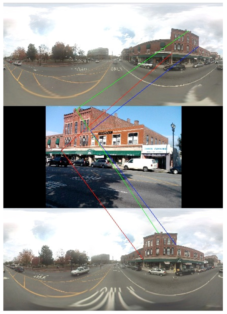
Figure 12. Location with respect to Google Street View database.
Algorithms 05 00001 g012
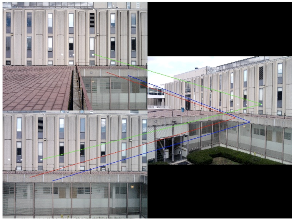
The preprocessing step creates geo-located key points along with their associated SIFT descriptors. When a user image has at least three points that can be matched with these database key points, a resection procedure like that used in land surveying can be employed: that is, from the apparent angles between these three points, as seen by the user, and the (already computed) locations of the points, we compute the location of the user. In Figure 12, the top and bottom images are two images from the Google Street View database, and the middle image is the user image. Figure 13 contains three images taken with a cell phone camera in a crowded area of buildings, where the two images on the left are database images, and the image on the right is the user’s view. Using the minimum number of three matched key points, we can predict the location of the user to within a couple of feet. When there are more matches available, there is an opportunity to improve accuracy by weighting and averaging multiple predictions.
Figure 13. Location with respect to campus database.
Algorithms 05 00001 g013

6. Conclusions and Current Research

We have presented basic tools for location with respect to an image database for subsequent application of (location informed) image segmentation and object recognition. In addition to improvement of our location tools (including improved initial accuracy by ranking and averaging of multiple matches), our current research seeks to take advantage of the knowledge static scene content based on the identified location in the image database (and the resulting identification of specific small sets of objects that are relevant to the task at hand) to enhance the accuracy of object recognition. A key application is navigation in urban environments for individuals who are visually impaired, where object recognition is otherwise difficult or not possible.

References

  1. Daptardar, A.; Storer, J.A. VQ Based Image Retrieval Using Color and Position Features. In Proceedings of the Data Compression Conference, Snowbird, UT, USA, 25-27 March 2008; pp. 432–441.
  2. Shapira, D.; Storer, J.A. In-Place Differential File Compression of Non-Aligned Files With Applications to File Distribution, Backups, String Similarity. In Proceedings of the Data Compression Conference, Snowbird, UT, USA, 23-25 March 2004; pp. 82–91.
  3. Shapira, D.; Storer, J.A. In-place differential file compression. Comput. J. 2005, 48, 677–691. [Google Scholar] [CrossRef]
  4. Jeong, S.; Gray, R.M. Minimum Distortion Color Image Retrieval Based on Lloyd-Clustered Gauss Mixtures. In Proceedings of the IEEE Data Compression Conference, Snowbird, UT, USA, 29-31 March 2005; pp. 279–288.
  5. Wyszecki, G.; Stiles, W.S. Color Science: Concepts and Methods, Quantitative Data and Formulae, 2nd ed; Wiley: Hoboken, NJ, USA, 2000. [Google Scholar]
  6. Gersho, A.; Gray, R.M. Vector Quantization and Signal Compression; Springer: Berlin, Germany, 1992. [Google Scholar]
  7. Jeong, S.; Won, C.S.; Gray, R.M. Histogram-Based Image Retrieval using Gauss Mixture Vector Quantization. In Proceedings of the 2003 International Conference on Multimedia and Expo, (ICME’03), Baltimore, MD, USA, 6-9 July 2003; 94, pp. 44–66.
  8. Wang, J. Semantics-sensitive Integrated Matching for Picture Libraries. Available online: http://wang.ist.psu.edu/cgi-bin/zwang/regionsearch_show.cgi (accessed on 9 January 2012).
  9. DiLillo, A.; Motta, G.; Storer, J.A. Texture Classification Based on Discriminative Features Extracted in the Frequency Domain. In Proceedings of the IEEE International Conference on Image Processing (ICIP), San Antonio, Texas, USA, 16-19 September 2007; pp. 53–56.
  10. Ojala, T.T.; Mäenpää, T.; Pietikäinen, M.; Viertola, J.; Kyllönen, J.; Huovinen, S. Outex-New Framework for Empirical Evaluation of Texture Analysis Algorithms. In Proceedings of the 16th International Conference on Pattern Recognition, Quebec, Canada, 11-15 August 2002; 1, pp. 701–706.
  11. Bober, M. MPEG-7 visual shape descriptors. IEEE Trans. Circuits Syst. Video Technol. 2001, 11, 716–719. [Google Scholar] [CrossRef]
  12. Mokhtarian, F.; Abbasi, S.; Kittler, J. Efficient and Robust Retrieval by Shape Content through Curvature Scale Space. In Image Databases and Multi-Media Search; Smeulders, A.W.M., Jain, R., Eds.; World Scientific: Singapore, 1997; pp. 51–58. [Google Scholar]
  13. Latecki, L.J.; Lakämper, R. Shape similarity measure based on correspondence of visual parts. IEEE Trans. Pattern Anal. Mach. 2000, 22, 1185–1190. [Google Scholar] [CrossRef]
  14. Belongie, S.; Malik, J.; Puzicha, J. Shape matching and object recognition using shape context. IEEE Trans. Pattern Anal. Mach. Intell. 2002, 24, 509–522. [Google Scholar] [CrossRef]
  15. Ling, H.; Jacobs, D.W. Shape classification using the inner-distance. IEEE Trans. Pattern Anal. Mach. Intell. 2007, 29, 286–299. [Google Scholar] [CrossRef]
  16. Di Lillo, A.; Motta, G.; Storer, J.A. Multiresolution Rotation-Invariant Texture Classification Using Feature Extraction in the Frequency Domain and Vector Quantization. In Proceedings of the Data Compression Conference, Snowbird, UT, USA, 25-27 March 2008; pp. 452–461.
  17. Latecki, L.J.; Lakamper, R.; Eckhardt, U. Shape Descriptors for Non-Rigid Shapes with a Single Closed Contour. In Proceedings of the IEEE Conference on Computer Vision and Pattern Recognition, Hilton Head Island, SC, USA, 13-15 June 2000; I, pp. 424–429.
  18. Sebastian, T.; Klein, P.; Kimia, B. On aligning curves. IEEE Trans. Pattern Anal. Mach. Intell. 2003, 25, 116–125. [Google Scholar] [CrossRef]
  19. Grigorescu, C.; Petkov, N. Distance sets for shape filters and shape recognition. IEEE Trans. Image Process. 2003, 12, 1274–1286. [Google Scholar] [CrossRef]
  20. Jalba, C.; Wilkinson, M.H.F.; Roerdink, J.B.T.M. Shape representation and recognition through morphological curvature scale spaces. IEEE Trans. Image Process. 2006, 15, 331–341. [Google Scholar] [CrossRef]
  21. Tu, Z.; Yuille, A.L. Shape Matching and Recognition-Using Generative Models and Informative Features. In Proceedings of the European Conference on Computer Vision, Prague, Czech Republic, 11-14 May 2004; 3, pp. 195–209.
  22. Jeannin, S.; Bober, M. Shape Matching and Recognition-Using Generative Models and Informative Features. In Description of core experiments for MPEG-7 motion/shape; ISO/IEC JTC1/SC29/WG11 /MPEG99/N2690; MPEG-7: Seoul, Korea, 03 1999. [Google Scholar]
  23. Chuang, C.; Kuo, C.-C. Wavelet descriptor of planar curves: Theory and applications. IEEE Trans. Image Process. 1996, 5, 56–70. [Google Scholar] [CrossRef]
  24. Khotanzan, A.; Hong, Y.H. Invariant image recognition by zernike moments. IEEE Trans. PAMI 1990, 12, 489–497. [Google Scholar] [CrossRef]
  25. Hyundai Electronics Industries Co., Ltd. Available online: http://www.wtec.org/loyola/satcom2/d_03.htm (accessed on 10 January 2012).
  26. Zamir, A.R.; Shah, M. Shah, M. Accurate Image Localization Based on Google Maps Street View. In Proceedings of the European Conference on Computer Vision (ECCV’10), Hersonissos, Heraklion, Crete, Greece, 5–11 September 2010.
  27. Zhang, W.; Kosecka, J. Image Based Localization in Urban Environments. In Proceedings of the 3rd International Symposium on 3D Data Visualization, and Transmission, Chapel Hill, NC, USA, 14–16 June 2006.
  28. Teller, S.; Antone, M.; Bodnar, Z.; Bosse, M.; Coorg, S.; Jethwa, M.; Master, N. Calibrated, registered images of an extended urban area. Int. J. Comput. Vis. 2003, 53, 93–107. [Google Scholar] [CrossRef]
  29. Lowe, D.G. Object Recognition from Local Scale-Invariant Features. In Proceedings of the 7th IEEE International Conference on Computer Vision, Kerkyra, Greece, 20-27 September 1999; pp. 1–8.