Linear-Time Text Compression by Longest-First Substitution

Abstract
:1. Introduction
Related Work
2. Preliminaries
2.1. Notations

2.2. Data Structures
3. Off-Line Compression by Longest-First Substitution
3.1. How to Find Using
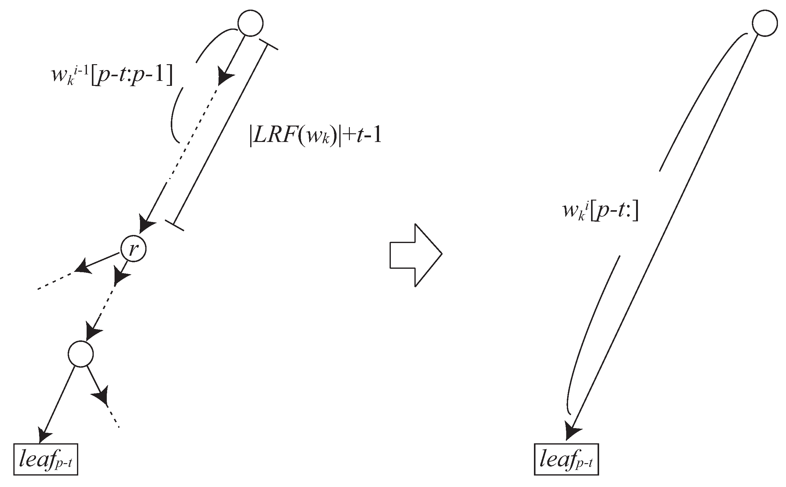
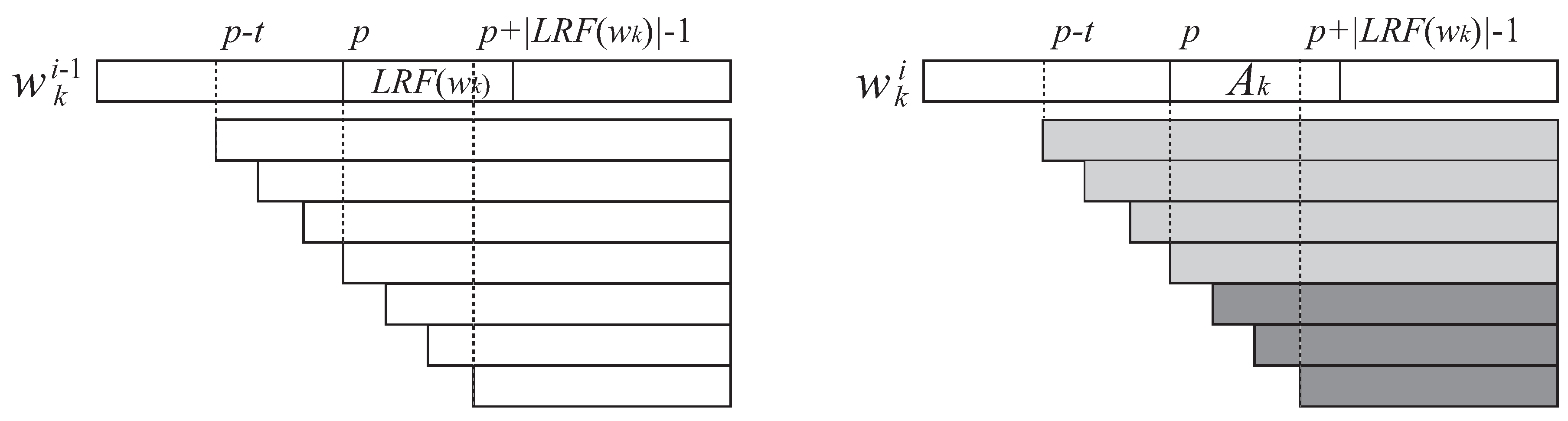
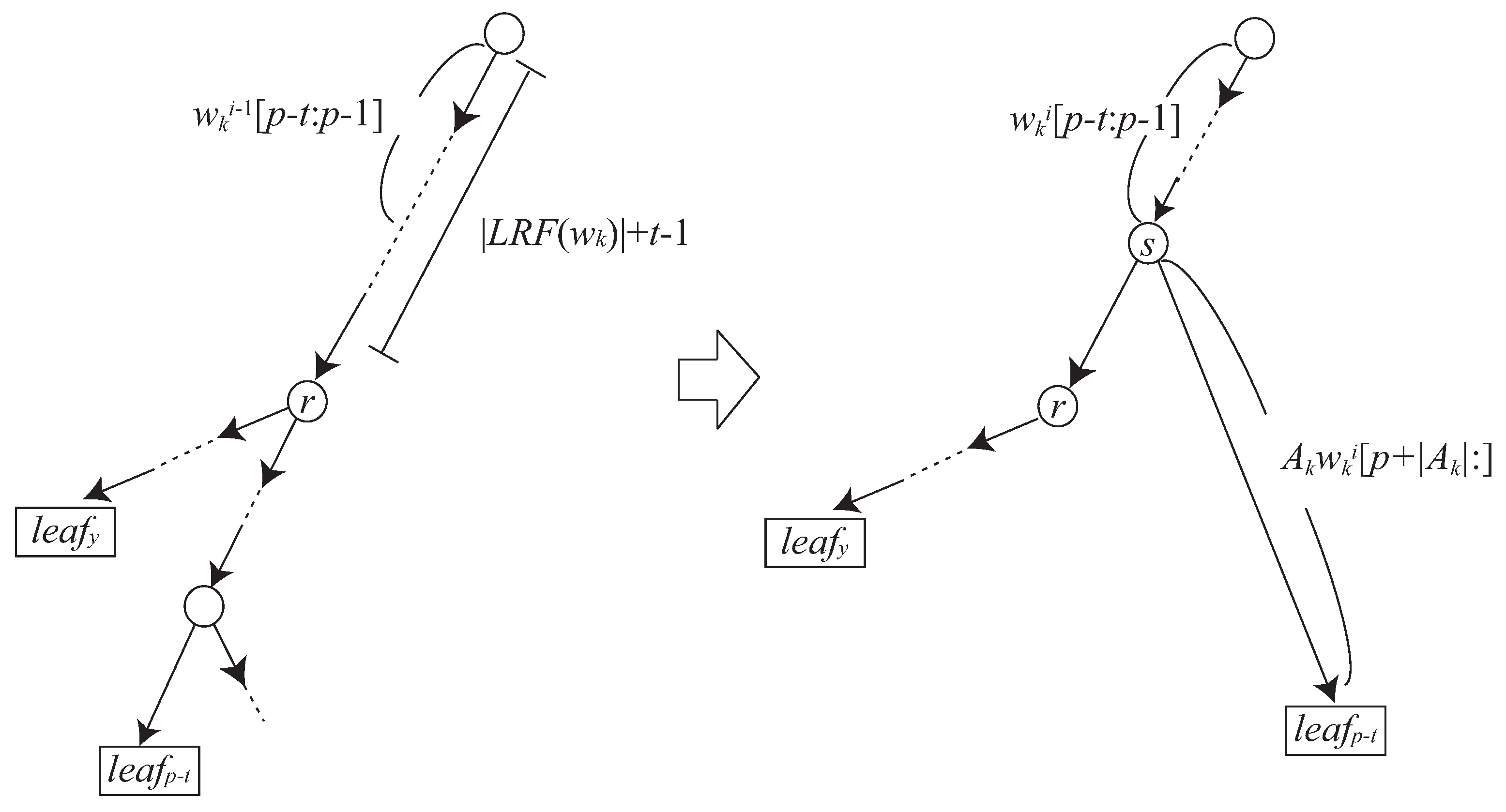
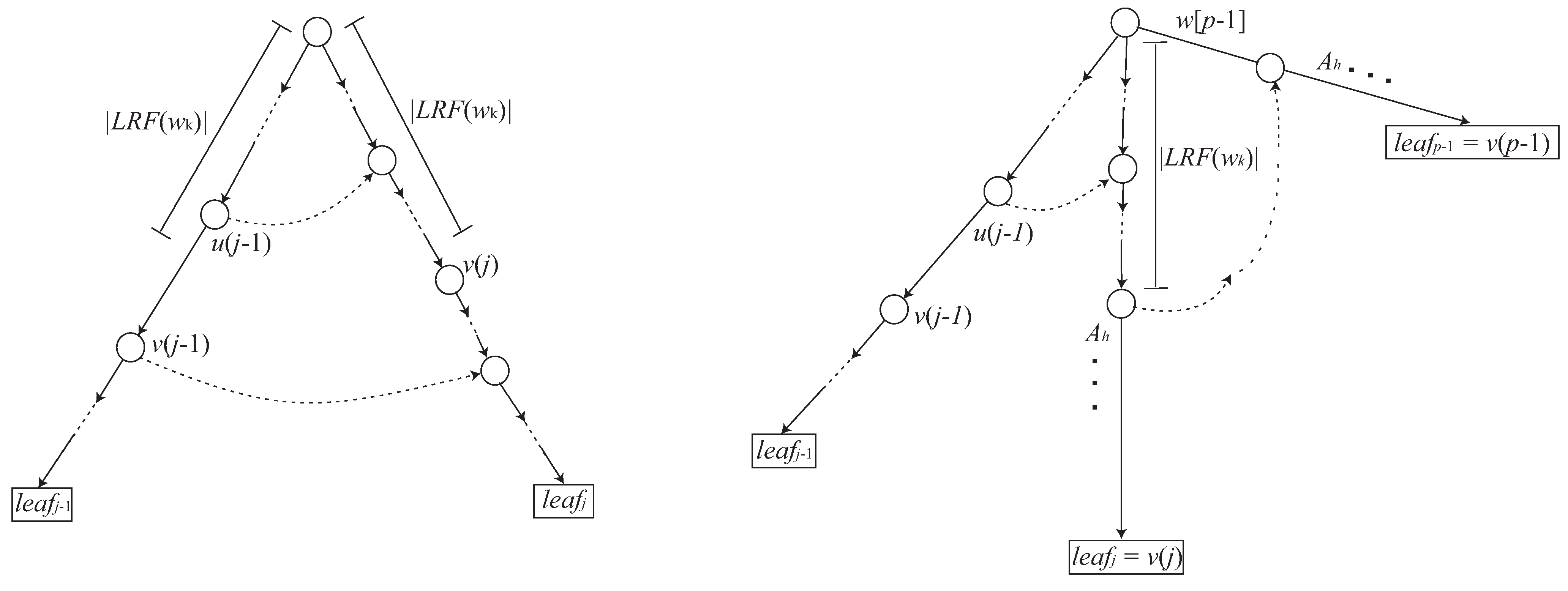
3.2. How to Update to
- If , then there exists an edge in from the root node to labeled with .
- If , then there exists a node s in such that and s has an edge labeled with and leading to .


3.3. Reducing Grammar Size
| Algorithms 1: Recursively find longest repeating factors. |
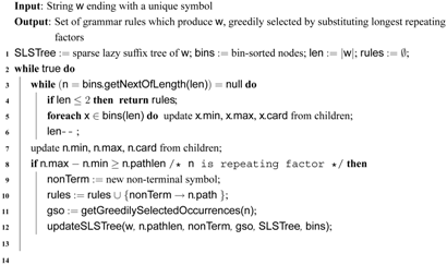 |
| Algorithm 2: updateSLSTree |
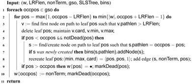 |
| Algorithm 3: getGreedilySelectedOccurrences |
 |
4. Conclusions and Future Work
Acknowledgments
References
- Kida, T.; Matsumoto, T.; Shibata, Y.; Takeda, M.; Shinohara, A.; Arikawa, S. Collage system: a unifying framework for compressed pattern matching. Theoretical Computer Science 2003, 298, 253–272. [Google Scholar] [CrossRef]
- M¨akinen, V.; Ukkonen, E.; Navarro, G. Approximate Matching of Run-Length Compressed Strings. Algorithmica 2003, 35, 347–369. [Google Scholar] [CrossRef]
- Lifshits, Y. Processing Compressed Texts: A Tractability Border. In Proc. 18th Annual Symposium on Combinatorial Pattern Matching (CPM’07); Springer-Verlag, 2007; Vol. 4580, Lecture Notes in Computer Science; pp. 228–240. [Google Scholar]
- Matsubara, W.; Inenaga, S.; Ishino, A.; Shinohara, A.; Nakamura, T.; Hashimoto, K. Efficient Algorithms to Compute Compressed Longest Common Substrings and Compressed Palindromes. Theoretical Computer Science 2009, 410, 900–913. [Google Scholar] [CrossRef]
- Hermelin, D.; Landau, G. M.; Landau, S.; Weimann, O. A Unified Algorithm for Accelerating Edit-Distance Computation via Text-Compression. In Proc. 26th International Symposium on Theoretical Aspects of Computer Science (STACS’09); 2009; pp. 529–540. [Google Scholar]
- Matsubara, W.; Inenaga, S.; Shinohara, A. Testing Square-Freeness of Strings Compressed by Balanced Straight Line Program. In Proc. 15th Computing: The Australasian Theory Symposium (CATS’09); Australian Computer Society, 2009; Vol. 94, CRPIT; pp. 19–28. [Google Scholar]
- Nevill-Manning, C. G.; Witten, I. H. Identifying hierarchical structure in sequences: a linear-time algorithm. J. Artificial Intelligence Research 1997, 7, 67–82. [Google Scholar]
- Nevill-Manning, C. G.; Witten, I. H. Online and offline heuristics for inferring hierarchies of repetitions in sequences. Proc. IEEE 2000, 88, 1745–1755. [Google Scholar] [CrossRef] [Green Version]
- Giancarlo, R.; Scaturro, D.; Utro, F. Textual data compression in computational biology: a synopsis. Bioinformatics 2009, 25, 1575–1586. [Google Scholar] [CrossRef] [PubMed]
- Kieffer, J. C.; Yang, E.-H. Grammar-based codes: A new class of universal lossless source codes. IEEE Transactions on Information Theory 2000, 46, 737–754. [Google Scholar] [CrossRef]
- Storer, J. NP-completeness Results Concerning Data Compression. Technical Report 234, Department of Electrical Engineering and Computer Science, Princeton University. 1977. [Google Scholar]
- Ziv, J.; Lempel, A. Compression of individual sequences via variable-rate coding. IEEE Trans. Information Theory 1978, 24, 530–536. [Google Scholar] [CrossRef]
- Welch, T. A. A Technique for High-Performance Data Compression. IEEE Computer 1984, 17, 8–19. [Google Scholar] [CrossRef]
- Kieffer, J. C.; Yang, E.-H.; Nelson, G. J.; Cosman, P. C. Universal lossless compression via multilevel pattern matching. IEEE Transactions on Information Theory 2000, 46, 1227–1245. [Google Scholar] [CrossRef]
- Sakamoto, H. A fully linear-time approximation algorithm for grammar-based compression. Journal of Discrete Algorithms 2005, 3, 416–430. [Google Scholar] [CrossRef]
- Rytter, W. Application of Lempel-Ziv factorization to the approximation of grammar-based compression. Theoretical Computer Science 2003, 302, 211–222. [Google Scholar] [CrossRef]
- Sakamoto, H.; Maruyama, S.; Kida, T.; Shimozono, S. A Space-Saving Approximation Algorithm for Grammar-Based Compression. IEICE Trans. on Information and Systems 2009, E92-D, 158–165. [Google Scholar] [CrossRef]
- Maruyama, S.; Tanaka, Y.; Sakamoto, H.; Takeda, M. Context-Sensitive Grammar Transform: Compression and Pattern Matching. In Proc. 15th International Symposium on String Processing and Information Retrieval (SPIRE’08); Springer-Verlag, 2008; Vol. 5280, Lecture Notes in Computer Science; pp. 27–38. [Google Scholar]
- Wolff, J. G. An algorithm for the segmentation for an artificial language analogue. British Journal of Psychology 1975, 66, 79–90. [Google Scholar] [CrossRef]
- Larsson, N. J.; Moffat, A. Offline Dictionary-Based Compression. In Proc. Data Compression Conference ’99 (DCC’99); IEEE Computer Society, 1999; p. 296. [Google Scholar]
- Apostolico, A.; Lonardi, S. Off-Line Compression by Greedy Textual Substitution. Proc. IEEE 2000, 88, 1733–1744. [Google Scholar] [CrossRef]
- Apostolico, A.; Lonardi, S. Compression of Biological Sequences by Greedy Off-Line Textual Substitution. In Proc. Data Compression Conference ’00 (DCC’00); IEEE Computer Society, 2000; pp. 143–152. [Google Scholar]
- Ziv, J.; Lempel, A. A Universal Algorithm for Sequential Data Compression. IEEE Transactions on Information Theory 1977, IT-23, 337–349. [Google Scholar] [CrossRef]
- Burrows, M.; Wheeler, D. A block sorting lossless data compression algorithm. Technical Report 124, Digital Equipment Corporation. 1994. [Google Scholar]
- Nakamura, R.; Bannai, H.; Inenaga, S.; Takeda, M. Simple Linear-Time Off-Line Text Compression by Longest-First Substitution. In Proc. Data Compression Conference ’07 (DCC’07); IEEE Computer Society, 2007; pp. 123–132. [Google Scholar]
- Inenaga, S.; Funamoto, T.; Takeda, M.; Shinohara, A. Linear-time off-line text compression by longest-first substitution. In Proc. 10th International Symposium on String Processing and Information Retrieval (SPIRE’03); Springer-Verlag, 2003; Vol. 2857, Lecture Notes in Computer Science; pp. 137–152. [Google Scholar]
- Bentley, J.; McIlroy, D. Data compression using long common strings. In Proc. Data Compression Conference ’99 (DCC’99); IEEE Computer Society, 1999; pp. 287–295. [Google Scholar]
- Lanctot, J. K.; Li, M.; Yang, E.-H. Estimating DNA sequence entropy. In Proc. 11th Annual ACM-SIAM Symposium on Discrete Algorithms (SODA’00); 2000; pp. 409–418. [Google Scholar]
- Ukkonen, E. On-line Construction of Suffix Trees. Algorithmica 1995, 14, 249–260. [Google Scholar] [CrossRef]
- K¨arkk¨ainen, J.; Ukkonen, E. Sparse Suffix Trees. In Proc. 2nd Annual International Computing and Combinatorics Conference (COCOON’96); Springer-Verlag, 1996; Vol. 1090, Lecture Notes in Computer Science; pp. 219–230. [Google Scholar]
- Apostolico, A.; Preparata, F. P. Data structures and algorithms for the string statistics problem. Algorithmica 1996, 15, 481–494. [Google Scholar] [CrossRef]
- Brødal, G. S.; Lyngsø, R. B.; O¨stlin, A.; Pedersen, C. N. S. Solving the String Stastistics Problem in Time O(n log n). In Proc. 29th International Colloquium on Automata,Languages, and Programming (ICALP’02); Springer-Verlag, 2002; Vol. 2380, Lecture Notes in Computer Science; pp. 728–739. [Google Scholar]
- Lanctot, J. K. Some String Problems in Computational Biology. PhD thesis, University ofWaterloo, 2004. [Google Scholar]
Appendix
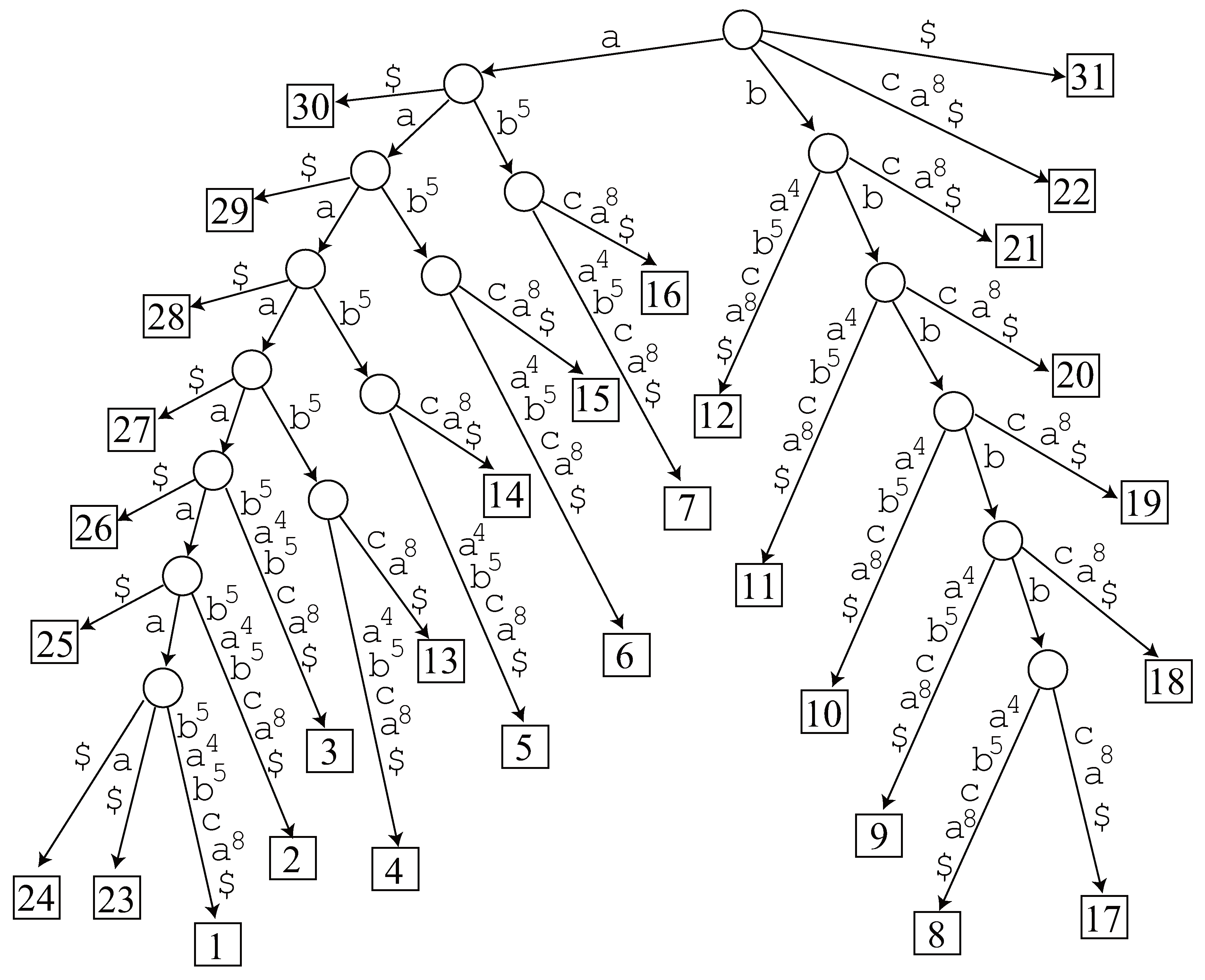
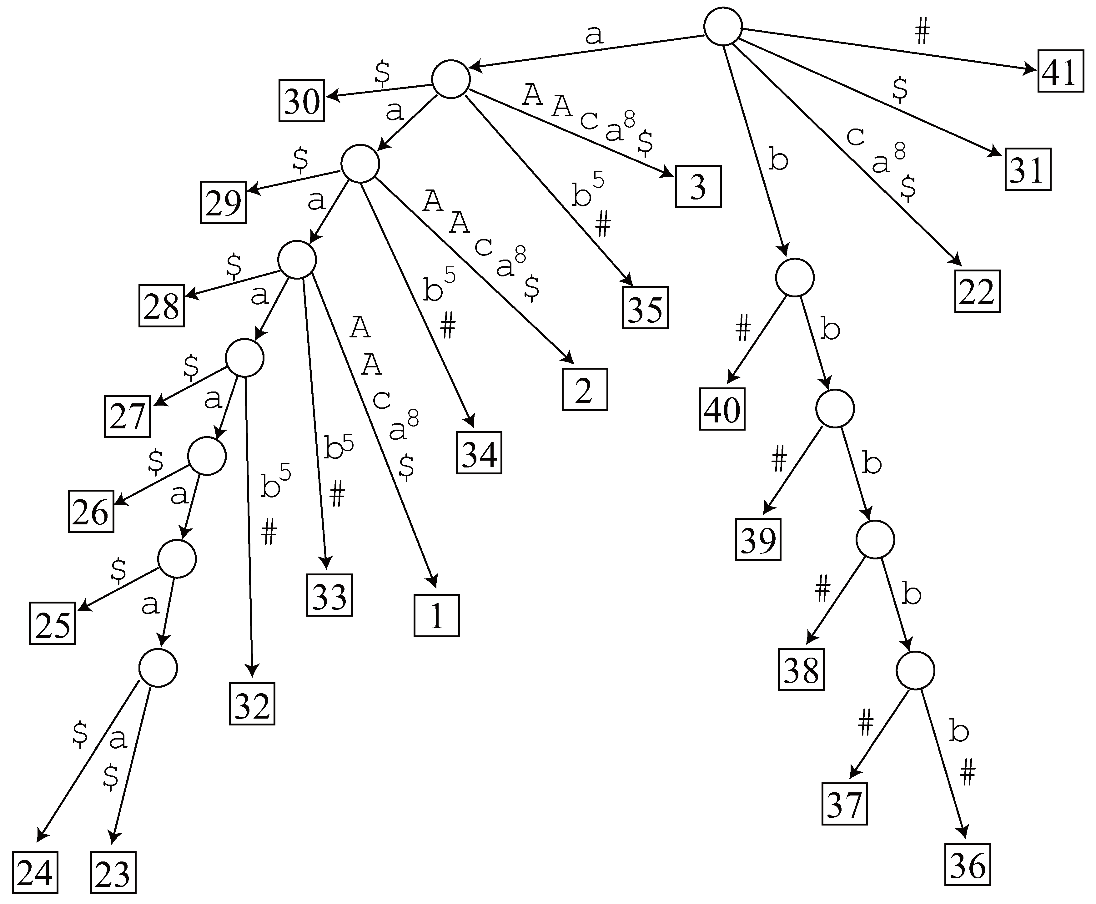
- Length 8. The generalized suffix tree has no node representing , and hence it is not an LRF.
- Length 7. Since node exists in the generalized suffix tree, we traverse its subtree and find 2 occurrences 23 and 24 in . However, it is not an LRF of . The other candidate does not have a corresponding node in the tree, so it is not an LRF, either.
- Length 6. Node exists in the generalized suffix tree and we find 3 occurrences 23, 24 and 25 in by traversing the tree, but it is not an LRF. The tree has no node corresponding to , hence it is not an LRF.
- Length 5. Node exists in the generalized suffix tree and we find 4 occurrences 23, 24, 25 and 26 in by traversing the tree, but it is not an LRF. There is no node in the tree corresponding to .

- Length 4. Node exists in the generalized suffix tree and we find 5 occurrences 23, 24, 25, 26 and 27. Now 23 and 27 are non-overlapping occurrences of , and hence it is an LRF of .
© 2009 by the authors; licensee Molecular Diversity Preservation International, Basel, Switzerland. This article is an open access article distributed under the terms and conditions of the Creative Commons Attribution license (http://creativecommons.org/licenses/by/3.0/).
Share and Cite
Nakamura, R.; Inenaga, S.; Bannai, H.; Funamoto, T.; Takeda, M.; Shinohara, A. Linear-Time Text Compression by Longest-First Substitution. Algorithms 2009, 2, 1429-1448. https://doi.org/10.3390/a2041429
Nakamura R, Inenaga S, Bannai H, Funamoto T, Takeda M, Shinohara A. Linear-Time Text Compression by Longest-First Substitution. Algorithms. 2009; 2(4):1429-1448. https://doi.org/10.3390/a2041429
Chicago/Turabian StyleNakamura, Ryosuke, Shunsuke Inenaga, Hideo Bannai, Takashi Funamoto, Masayuki Takeda, and Ayumi Shinohara. 2009. "Linear-Time Text Compression by Longest-First Substitution" Algorithms 2, no. 4: 1429-1448. https://doi.org/10.3390/a2041429
APA StyleNakamura, R., Inenaga, S., Bannai, H., Funamoto, T., Takeda, M., & Shinohara, A. (2009). Linear-Time Text Compression by Longest-First Substitution. Algorithms, 2(4), 1429-1448. https://doi.org/10.3390/a2041429