Abstract
We consider grammar-based text compression with longest first substitution (LFS), where non-overlapping occurrences of a longest repeating factor of the input text are replaced by a new non-terminal symbol. We present the first linear-time algorithm for LFS. Our algorithm employs a new data structure called sparse lazy suffix trees. We also deal with a more sophisticated version of LFS, called LFS2, that allows better compression. The first linear-time algorithm for LFS2 is also presented.
1. Introduction
Data compression is a task of reducing data description length. Not only does it enable us to save space for data storage, but also it reduces time for data communication. This paper focuses on text compression where the data to be compressed are texts (strings). Recent research developments show that text compression has a wide range of applications, e.g., pattern matching [1, 2, 3], string similarity computation [4, 5], detecting palindromic/repetitive structures [4, 6], inferring hierarchal structure of natural language texts [7, 8], and analyses of biological sequences [9].
Grammar-based compression [10] is a kind of text compression scheme in which a context-free grammar (CFG) that generates only an input text w is output as a compressed form of w. Since the problem of computing the smallest CFG which generates w is NP-hard [11], many attempts have been made to develop practical algorithms that compute a small CFG which generates w. Examples of grammar-based compression algorithms are LZ78 [12], LZW [13], Sequitur [7], and Bisection [14]. Approximation algorithms for optimal grammar-based compression have also been proposed [15, 16, 17]. The first compression algorithm based on a subclass of context-sensitive grammars was introduced in [18].
Grammar-based compression based on greedy substitutions has been extensively studied. Wolff [19] introduced a concept of most-frequent-first substitution (MFFS) such that a digram (a factor of length 2) which occurs most frequently in the text is recursively replaced by a new non-terminal symbol. He also presented an -time algorithm for it, where n is the input text length. A linear-time algorithm for most-frequent-first substitution, called Re-pair, was later proposed by Larsson and Moffat [20]. Apostolico and Lonardi [21] proposed a concept of largest-area-first substitution such that a factor of the largest “area” is recursively replaced by a new non-terminal symbol. Here the area of a factor refers to the product of the length of the factor by the number of its non-overlapping occurrences in the input text. It was reported in [22] that compression by largest-area-first substitution outperforms gzip (based on LZ77 [23]) and bzip2 (based on the Burrows-Wheeler Transform [24]) on DNA sequences. However, to the best of our knowledge, no linear-time algorithm for this compression scheme is known.
This paper focuses on another greedy text compression scheme called longest-first substitution (LFS), in which a longest repeating factor of an input text is recursively replaced by a new non-terminal symbol. For example, for input text , the following grammar
which generates only w is the output of LFS.
In this paper, we propose the first linear-time algorithm for text compression by LFS substitution. A key idea is the use of a new data structure called sparse lazy suffix trees. Moreover, this paper deals with a more sophisticated version of longest-first text compression (named LFS2), where we also consider repeating factors of the right-hand of the existing production rules. For the same input text as above, we obtain the following grammar:
This method allows better compression since the total grammar size becomes smaller. In this paper, we present the first linear-time algorithm for text compression based on LFS2. Preliminary versions of our paper appeared in [25] and [26].
Related Work
It is true that several algorithms for LFS or LFS2 were already proposed, however, in fact none of them runs in linear time in the worst case. Bentley and McIlroy [27] proposed an algorithm for LFS, but Nevill-Manning and Witten [8] pointed out that the algorithm does not run in linear time. Nevill-Manning and Witten also claimed that the algorithm can be improved so as to run in linear time, but they only noted a too short sketch for how, which is unlikely to give a shape to the idea of the whole algorithm. Lanctot et al. [28] proposed an algorithm for LFS2 and stated that it runs in linear time, but a careful analysis reveals that it actually takes time in the worst case for some input string of length n. See Appendix for our detailed analysis.
2. Preliminaries
2.1. Notations
Let Σ be a finite alphabet of symbols. We assume that Σ is fixed and is constant. An element of is called a string. Strings x, y, and z are said to be a prefix, factor, and suffix of string , respectively.
The length of a string w is denoted by . The empty string is denoted by , that is, . Also, we assume that all strings end with a unique symbol that does not occur anywhere else in the strings. Let . The i-th symbol of a string w is denoted by for , and the factor of a string w that begins at position i and ends at position j is denoted by for . For convenience, let for , and for . For any strings , let denote the set of the beginning positions of all the occurrences of x in w. That is, .
We say that strings overlap in w if there exist integers such that , , and or .
Let denote the possible maximum number of non-overlapping occurrences of x in w. If , then x is said to be repeating in w. We abbreviate a longest repeating factor of w to an LRF of w. Remark that there can exist more than one LRF for w.
Let Σ and Π be the set of terminal and non-terminal symbols, respectively, such that . A context-free grammar is a formal grammar in which every production rule is of the form , where and . Let and with and . If there exists a production rule in , then is said to be directly derived from by , and it is denoted by . If there exists a sequence such that and
then we say that v is derived from u. The length of a non-terminal symbol A, denoted , is the length of the string that is derived from the production rule . For convenience, we assume that any non-terminal symbol A in has positions. The size of the production rule is the number of terminal and non-terminal symbols v contains.
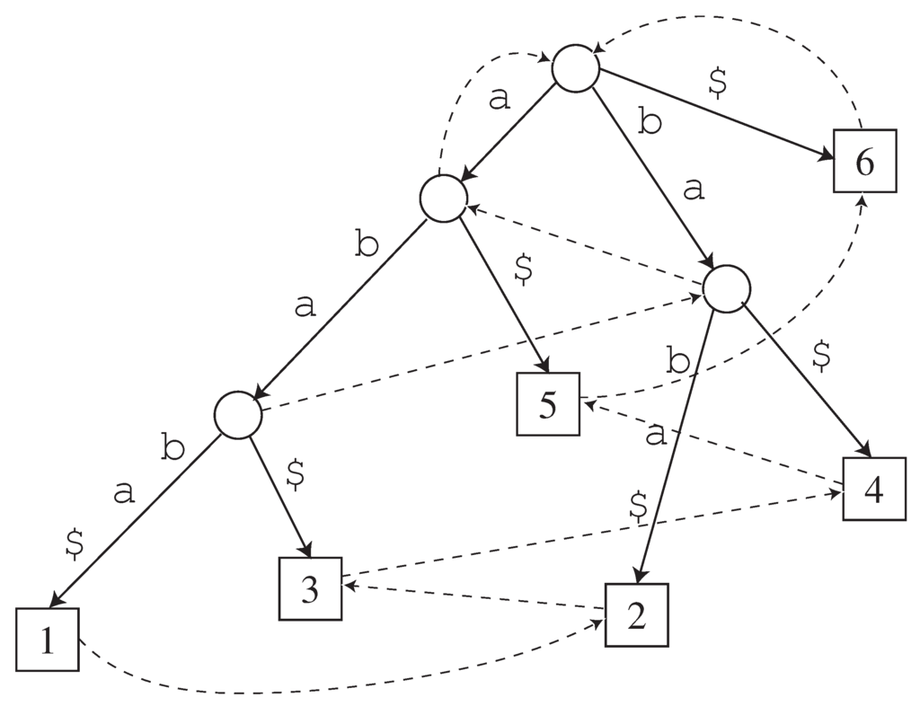
Figure 1.
with . Solid arrows represent edges, and dotted arrows are suffix links.
2.2. Data Structures
Our text compression algorithm uses a data structure based on suffix trees [29]. The suffix tree of string w, denoted by , is defined as follows:
Definition 1 (Suffix Trees)
is a tree structure such that: (1) every edge is labeled by a non-empty factor of w, (2) every internal node has at least two child nodes, (3) all out-going edge labels of every node begin with mutually distinct symbols, and (4) every suffix of w is spelled out in a path starting from the root node.
Assuming any string w terminates with the unique symbol $ not appearing elsewhere in w, there is a one-to-one correspondence between a suffix of w and a leaf node of . It is easy to see that the numbers of the nodes and edges of are linear in . Moreover, by encoding every edge label x of with an ordered pair of integers such that , each edge only needs constant space. Therefore, can be implemented with total of space. Also, it is well known that can be constructed in time (e.g. see [29]).
for string is shown in Figure 1. For any node v of , denotes the string obtained by concatenating the labels of the edges in the path from the root node to node v. The length of node v, denoted , is defined to be . It is an easy application of the Ukkonen algorithm [29] to compute the lengths of all nodes while constructing . The leaf node such that is denoted by , and i is said to be the id of the leaf. Every node v of except for the root node has a suffix link, denoted by , such that where is a suffix of and . Linear-time suffix tree construction algorithms (e.g., [29]) make extensive use of the suffix links.
A sparse suffix tree [30] of is a kind of suffix tree which represents only a subset of the suffixes of w. The sparse suffix tree of represents the subset of suffixes of w which begin with a terminal symbol. Let be the length of the LRFs of w. A reference node of the sparse suffix tree of is any node v such that , and there is no node u such that is a proper prefix of and .
Our algorithm uses the following data structure.
Definition 2 (Sparse Lazy Suffix Trees)
A sparse lazy suffix tree (SLSTree) of string , denoted by , is a kind of sparse suffix tree such that: (1) All paths from the root node to the reference nodes coincide with those of the sparse suffix tree of w, and (2) Every reference node v stores an ordered triple such that , , and .
is called “lazy” since its subtrees that are located below the reference nodes may not coincide with those of the corresponding sparse suffix tree of w. Our algorithms of Section 3. run in linear time by “neglecting” updating these subtrees below the reference nodes.
Proposition 1
For any string , can be obtained from in time.
Proof.
By a standard postorder traversal on , propagating the id of each leaf node. □
Since can be constructed in time [29], we can build in total of time.
3. Off-Line Compression by Longest-First Substitution
Given a text string , we here consider a greedy approach to construct a context-free grammar which generates only w. The key is how to select a factor of w to be replaced by a non-terminal symbol from Π. Here, we consider the longest-first-substitution approach where we recursively replace as many LRFs as possible with non-terminal symbols.
Example.
Let . At the beginning, the grammar is of the following simple form , where the right-hand of the production rule consists only of terminal symbols from Σ. Now we focus on the right-hand of S which has two LRFs and . Let us here choose to be replaced by non-terminal . We obtain the following grammar: ; . The other LRF of length 3 is no longer present in the right-hand of S. Thus we focus on an LRF of length 2. Replacing by non-terminal results in the following grammar: ; ; . Since the right-hand of S has no repeating factor longer than 1, we are done.
Let , and let denote the string obtained by replacing an LRF of with a non-terminal symbol . denotes the LRF of that is replaced by , namely, we create a new production rule . In the above example, , , , , , , and .
Due to the property of the longest first approach, we have the following observation.
Observation 1
Let be the non-terminal symbols which replace , respectively. For any , the right-hand of the production rule of contains none of .
In what follows, we will show our algorithm which outputs a context-free grammar which generates a given string. Our algorithm heavily uses the SLSTree structure.
3.1. How to Find Using
In this section, we show how to find an LRF of from .
The next lemmas characterize an LRF of that is not represented by a node of .
Lemma 1
If an LRF x of is not represented by a node of , then .
Proof.
Let and . Since x is a repeating factor of , , which means that . If , then it contradicts the precondition that x is not represented by a node of . Hence we have . Moreover, since x is an LRF of , we have . However, if we assume , this contradicts the precondition that x is an LRF of , since and we obtain a longer LRF . Hence we have . □
The above lemma implies that an LRF x is not represented by a node of only if the first and the last occurrences of x form a square in . For example, see Figure 1 that illustrates for . One can see that is an LRF of but it is not represented by a node of .
However, the following lemma guarantees that it is indeed sufficient to consider the strings represented by nodes of as candidates for .
Lemma 2
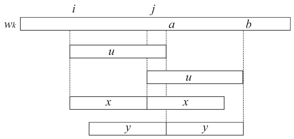
Let x be an LRF of that is not represented by a node of . Then, there exists another LRF y of that is represented by a node of such that . Moreover, x is no longer present in after a substitution for y (see also Figure 2).
Proof.
Let and . It follows from Lemma 1 that . Suppose that x is represented on an edge from some node s to some node t of . Let . Then we have . Let y be the suffix of u of length . It is clear that . Since , . Thus y is an LRF of . Since u is represented by node t and and , we know that . Hence y is represented by a node of . Since x occurs only within the region , x does not occur in after a substitution for y. □
In the running example of Figure 1, is an LRF of that is represented by a node of . After its two occurrences are replaced by a non-terminal symbol , then , which is an LRF of not represented by a node of , is no more present in .
After constructing , we create a bin-sorted list of the internal nodes of in the decreasing order of their lengths. This can be done in linear time by a standard
 traversal on . We remark that a new internal node v may appear in for some , which did not exist in . However, we have that . Thus, we can maintain the bin-sorted list by inserting node v in constant time.

Figure 2.
Illustration for proof of Lemma 2. Since u is represented by a node of , we know that .
Given a node s in the bin-sorted list, we can determine whether is repeating or not by using , as follows.
Lemma 3
Let s be any node of with and let be the children of s. Then is a disjoint union of .
Proof.
Clear from the definition of . □
Lemma 4
For any node s of such that , it takes amortized constant time to check whether or not is an LRF of .
Proof.
Let be the children of s. Then, is repeating if and only if
Remark that the values of and are stored in node and can be referred to in constant time. Since the above inequality is checked at most once for each node s, it takes amortized constant time. □
Suppose we have found an LRF of as mentioned above. In the sequel, we show our greedy strategy to select occurrences of the LRF in to be replaced with a new non-terminal symbol.
The next lemma is essentially the same as Lemma 2 of Kida et al. [1].
Lemma 5
For any non-repeating factor x of , forms a single arithmetic progression.
Therefore, for any non-repeating factor x of , can be expressed by an ordered triple consisting of minimum element , maximum element , and cardinality , which takes constant space.
Lemma 6
Let s be any node of such that is an LRF of , and be any child of s. Then, contains at most two positions corresponding to non-overlapping occurrences of in .
Proof.
Assume for contrary that contains three non-overlapping occurrences of , and let them be in the increasing order. Then we have
which implies that and are non-overlapping. Moreover, since , we have . However, this contradicts the precondition that is an LRF of . □
From Lemma 6, each child of node s such that is an LRF, corresponds to at most two non-overlapping occurrences of . Due to Lemma 3, we can greedily select occurrences of to be replaced by a new non-terminal symbol, by checking all children of node s. According to Lemma 5, it takes amortized constant time to select such occurrences for each node s.
Note that we have to select occurrences of so that no occurrences of remain in the text string, and at least two occurrences of are selected. We remark that we can greedily choose at least occurrences.
3.2. How to Update to
Let L be the set of the greedily selected occurrences of in . For any , let denote the string obtained after replacing the first i occurrences of with non-terminal symbol . Namely, and .
In this section we show how to update to . Let p be the beginning position of the i-th occurrence in L. Assume that we have , and that we have replaced with non-terminal symbol such that . We now have , and we have to update to .
A naive way to obtain is to remove all the suffixes of from and insert all the suffixes of into it. However, since only the nodes not longer than are important for our longest-first strategy, only the suffixes such that and for any have to be removed from , and only the suffixes have to be inserted into the tree (see the light-shaded suffixes of Figure 3).
Lemma 7
For any t, let r be the shortest node of such that is a prefix of . Assume .
- If , then there exists an edge in from the root node to labeled with .
- If , then there exists a node s in such that and s has an edge labeled with and leading to .
Proof.
Consider Case 1 (see also Figure 4). Since , . Hence is a non-repeating factor of . By Lemma 5, forms a single arithmetic progression. Also, since , . Therefore, if

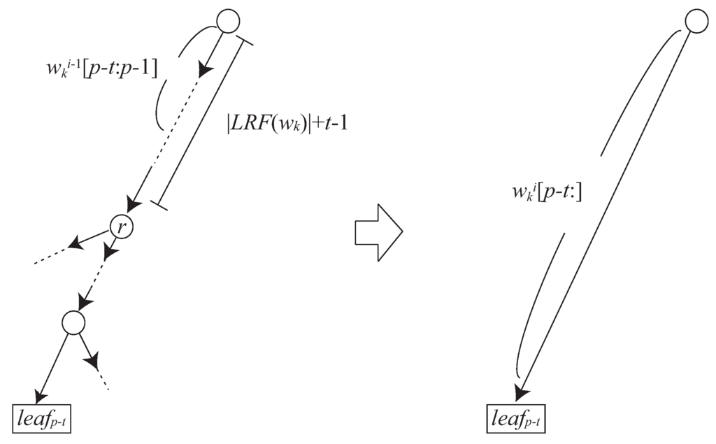 , then . Hence there exists an edge from the root node to labeled with in .

Figure 3.
at position p of is replaced by non-terminal symbol in . Every is removed from the tree and every is inserted into the tree (the light-shaded suffixes in the right figure). In addition, every for is removed from the tree (the dark-shaded suffixes in the right figure).

Figure 4.
Illustration of Case 1 of Lemma 7.
Consider Case 2 (see also Figure 5). Let . Then . Since , and since r is not longer than the reference node in the path spelling out from the root node of , there exists at least one integer m such that and . Hence there exists a node s in such that and has an out-going edge labeled with and leading to .□
It is not difficult to see that the edge in each case of Lemma 7 does not exist in . Hence we create the edge when we update to .
The next lemma states how to locate node s of Case 2 of Lemma 7.
Lemma 8
For each t, we can locate node s such that in amortized constant time.
Proof.
Let be the longest node in the tree such that is a prefix of .
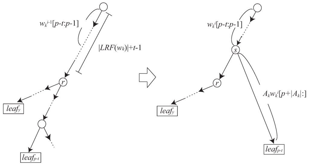
Figure 5.
Illustration of Case 2 of Lemma 7.
Consider the largest possible t and denote it by . Since , the node can be found in time by going down the path that spells out from the root node (recall that Σ is fixed). Let be the string such that . If , then we create a new child node of such that . Otherwise, we set .
Now assume that we have located nodes and . We can then locate as follows. Consider node . Remark that is a prefix of , and thus we can detect in time by using the suffix link. After finding , we can locate or create in constant time.
The total time cost for detecting for all is linear in
Hence we can locate each in amortized constant time. □
Let v be the reference node in the path from the root to some . Assume that is removed from the subtree of v, and redirected to node s in the same path, such that . In order to update to , we have to maintain triple for node v. One may be concerned that if is neither or and in
 , the occurrences of in do not form a single arithmetic progression any more. However, we have the following lemma. For any factor y of , let , namely, denotes the occurrences of y in that overlap with the i-th greedily selected occurrence of in .

Figure 6.
Illustration of proof for Lemma 9.
Lemma 9
Let v be any reference node of such that . For any integer , if , then there is no integer r such that and . (See Figure 6).
Proof.
Assume for contrary that there exists integer r such that and . Since , there exist integers such that , and . For any integer j such that and , we have . Since , . As is non-repeating, . Since , is a factor of . Therefore, there exist two integers such that . Since , is repeating and . It contradicts that is an LRF of . □
Recall that p is the beginning position of the i-th largest greedily selected occurrence of in . Also, for any such that for every , we have removed from the subtree rooted at the reference node v and have reconnected it to node s such that . According to the above lemma, if , for every is removed from the subtree of v. After processing , then is updated to where is the step of the progression, and is updated to .
Notice that for every has to be removed from the tree, since and therefore this leaf node should not exist in (see the dark-shaded suffixes of Figure 3). Removing each leaf can be done in constant time. Maintaining the information about the triple for the arithmetic progression of the reference nodes can be done in the same way as mentioned above.
The following lemma states how to locate each reference node.
Lemma 10
Let p be the i-th greedily selected occurrence of in . For any integer such that , let denote the reference node of in the path from the root spelling out suffix . For each j such that , we can locate the reference node in amortized constant time.
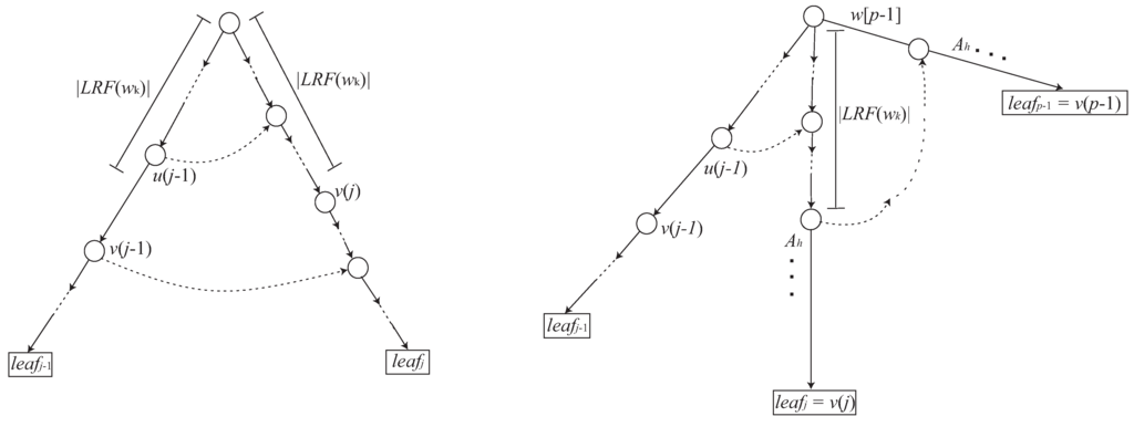
Figure 7.
The left figure illustrates how to find from . The right one illustrates a special case where . Once , it stands that for any .
Proof.
Let . We find by spelling out from the root in time, since there can be at most nodes in the path from the root to .
Suppose we have found . We find as follows. Let be the parent node of . We have and . We go to . Since , we have . Thus, we can find by going down the path starting from and spelling out . (See also the left illustration of Figure 7).
A special case happens when there exists a node s in the path from the root to , such that and the edge from s in the path starts with some non-terminal symbol with . Namely, . Due to the property of the longest first approach, we have . Thus . Moreover, for any , . (See also the right illustration of Figure 7). It is thus clear that each can be found in constant time. Since , the leaves corresponding to with do not exist in . □
From the above discussions, we conclude that:
Theorem 1
For any string , the proposed algorithm for text compression by longest first substitution runs in time using space.
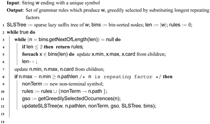
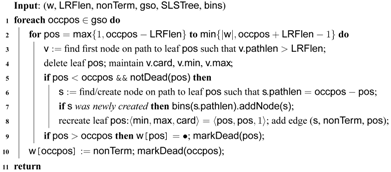
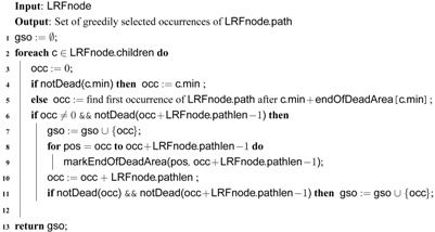
Pseudo-codes of our algorithms are shown in Algorithms 1, 2, and 3.
3.3. Reducing Grammar Size
In the above sections we considered text compression by longest first substitution, where we construct a context free grammar that generates only a given string w. By Observation 1, for any production rule of , contains only terminal symbols from Σ. In this section, we take the factors of into consideration for candidates of LRFs, and also replace LRFs appearing in . This way we can reduce
the total size of the grammar. In so doing, we consider an LRF of string , where and each appears nowhere else in .
| Algorithms 1: Recursively find longest repeating factors. |
 |
| Algorithm 2: updateSLSTree |
 |
| Algorithm 3: getGreedilySelectedOccurrences |
 |
Example.
Let . We replace an LRF with A, and obtain the following grammar: ; . Then, and . Now, . We replace an LRF of with a non-terminal B, getting ; ; . Then, and . Now, . Since there is no LRF of length more than 1 in , we are done.
We call this method of text compression LFS2.
Theorem 2
Given a string w, the LFS2 strategy compresses w in linear time and space.
Proof.
We modify the algorithm proposed in the previous sections. If we have a generalized SLSTree for set , of strings, we can find an LRF of . It follows from the property of the longest first substitution strategy that for any . Therefore, any new node inserted into the generalized SLSTree for , is shorter than the reference nodes of the tree. Thus, using the Ukkonen on-line algorithm [29], we can obtain the generalized SLSTree of , , by inserting the suffixes of each into the generalized SLSTree of , in time. It is easy to see that the total length of is . □
4. Conclusions and Future Work
This paper introduced a linear-time algorithm to compress a given text by longest-first substitution (LFS). We employed a new data structure called sparse lazy suffix trees in the core of the algorithm.
We also gave a linear-time algorithm for LFS2 that achieves better compression than LFS.
A related open problem is the following: Does there exist a linear time algorithm for text compression by largest-area-first substitution (LAFS)? The algorithm presented in [21] uses minimal augmented suffix trees (MASTrees) [31] which enable us to efficiently find a factor of the largest area. The size of MASTrees is known to be linear in the input size [32], but the state-of-the-art algorithm of [32] to construct MASTrees takes time, where n is the input text length. Also, the algorithm of [21] for LAFS reconstructs the MASTree from scratch, every time a factor of the largest area is replaced by a new non-terminal symbol. Would it be possible to update a MASTree or its relaxed version for following substitutions?
Acknowledgments
We would like to thank Matthias Gallé and Pierre Peterlongo for leading us to reference [28].
References
- Kida, T.; Matsumoto, T.; Shibata, Y.; Takeda, M.; Shinohara, A.; Arikawa, S. Collage system: a unifying framework for compressed pattern matching. Theoretical Computer Science 2003, 298, 253–272. [Google Scholar] [CrossRef]
- M¨akinen, V.; Ukkonen, E.; Navarro, G. Approximate Matching of Run-Length Compressed Strings. Algorithmica 2003, 35, 347–369. [Google Scholar] [CrossRef]
- Lifshits, Y. Processing Compressed Texts: A Tractability Border. In Proc. 18th Annual Symposium on Combinatorial Pattern Matching (CPM’07); Springer-Verlag, 2007; Vol. 4580, Lecture Notes in Computer Science; pp. 228–240. [Google Scholar]
- Matsubara, W.; Inenaga, S.; Ishino, A.; Shinohara, A.; Nakamura, T.; Hashimoto, K. Efficient Algorithms to Compute Compressed Longest Common Substrings and Compressed Palindromes. Theoretical Computer Science 2009, 410, 900–913. [Google Scholar] [CrossRef]
- Hermelin, D.; Landau, G. M.; Landau, S.; Weimann, O. A Unified Algorithm for Accelerating Edit-Distance Computation via Text-Compression. In Proc. 26th International Symposium on Theoretical Aspects of Computer Science (STACS’09); 2009; pp. 529–540. [Google Scholar]
- Matsubara, W.; Inenaga, S.; Shinohara, A. Testing Square-Freeness of Strings Compressed by Balanced Straight Line Program. In Proc. 15th Computing: The Australasian Theory Symposium (CATS’09); Australian Computer Society, 2009; Vol. 94, CRPIT; pp. 19–28. [Google Scholar]
- Nevill-Manning, C. G.; Witten, I. H. Identifying hierarchical structure in sequences: a linear-time algorithm. J. Artificial Intelligence Research 1997, 7, 67–82. [Google Scholar]
- Nevill-Manning, C. G.; Witten, I. H. Online and offline heuristics for inferring hierarchies of repetitions in sequences. Proc. IEEE 2000, 88, 1745–1755. [Google Scholar] [CrossRef] [Green Version]
- Giancarlo, R.; Scaturro, D.; Utro, F. Textual data compression in computational biology: a synopsis. Bioinformatics 2009, 25, 1575–1586. [Google Scholar] [CrossRef] [PubMed]
- Kieffer, J. C.; Yang, E.-H. Grammar-based codes: A new class of universal lossless source codes. IEEE Transactions on Information Theory 2000, 46, 737–754. [Google Scholar] [CrossRef]
- Storer, J. NP-completeness Results Concerning Data Compression. Technical Report 234, Department of Electrical Engineering and Computer Science, Princeton University. 1977. [Google Scholar]
- Ziv, J.; Lempel, A. Compression of individual sequences via variable-rate coding. IEEE Trans. Information Theory 1978, 24, 530–536. [Google Scholar] [CrossRef]
- Welch, T. A. A Technique for High-Performance Data Compression. IEEE Computer 1984, 17, 8–19. [Google Scholar] [CrossRef]
- Kieffer, J. C.; Yang, E.-H.; Nelson, G. J.; Cosman, P. C. Universal lossless compression via multilevel pattern matching. IEEE Transactions on Information Theory 2000, 46, 1227–1245. [Google Scholar] [CrossRef]
- Sakamoto, H. A fully linear-time approximation algorithm for grammar-based compression. Journal of Discrete Algorithms 2005, 3, 416–430. [Google Scholar] [CrossRef]
- Rytter, W. Application of Lempel-Ziv factorization to the approximation of grammar-based compression. Theoretical Computer Science 2003, 302, 211–222. [Google Scholar] [CrossRef]
- Sakamoto, H.; Maruyama, S.; Kida, T.; Shimozono, S. A Space-Saving Approximation Algorithm for Grammar-Based Compression. IEICE Trans. on Information and Systems 2009, E92-D, 158–165. [Google Scholar] [CrossRef]
- Maruyama, S.; Tanaka, Y.; Sakamoto, H.; Takeda, M. Context-Sensitive Grammar Transform: Compression and Pattern Matching. In Proc. 15th International Symposium on String Processing and Information Retrieval (SPIRE’08); Springer-Verlag, 2008; Vol. 5280, Lecture Notes in Computer Science; pp. 27–38. [Google Scholar]
- Wolff, J. G. An algorithm for the segmentation for an artificial language analogue. British Journal of Psychology 1975, 66, 79–90. [Google Scholar] [CrossRef]
- Larsson, N. J.; Moffat, A. Offline Dictionary-Based Compression. In Proc. Data Compression Conference ’99 (DCC’99); IEEE Computer Society, 1999; p. 296. [Google Scholar]
- Apostolico, A.; Lonardi, S. Off-Line Compression by Greedy Textual Substitution. Proc. IEEE 2000, 88, 1733–1744. [Google Scholar] [CrossRef]
- Apostolico, A.; Lonardi, S. Compression of Biological Sequences by Greedy Off-Line Textual Substitution. In Proc. Data Compression Conference ’00 (DCC’00); IEEE Computer Society, 2000; pp. 143–152. [Google Scholar]
- Ziv, J.; Lempel, A. A Universal Algorithm for Sequential Data Compression. IEEE Transactions on Information Theory 1977, IT-23, 337–349. [Google Scholar] [CrossRef]
- Burrows, M.; Wheeler, D. A block sorting lossless data compression algorithm. Technical Report 124, Digital Equipment Corporation. 1994. [Google Scholar]
- Nakamura, R.; Bannai, H.; Inenaga, S.; Takeda, M. Simple Linear-Time Off-Line Text Compression by Longest-First Substitution. In Proc. Data Compression Conference ’07 (DCC’07); IEEE Computer Society, 2007; pp. 123–132. [Google Scholar]
- Inenaga, S.; Funamoto, T.; Takeda, M.; Shinohara, A. Linear-time off-line text compression by longest-first substitution. In Proc. 10th International Symposium on String Processing and Information Retrieval (SPIRE’03); Springer-Verlag, 2003; Vol. 2857, Lecture Notes in Computer Science; pp. 137–152. [Google Scholar]
- Bentley, J.; McIlroy, D. Data compression using long common strings. In Proc. Data Compression Conference ’99 (DCC’99); IEEE Computer Society, 1999; pp. 287–295. [Google Scholar]
- Lanctot, J. K.; Li, M.; Yang, E.-H. Estimating DNA sequence entropy. In Proc. 11th Annual ACM-SIAM Symposium on Discrete Algorithms (SODA’00); 2000; pp. 409–418. [Google Scholar]
- Ukkonen, E. On-line Construction of Suffix Trees. Algorithmica 1995, 14, 249–260. [Google Scholar] [CrossRef]
- K¨arkk¨ainen, J.; Ukkonen, E. Sparse Suffix Trees. In Proc. 2nd Annual International Computing and Combinatorics Conference (COCOON’96); Springer-Verlag, 1996; Vol. 1090, Lecture Notes in Computer Science; pp. 219–230. [Google Scholar]
- Apostolico, A.; Preparata, F. P. Data structures and algorithms for the string statistics problem. Algorithmica 1996, 15, 481–494. [Google Scholar] [CrossRef]
- Brødal, G. S.; Lyngsø, R. B.; O¨stlin, A.; Pedersen, C. N. S. Solving the String Stastistics Problem in Time O(n log n). In Proc. 29th International Colloquium on Automata,Languages, and Programming (ICALP’02); Springer-Verlag, 2002; Vol. 2380, Lecture Notes in Computer Science; pp. 728–739. [Google Scholar]
- Lanctot, J. K. Some String Problems in Computational Biology. PhD thesis, University ofWaterloo, 2004. [Google Scholar]
Appendix
In this appendix we show that the algorithm of Lanctot et al. [28] for LFS2 takes time, where n is the length of the input string.
Consider string
The Lanctot algorithm constructs a suffix tree of w, constructs a bin-sorted list of internal nodes of the tree, and updates the tree in a similar way to our algorithm in Section 3.3. However, a critical difference is that any node v of their tree structure does not store an ordered triple such that , , and .
See Figure 8 which illustrates the suffix tree of w.
A bin-sorted list of internal nodes of in decreasing order of their length is as follows:
In [28], Lanctot et al. do not mention how they find occurrences of each node in the sorted list. Since they do not have an ordered triple for each node v, the best possible way is to traverse the subtree of v checking the leaves in the subtree. Now, for the first LRF-candidate , we get positions 4 and 13 and find out that . Then we obtain
where A is a new non-terminal symbol that replaces .
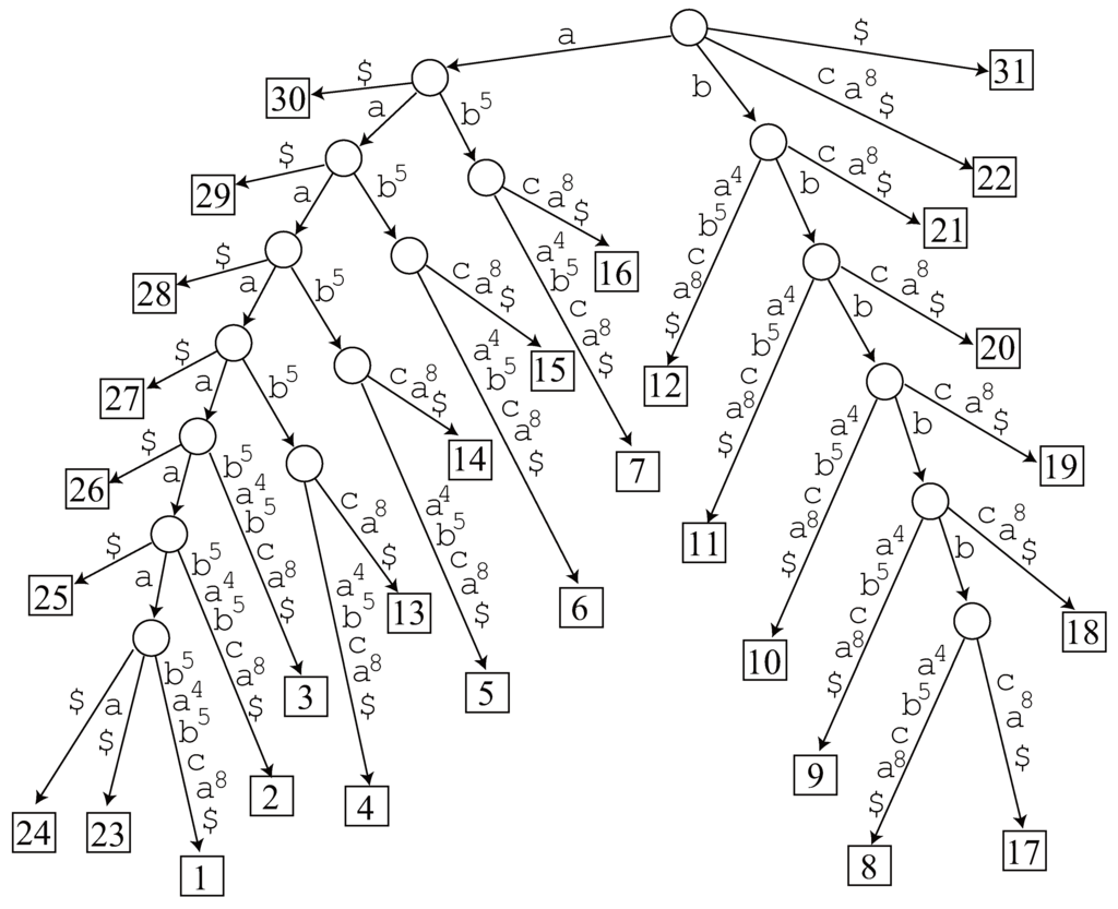
Figure 8.
with .
Now see Figure 9 which illustrates a generalized sparse suffix tree for
To find , we check the nodes in the list as follows.
- Length 8. The generalized suffix tree has no node representing , and hence it is not an LRF.
- Length 7. Since node exists in the generalized suffix tree, we traverse its subtree and find 2 occurrences 23 and 24 in . However, it is not an LRF of . The other candidate does not have a corresponding node in the tree, so it is not an LRF, either.
- Length 6. Node exists in the generalized suffix tree and we find 3 occurrences 23, 24 and 25 in by traversing the tree, but it is not an LRF. The tree has no node corresponding to , hence it is not an LRF.
- Length 5. Node exists in the generalized suffix tree and we find 4 occurrences 23, 24, 25 and 26 in by traversing the tree, but it is not an LRF. There is no node in the tree corresponding to .
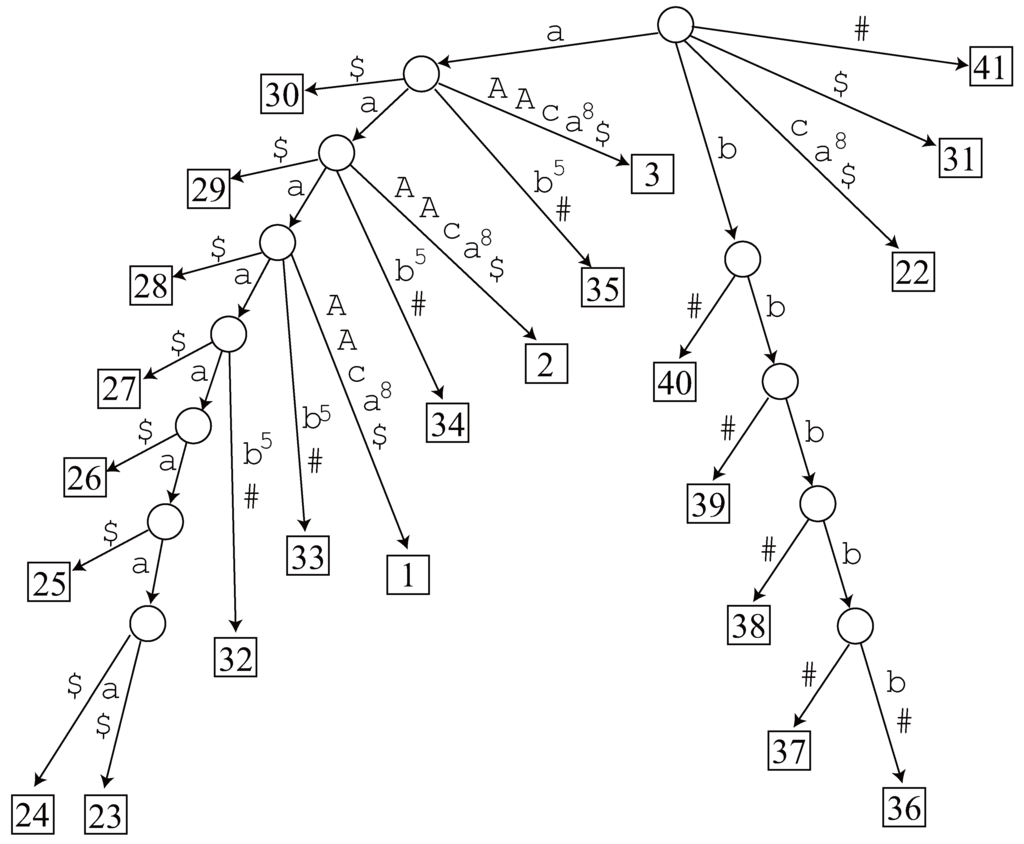
Figure 9.
Generalized sparse suffix tree of .
- Length 4. Node exists in the generalized suffix tree and we find 5 occurrences 23, 24, 25, 26 and 27. Now 23 and 27 are non-overlapping occurrences of , and hence it is an LRF of .
Focus on the above operations where we examined factors of lengths from 7 to 5. The total time cost to find the occurrences for the LRF-candidates of these lengths is proportional to 2 + 3 + 4, but none of them is an LRF of in the end.
In general, for any input string of the form
the time cost of the Lanctot algorithm for finding is proportional to
Since , the Lanctot algorithm takes time.
In his PhD thesis [33], Lanctot modified the algorithm so that all the occurrences of each candidate factor in w are stored in each element of the bin-sorted list (Section 3.1.3, page 55, line 1). However, this clearly requires space. Note that using a suffix array cannot immediately solve this, since the lexicographical ordering of the suffixes can change due to substitution of LRFs, and no efficient methods to edit suffix arrays for such a case are known.
On the contrary, as shown in Section 3, each node v of our data structure stores an ordered triple , and our algorithm properly maintains this information when the tree is updated. Using this triple, we can check in amortized constant time whether or not each node in the bin-sorted list is an LRF. Hence the total time cost remains .
© 2009 by the authors; licensee Molecular Diversity Preservation International, Basel, Switzerland. This article is an open access article distributed under the terms and conditions of the Creative Commons Attribution license (http://creativecommons.org/licenses/by/3.0/).