Radial Basis Function Cascade Correlation Networks

Abstract

A cascade correlation learning architecture has been devised for the first time for radial basis function processing units. The proposed algorithm was evaluated with two synthetic data sets and two chemical data sets by comparison with six other standard classifiers. The ability to detect a novel class and an imbalanced class were demonstrated with synthetic data.  In the chemical data sets, the growth regions of Italian olive oils were identified by their fatty acid profiles; mass spectra of polychlorobiphenyl compounds were classified by chlorine number. The prediction results by bootstrap Latin partition indicate that the proposed neural network is useful for pattern recognition.

1. Introduction

Artificial neural networks (ANNs) are widely used pattern recognition tools in chemometrics. The most commonly used neural network for chemists is the back-propagation neural network (BNN). The BNN is a feed forward neural network, usually trained by error back-propagation [1, 2]. BNNs have been applied to a broad range of chemical applications. Recent analytical applications of BNNs in fields such as differential mobility spectrometry [3] and near infrared spectroscopy [4] have been reported in the literature.

BNNs have been proven a useful type of ANNs in chemometrics. However, BNNs converge slowly during training especially when the network contains many hidden neurons. This slow and chaotic convergence is partially caused by the simultaneous adjustments of weights of all hidden neurons during the training of BNNs, which is referred to as the “moving target problem”. To avoid this problem, a network architecture named cascade correlation network (CCN) was proposed by Fahlman and Lebiere [5]. A CCN begins its training with a minimal network, which only has an input layer and an output layer. During training, the CCN determines its topology by adding and training one hidden neuron at a time, resulting in a multilayer structure. In this training strategy, the moving target problem is avoided because only weights of single hidden neuron in the network are allowed to change at any time. CCNs have been applied to the prediction of the protein secondary structure [6] and estimation of various ion concentrations in river water for water quality monitoring [7].

A temperature constrained cascade correlation network (TCCCN) [8], which combines the advantages of cascade correlation and computational temperature constraints was devised to provide reproducible models. By modifying the sigmoid transfer function, a temperature term is added to constrain the length of the weight vector in the hidden transfer function. The temperature is adjusted so that the magnitude of the first derivative of the covariance between the output and the residual error is maximized. As a result, fast training can be achieved because of the large weight gradient. TCCCNs have been successfully applied to many areas in analytical chemistry, such as identification of toxic industrial chemicals by their ion mobility spectra [9], classification of official and unofficial rhubarb samples based on their infrared reflectance spectrometry [10], and prediction of substructure and toxicity of pesticides from low-resolution mass spectra [11], etc.

Besides BNNs and CCNs, the radial basis function network (RBFN) is another important type of neural network. A RBFN is a three-layered feed forward network, which applies a radial basis function (RBF) as its hidden layer transfer function. The most commonly applied RBF is the Gaussian function. The determination of the number, centroids and radii of hidden units of RBFN can be achieved by different ways, such as random generation, clustering, and genetic algorithms. The RBFN can also be trained by back-propagation. Wan and Harrington developed a type of RBFN that is a self-configuring radial basis function network (SCRBFN) [12]. In a SCRBFN, a linear averaging (LA) clustering algorithm is applied to determine the parameters of the hidden units. Class memberships of the training objects are used during clustering in the LA algorithm.

Recently, many novel supervised learning methods have gained increasing popularity, such as the support vector machine (SVM) and Random Forest (RF). The SVM was introduced by Vapnik [13]. The SVM first maps the training data into high dimension feature space by using kernel functions. An optimal linear decision hyperplane is determined by maximizing the margin between the objects of two classes. The RF method was developed by Breiman [14]. It is derived from the decision trees algorithm. During the RF training, many decision trees were trained by the ensemble learning techniques. The classification result is then calculated by voting from all the trees built.

A radial basis function cascade correlation network (RBFCCN) that combines the advantages of CCNs and RBFNs was devised in the present work. The RBFCCN benefits from the RBF as the hidden transfer function instead of the commonly used sigmoid logistic function. The RBFCCN also has a cascade-correlation structure. The network performance was tested using both synthetic and actual chemical data sets. The partial least squares-discriminant analysis (PLS-DA) was also tested as the standard reference method. The theory of the PLS-DA can be found in the literature [15, 16]. Comparisons were made with the BNN, RBFN, SCRBFN, PLS-DA, SVM, and RF method. Two synthetic data sets, which are detection of a novel class data set and imbalanced data set, and two chemical data sets, which are Italian olive oil data set and polychlorobiphenyl (PCB) data set were evaluated. The bootstrap Latin partitions (BLPs) [17] validation method was used in this study.

2. Theory

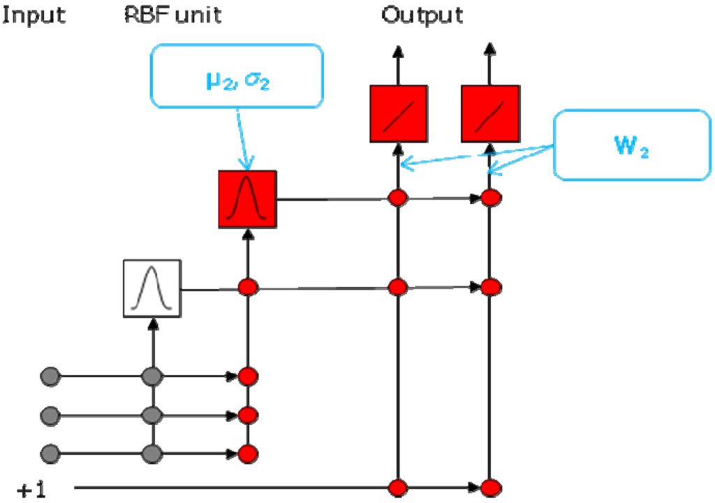
The network architectures of a RBFN and a RBFCCN are given in Figure 1 and Figure 2, respectively. By applying the cascade correlation algorithm, the RBFCCN has a different network topology compared with conventional RBFNs. In RBFCCNs, the transfer function applied in the hidden neuron is the Gaussian function. Unlike a RBFN that usually has only one hidden layer, the RBFCCN has a multi-layered structure. Each hidden layer contains only one neuron. In RBFCCNs, the kth hidden neuron is connected with k + l - 1 inputs, where l denotes the number of input neurons. The output of the ith object from the kth hidden neuron o_ik is given by:

$$o_{ik}=g_k\left({\text{x}}_{ik}\right)=\exp \left[-{\displaystyle \sum _{p=1}^{k+l-1}{\left(x_{ikp}-{\text{μ}}_{kp}\right)}^2/\left(2{\sigma }_k^2\right)}\right]$$

(1)

for which g_k is the notation of the Gaussian function; x_ik is the input vector; x_ikp is the corresponding pth element of x_ik. The µ_kp term denotes the pth element of centroid µ_k, and σ_k denotes the kth radius. The o_ik term will depend on two factors: the Euclidean distance between the sample and the centroid and the radius. In the cascade-correlation training architecture, the hidden units are added and trained sequentially during training.

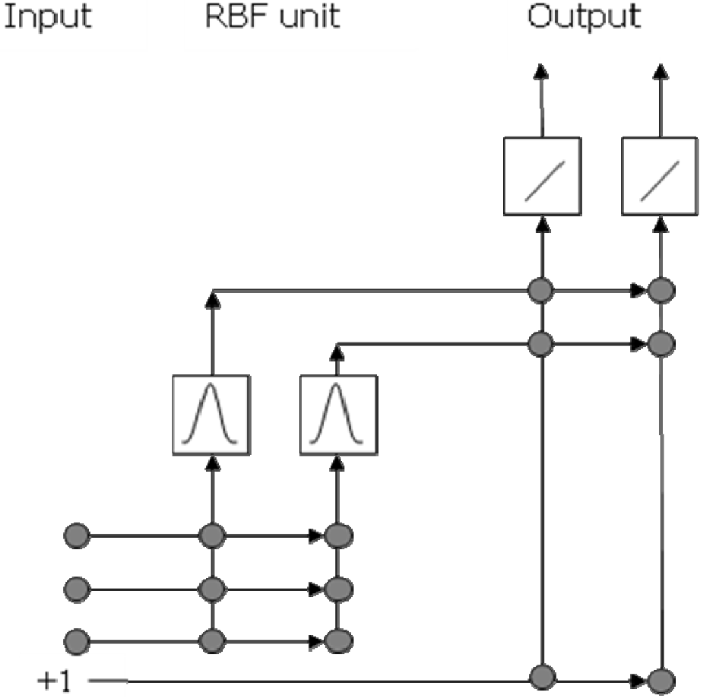
Figure 1. Network architecture of a RBFN. This network has three input neurons, two hidden neurons, and two output neurons.

Figure 1. Network architecture of a RBFN. This network has three input neurons, two hidden neurons, and two output neurons.

Figure 2. Network architecture of a RBFCCN. This network has three input neurons, two hidden neurons, and two output neurons.

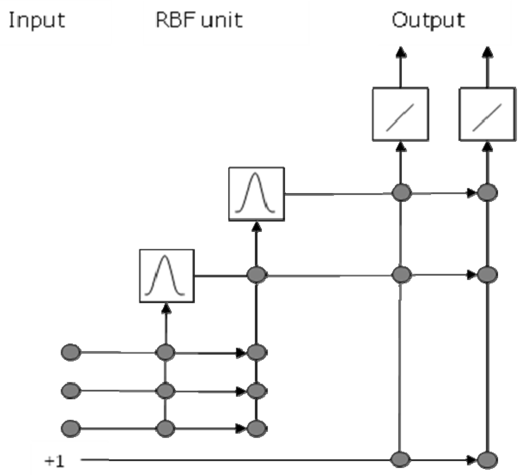
Figure 2. Network architecture of a RBFCCN. This network has three input neurons, two hidden neurons, and two output neurons.

The training process of a RBFCCN includes the following steps:

• Initialize the network.
• Add a hidden neuron to the network. Initialize this hidden neuron by setting initial values of µ_k and σ_k of the Gaussian function.
• Train the hidden neuron. Determine the values of µ_k and σ_k.
• Train the weights W_k in the output layer.
• Repeat step 2 to step 4 until a given error threshold is achieved or a given number of hidden units were added.

2.1. Initialize the RBFCCN

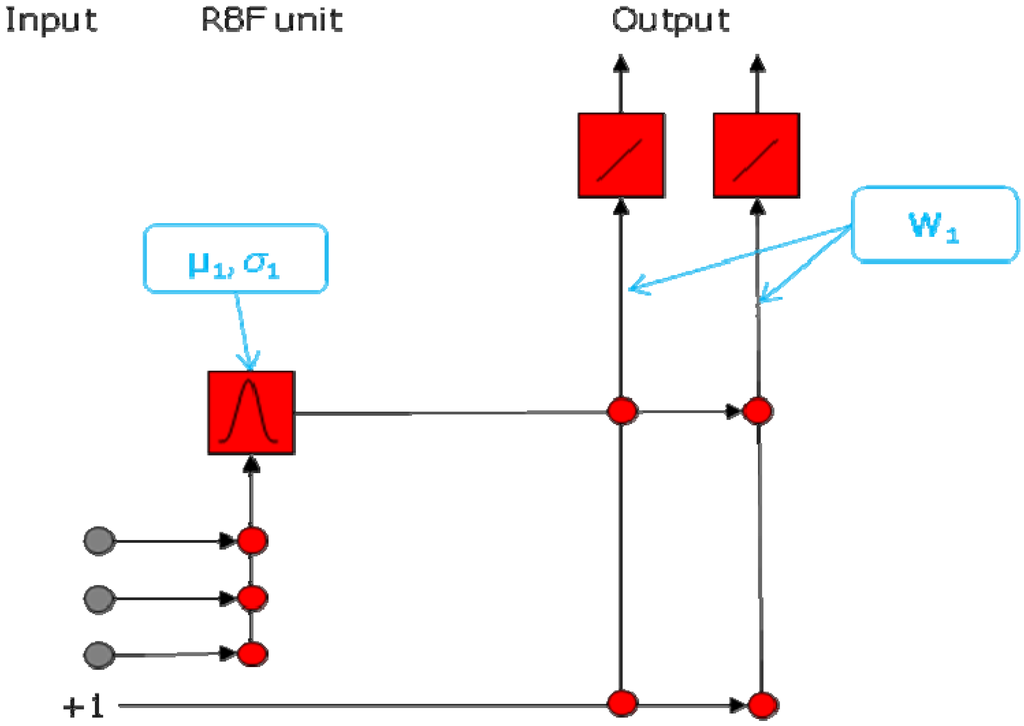
The RBFCCN initialization is given in Figure 3. RBFCCN begins its training with a minimal network, which only has an input layer and an output layer. The number of input neurons l is equal to the number of variables of the data set. The number of output neurons n is equal to the number of classes in the training set. The neurons in the output layer are linear.

In this work, binary coding is used to determine the training target value. Each class has a corresponding binary sequence of unity or zero in which an element of unity indicates the identity of the object’s class membership. For example, the output vector for objects belonging to the second class in a training set of four classes will be encoded (0, 1, 0, 0) as the training target value, i.e., the desired output vector of the trained network model is (0, 1, 0, 0).

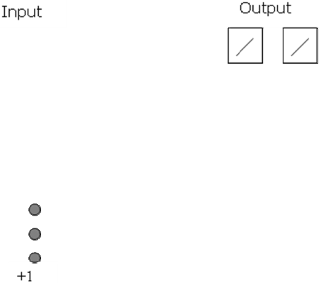
Figure 3. Network initialization of a RBFCCN. This network has three input neurons and two output neurons.

Figure 3. Network initialization of a RBFCCN. This network has three input neurons and two output neurons.

2.2. Add and initialize a hidden neuron

Figure 4 and Figure 5 demonstrate adding the first and second hidden neurons to the RBFCCN, respectively. Unlike the CCN that adds and trains a pool of candidate neurons, the RBFCCN adds and trains only one hidden neuron at a time because the initialization method applied in the RBFCCN is deterministic.

The trained neuron of the RBFCCN is unique. Once the kth hidden neuron is added to the RBFCCN, the centroid µ_k is initialized with the mean vector of the target objects, and the initial radius σ_k is given by the mean of the standard deviations of the target objects. The target objects of the kth hidden neuron are training objects from t_kth training class. When k ≤ n, for which n denotes the number of training classes, t_k = k. When k > n, t_k is the class that contains the maximum total residual error among all training classes. According to the central limit theorem, it is assumed that all the objects from the same class tend to be normally distributed in the input space. The Gaussian function will represent a class of objects in the input space in this case. The initial hidden units represent clusters of the training data just as LA clustering does. This initialization method has advantages over the random initialization method in that the value is fixed so it will converge faster.

Figure 4. Adding first hidden neurons into a RBFCCN. This network has three input neurons, one hidden neuron and two output neurons. The neurons and connections being trained are marked in red. µ₁, σ₁ and W₁ are parameters to be trained.

Figure 4. Adding first hidden neurons into a RBFCCN. This network has three input neurons, one hidden neuron and two output neurons. The neurons and connections being trained are marked in red. µ₁, σ₁ and W₁ are parameters to be trained.

Figure 5. Adding second hidden neurons into a RBFCCN. This network has three input neurons, two hidden neurons and two output neurons. The neurons and connections being trained are marked in red. µ₂, σ₂ and W₂ are parameters to be trained.

Figure 5. Adding second hidden neurons into a RBFCCN. This network has three input neurons, two hidden neurons and two output neurons. The neurons and connections being trained are marked in red. µ₂, σ₂ and W₂ are parameters to be trained.

2.3. Train the hidden neuron

The training strategy of the hidden neuron is adopted from that of the CCN. After initialization, the centroids µ_k and radii σ_k are trained by maximizing the covariance between the output and the target value of a hidden unit by appropriate optimization algorithms. The covariance C_k from the kth hidden unit is given by:

$$C_k={\displaystyle \sum _{i=1}^m\left(o_{ik}-{\overline{o}}_k\right)}{y}_{ik}$$

(2)

for which o_ik is the output of the ith observation and the kth hidden neuron; y_ik is the corresponding target value; m is the total number of training objects. Once a hidden neuron is trained, the centroid and radius of it will remain unchanged for the rest of the network training process.

Instead of using all training objects as target values, only objects in the t_kth training class are selected as the target value for the training of the hidden neurons, for which t_k is the target class membership used in initializing kth hidden neuron. As a result, the target value y_ik of the ith object and the kth hidden neuron is given by:

$$y_{ik}=\{\begin{array}{l}1\left(c_i=t_k\right)\\ 0\left(c_i\ne t_k\right)\end{array}$$

(3)

where c_i is the class membership of the ith training object.

2.4. Train the weights in the output layer

The weights in the output layer are recalculated and stored after each hidden neuron is added and trained. As the case in TCCCNs, the input units do not connect to the output units directly. The predicted value ${\widehat{Y}}_k$ of the network with kth hidden neurons is calculated by the product of the output matrix O_k and the weight matrix W_k, which is given by

$${\widehat{\text{Y}}}_k={{\rm O}}_k{\text{W}}_k$$

(4)

for which O_k is the output matrix for the hidden neurons. The matrix is augmented with a column of unity, which allows a bias value to be calculated. Therefore, the output matrix O_k has m rows and k + 1 columns, for which m denotes the total number of training objects. The weight matrix W_k stores the weight vector of the output layer. The W_k matrix has k + 1 rows and n columns, for which n denotes the number of classes of the training object. Singular value decomposition (SVD) is applied to determine the values of the weight vectors. The SVD of O_k is given by:

$${{\rm O}}_k={\text{U}}_k{\text{S}}_k{{\text{V}}_k}^{{\rm T}}$$

(5)

in which U_k and V_k are eigenvectors that respectively span the column and row spaces for the O_j matrix, and S_k is the singular value matrix. By using SVD, the pseudoinverse of O_k can be computed with ${\text{V}}_k{{\text{S}}_k}^{\text{-1}}{{\text{U}}_k}^{{\rm T}}$. According to Eq. 4, W_k is given by:

$${\text{W}}_k=\text{Y}{\text{V}}_k{{\text{S}}_k}^{\text{-1}}{{\text{U}}_k}^{{\rm T}}$$

(6)

for which Y is the target value matrix of the whole training set.

2.5. Evaluate the stopping condition of RBFCCN

The RBFCCN can be trained until a given number of hidden units were added and trained, or a given error threshold is achieved. The relative root mean square error of calibration (RRMSEC) was used in this work. The RRMSEC is given by:

$$RRMSEC=\sqrt{\frac{{\displaystyle {\sum }_{i=1}^m{\displaystyle {\sum }_{j=1}^n{\left({\widehat{y}}_{ij}-y_{ij}\right)}^2}}}{{\displaystyle {\sum }_{i=1}^m{\displaystyle {\sum }_{j=1}^n{\left(y_{ij}-{\overline{y}}_j\right)}^2}}}}$$

(7)

for which m is the total number of training objects, n is the number of classes, y_ij is the target value for the ith object and class j, ${\widehat{y}}_{ij}$ is the network model output for object i and class j, and ${\overline{y}}_j$ is the average target value for class j. To have a relative metric, the standard error of calibration is corrected by the standard deviation. By applying the RRMSEC thresholds, the experimental results only depend on different network topologies. Different training algorithms such as QuickProp, Rprop, and Bayesian approach affect the convergence time and achieve equivalent classification accuracies for the training sets.

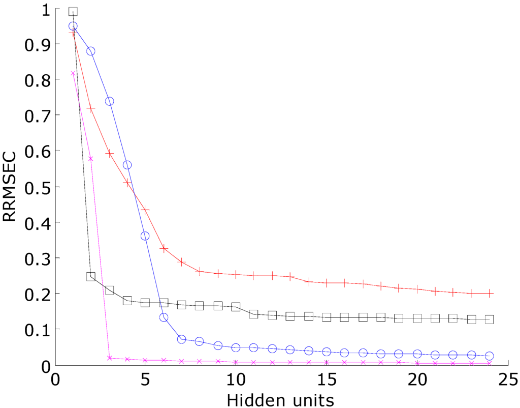
Figure 6. The RRMSEC with respect to hidden unit number trained by the RBFCCN using one training data set from the bootstrapped Latin partition. Magenta line with cross sign marker: novel class data set; black line with box marker: imbalanced data set; red line with plus sign marker: Italian olive oil data set; blue line with circle marker: PCB data set.

Figure 6. The RRMSEC with respect to hidden unit number trained by the RBFCCN using one training data set from the bootstrapped Latin partition. Magenta line with cross sign marker: novel class data set; black line with box marker: imbalanced data set; red line with plus sign marker: Italian olive oil data set; blue line with circle marker: PCB data set.

Figure 6 shows the RRMSEC with respect to hidden unit number trained by the RBFCCN. The RRMSEC thresholds were determined by training a RBFCCN model using one training data set from the bootstrapped Latin partition until the RRMSEC is not significantly improved. Once the RRMSEC threshold is determined, it is applied to train all the other neural networks. Of course, this method is biased in favor of the RBFCCN but it is required so that all the other reference classifiers have the same performance. However, the primary goal of this research is to compare the prediction accuracies and the ability of the different classifiers to generalize when trained to similar target values of classification accuracies. Because the training methods of the diverse set of classifiers that are used for comparison are inherently different, it is important to address that the RRMSEC threshold is only applied to train the network models to the same classification accuracy for the training sets.

2.6. Identify the class membership

The class membership of an object is determined by its corresponding output vector from the network model using the following strategies. When all the outputs are below a given threshold, the object is labeled as unknown. The threshold is 0.5 in this study. Otherwise, the class is determined by the winner-take-all method, in which the unknown is classified by the index of the maximum element in the output vector. The SVM and RF have their own novel class evaluation procedure, which is not discussed in this paper. Therefore, the SVM and RF methods were excluded from the novel class evaluation.

2.7. Advantages of RBFCCN

The RBFCCN offers several advantages. The cascade-correlation architecture has the ability of incremental learning. The term incremental learning means that the network builds its topology during training by adding and training one hidden unit at a time. The first advantage is that the incremental learning ability avoids the moving target problem in the BNN and the network converges rapidly. Second, by training to a threshold of residual error, the cascade-correlation architecture does not require to determine the amount of hidden units in the network before training. Third, multiple networks can be obtained by training only once. These trained networks are networks with hidden units ranging from one to the total number of hidden units added to the cascade-correlation network. Fourth, by using RBF transfer functions, RBFCCNs are suitable for performing novel class evaluation, i.e., the ability to identify unknown data or outliers in a data set.

3. Experimental section

3.1. General information

All calculations were performed on an AMD Athlon XP 3000+ personal computer running Microsoft Windows XP SP3 operating system. The programs were in-house scripts written in MATLAB version 7.5, except for the analysis of variance (ANOVA), SVM, and RF. ANOVA was performed in Microsoft Excel version 12.0. The SVM calculations were performed by the LIBSVM software version 2.89 with MATLAB interface [18]. The RF program was obtained from reference [19]. The training of RBFCCN was implemented through fminbnd and fminunc functions by their default parameters from the optimization toolbox version 3.1.2 of MATLAB. The fminunc function uses the Broyden-Fletcher-Goldfarb-Shanno (BFGS) quasi-Newton method with a cubic line search procedure. The fminbnd function is based on golden section search and parabolic interpolation algorithm. In the RBFCCN, RBFN, and SCRBFN, the weights of the output neurons were updated by the SVD algorithm. The SVD algorithm was implemented by the MATLAB function pinv. All ANNs and PLS-DA applied binary coding for determine the classes from the outputs.

Instead of training neural networks to achieve the minimum error of an external validation set, all the neural networks (the BNNs, SCRBFNs, RBFNs, and RBFCCNs) compared in this work were trained to a given RRMSEC in each data set. All the neural networks and PLS-DA applied the binary coding method to set the training target value, and the method to identify the class membership stated above. The BNNs used in this work consists of three layers: one input layer, one hidden layer and one output layer. The sigmoid neuron was used in the hidden layer, and the output layer was linear. The two-stage training method of RBFN was applied. The centroids and radii of RBFN were initialized by the K-means clustering, and optimized by back-propagation. The centroid of the kth hidden neuron µ_k was initialized by the mean of the objects in the kth cluster, and the radius of the kth hidden neuron σ_k was initialized by:

$${\sigma }_k=\left({\displaystyle \sum _{q=1}^3{\Vert {\text{μ}}_k-{\text{μ}}_q\Vert }^2}\right)/\sqrt{3}$$

(8)

for which µ_q is the three nearest neighbors of µ_k. The details of this method are described in reference [20]. In the SCRBFNs, the parameter λ in the linear averaging clustering algorithm was adjusted gradually to achieve the RRMSEC.

For the RBFN model, the number of hidden neurons h equals to the number of training classes. For the BNN model, h is empirically proposed by:

$$h=\{\begin{array}{l}n(l\le n)\\ \text{round}(l+n/2)(l>n)\end{array}$$

(9)

for which l denotes the number of variables of the data set, n denotes the number of classes of the training object, and round denotes round to the closest integer. Because two synthetic data sets were relatively simple in data size that have less variables and classes, h was fixed without further evaluations. To demonstrate the numbers of hidden neurons was appropriate, independent tests were performed by evaluating BNNs on two chemical data sets with 0.5h and 2h hidden neurons so that the network performances can be observed by significantly decreasing or increasing the hidden layer size. Table 1 gives the average prediction accuracies of the BNN models of Italian olive oil and the training set of the PCB data set. For the Italian olive oil data set, the BNN models with 7 and 14 hidden neurons did not significantly differ with respect to prediction accuracy. The BNN models with four hidden neurons had too few hidden units to model the data sufficiently. For the PCB dataset, the effect of the three different numbers of hidden neurons on the prediction results was not significant. The BNNs with extra hidden neurons will not overfit the data if trained to the same RRMSEC. As a result, the heuristic equation of h was appropriate.

Table 1. Average prediction accuracies of the BNN models with 95% confidence intervals of Italian olive oil and the training set of the PCB data set. The BNN was trained by different number of hidden neurons with 30 BLPs.

Data set	Number of hidden neurons	Prediction accuracy
Olive oil	7	95.5 ± 0.3
	14	95.9 ± 0.4
	4	87.7 ± 0.2
PCB	13	99.9 ± 0.1
	26	99.9 ± 0.1
	7	99.9 ± 0.1

Table 1. Average prediction accuracies of the BNN models with 95% confidence intervals of Italian olive oil and the training set of the PCB data set. The BNN was trained by different number of hidden neurons with 30 BLPs.

Data set	Number of hidden neurons	Prediction accuracy
Olive oil	7	95.5 ± 0.3
	14	95.9 ± 0.4
	4	87.7 ± 0.2
PCB	13	99.9 ± 0.1
	26	99.9 ± 0.1
	7	99.9 ± 0.1

To determine the learning rates and momenta of the BNNs and RBFNs, these networks were trained by three different sets of learning rates and momenta with BLPs. The number of bootstraps was 30 and the number of partitions was two. Table 2 gives the prediction results by the Italian olive oil data set and the training set of the PCB data set. The training parameters of the back-propagation networks did not significantly affect the comparison of the modeling methods. These sets of learning parameters were also trained by the two synthetic data sets and same results were obtained. For each data set, there was no statistical difference of the BNN and RBFN prediction results at a 95% confidence interval by two-way ANOVA with interaction. Therefore, the learning rates and momenta were fixed respectively at 0.001 and 0.5 for all further evaluations.

Table 2. Average prediction accuracies of the BNN and RBFN models with 95% confidence intervals of Italian olive oil and the PCB data sets. The BNN and RBFN were trained by three different sets of learning rates and momenta with 30 BLPs.

Data set	Learning rate	Momentum	BNN	RBFN
Olive oil	0.001	0.5	95.5 ± 0.3	92.0 ± 0.7
	1 × 10-4	0.5	95.4 ± 0.3	91.9 ± 0.7
	0.001	0	95.6 ± 0.3	91.5 ± 0.6
PCB	0.001	0.5	99.9 ± 0.1	92.4 ± 5.5
	1 × 10-4	0.5	99.5 ± 0.2	90.8 ± 6.3
	0.001	0	99.9 ± 0.1	94.1 ± 4.8

Table 2. Average prediction accuracies of the BNN and RBFN models with 95% confidence intervals of Italian olive oil and the PCB data sets. The BNN and RBFN were trained by three different sets of learning rates and momenta with 30 BLPs.

Data set	Learning rate	Momentum	BNN	RBFN
Olive oil	0.001	0.5	95.5 ± 0.3	92.0 ± 0.7
	1 × 10-4	0.5	95.4 ± 0.3	91.9 ± 0.7
	0.001	0	95.6 ± 0.3	91.5 ± 0.6
PCB	0.001	0.5	99.9 ± 0.1	92.4 ± 5.5
	1 × 10-4	0.5	99.5 ± 0.2	90.8 ± 6.3
	0.001	0	99.9 ± 0.1	94.1 ± 4.8

The PLS-DA was implemented by the non-linear iterative partial least squares (NIPALS) algorithm. The number of latent variables was determined by minimizing the root mean squared prediction error in each test. As a result, the PLS-DA was a biased reference method. The numbers of latent variables in the PLS-DA models may vary between runs.

All the SVMs used the Gaussian RBF as their kernel functions. Two SVM parameters: the cost c and the RBF kernel parameter γ must be adjusted before each prediction. The grid search of parameter pairs (c, γ), in which c = 2ⁱ, i = -2, -1, 0, …, 20; γ = 2^j, j = -10, -9, -8, …, 10, was performed to determine their value by achieving the best training accuracies. The defaults of the remaining parameters were used. Because the result of the RF algorithm is not sensitive to the parameter selected, 1,000 trees with the default setting of the number of variables to split on at each node is used in all evaluations.

The BLPs generates precision measures of the classification. Bootstrapping is a method that re-samples the data. Latin partition is a modified cross-validation method, in which the class distributions are maintained at constant proportions among the entire data set and the randomized splits into training and prediction sets. After the data set was partitioned during each bootstrap, it was evaluated by all the modeling methods in the study. Because bootstrapping runs the evaluation repeatedly, the confidence interval of the prediction errors can also be obtained. The number of bootstraps was 30 and the number of partitions was two for evaluating all the data sets in this study. The results are reported as prediction accuracy, which is the percentage of correctly predicted objects. To determine the classification ability of RBFCCN, four data sets were tested, including the novel class data set, imbalanced data set, Italian olive oil data set, and the PCB data set. The numbers of variables, objects, and classes of data sets are given in Table 3. The modeling parameters of the ANNs, PLS-DA, SVM, and RF method are given in Table 4. Similar to the latent variables used in the PLS-DA models, the numbers of hidden neurons used to train SCRBFN and RBFCCN models may vary between different runs. Therefore, only typical latent variables and numbers of hidden neurons are reported.

Table 3. The numbers of variables, objects, and classes of the data sets evaluated.

	Novel class		Imbalanced		Olive oil	PCB
	Training	Test	Training	Test	BLP validation	BLP validation	External validation
Variables	2	2	2	2	8	18a	18a
Objects	400	100	610	10	478	131	154
Classes	4	1	3	1	6	7	8b

^aThis number is the number of variables after the modulo method of preprocessing.^bThe PCB congeners that contain 0, 1, 9 and 10 chlorine atoms were considered as one class.

Table 3. The numbers of variables, objects, and classes of the data sets evaluated.

	Novel class		Imbalanced		Olive oil	PCB
	Training	Test	Training	Test	BLP validation	BLP validation	External validation
Variables	2	2	2	2	8	18a	18a
Objects	400	100	610	10	478	131	154
Classes	4	1	3	1	6	7	8b

^aThis number is the number of variables after the modulo method of preprocessing.^bThe PCB congeners that contain 0, 1, 9 and 10 chlorine atoms were considered as one class.

Table 4. The modeling parameters of the ANNs, PLS-DA, SVM, and RF method. Hidden units are the number of hidden units in the trained network model. Latent variables are the number of latent variables used in the PLS-DA models. The RBF kernel parameter is denoted by γ in the SVM method. Mtry is the number of variables to split on at each node in the RF method.

	Modeling parameters	Novel class	Imbalanced	Olive oil	PCB
	RRMSEC threshold	0.02	0.2	0.4	0.1
BNN	Learning rate	0.001	0.001	0.001	0.001
	Momentum	0.5	0.5	0.5	0.5
	Hidden units	4	3	7	13
RBFN	Learning rate	0.001	0.001	0.001	0.001
	Momentum	0.5	0.5	0.5	0.5
	Hidden units	4	3	6	7
SCRBFN	Hidden units	-	17	~6	~20-30
RBFCCN	Hidden units	4	3	~6	~8
PLS-DA	Latent variables	-	2	~8	~16-18
SVM	Cost	-	210	210	213
	γ	-	2-1	1	2-5
RF	Number of trees	-	1000	1000	1000
	Mtry	-	1	2	4

Table 4. The modeling parameters of the ANNs, PLS-DA, SVM, and RF method. Hidden units are the number of hidden units in the trained network model. Latent variables are the number of latent variables used in the PLS-DA models. The RBF kernel parameter is denoted by γ in the SVM method. Mtry is the number of variables to split on at each node in the RF method.

	Modeling parameters	Novel class	Imbalanced	Olive oil	PCB
	RRMSEC threshold	0.02	0.2	0.4	0.1
BNN	Learning rate	0.001	0.001	0.001	0.001
	Momentum	0.5	0.5	0.5	0.5
	Hidden units	4	3	7	13
RBFN	Learning rate	0.001	0.001	0.001	0.001
	Momentum	0.5	0.5	0.5	0.5
	Hidden units	4	3	6	7
SCRBFN	Hidden units	-	17	~6	~20-30
RBFCCN	Hidden units	4	3	~6	~8
PLS-DA	Latent variables	-	2	~8	~16-18
SVM	Cost	-	210	210	213
	γ	-	2-1	1	2-5
RF	Number of trees	-	1000	1000	1000
	Mtry	-	1	2	4

3.2. Detection of a novel class using a synthetic data set

This synthetic data set was designed to test the BNN, RBFN, and RBFCCN abilities to respond to a novel class during prediction. The training set comprised two variables and four classes. Each training class and the test objects had 100 objects. Each class was normally distributed with means of (0.0, 0.0), (40.0, 0.0), (0.0, 40.0), and (40.0, 40.0), respectively, with a standard deviation of 1.5. The test objects were distributed about a mean of (20.0, 20.0) with a standard deviation of 1.5. Both networks were trained repeatedly 30 times on this data set to obtain statistically reliable results.

3.3. Synthetic imbalanced data set

An imbalanced data set is a data set that the numbers of objects are not equal in each class. This data set was designed to compare the performances when the data set is highly imbalanced. This data set had two variables. The training set comprised three normally distributed classes. Two classes were majority classes, which have 300 objects respectively distributed with means of (3.0, 0.0), (-3.0, 0.0) and with standard deviations of unity. The other training class was the minority class that has only 10 objects distributed about a mean of (0.0, 0.0) with a standard deviation of 0.1. The test class had the same distribution with the minority training class. The ANNs were trained to the RRMSEC thresholds of 0.2. The network performances were evaluated by predicting the minority class in the training set. All modeling methods were reconstructed 30 times to obtain statistically reliable results.

3.4. Italian olive oil data set

Italian olive oil data were obtained from references [21, 22]. This data set is a well-studied standard reference data set. Different source regions of Italian olive oil were classified by the profile of eight different fatty acids. To minimize the effect of class imbalance and obtain fair comparison results, objects from smaller classes that have less than 50 objects were removed from the evaluation data. The number of classes was six. Each variable in the training sets was scaled between 0 and 1. The variables of the test sets in each Latin partition were scaled using the range acquired from the training set to obtain unbiased results. The training RRMSEC thresholds were 0.4.

3.5. PCB data set

In the PCB data set, PCB congeners with different numbers of chlorine atoms were classified by their electron ionization mass spectra. The data set was used previously [8, 12]. The mass spectra were obtained from reference [23]. These spectra were split into the training set and the external validation set. The PCB congeners in the training set contained 2 to 8 chlorine atoms. Most of the PCB congeners have duplicate spectra with variable quality. Among these duplicate spectra, the one with the lowest record number was selected as training spectra, because it was the spectrum of highest quality. The PCB congeners in the external validation set contained 0 to 10 chlorine atoms. The external validation set was built from the remaining duplicate spectra, PCB congeners that have less than 10 objects, and 27 non-PCB compounds. The congeners that contain 0, 1, 9 and 10 chlorine atoms were uniquely different from any of the training classes. The external validation set contained 45 unique spectra.

Each spectrum was centered by its mean and normalized to unit vector length. The spectra were transformed to a unit mass-to-charge ratio scale that ranged from 50 to 550 Th and any peaks outside this range were excluded. Because the raw data were underdetermined, i.e., there were more variables than objects, the dimensions of PCB data set were further reduced by using the modulo method of preprocessing [24, 25]. This compression method is especially effective for mass spectral data. Based on the previous study [8] by the principal component analysis (PCA), the divisor value of 18 was chosen. The compressed spectra were centered about their mean and normalized to unit vector length. The training RRMSEC thresholds were 0.1.

4. Results and Discussion

4.1. Detection of a novel class using a synthetic data set

The bivariate plot of the synthetic data set is given in Figure 7. The response surface of the BNN is given in Figure 8.

RBFN and RBFCCN networks have similar response surfaces that are given in Figure 9. For each sampling point, the maximum of the output neurons is plotted. Because of the different shapes and properties of the sigmoid function and the Gaussian function, these networks have unique response surfaces. The BNN model gave an open, sigmoidal shaped response surface that divides the output space into regions that correspond to the four classes. When the BNN model extrapolates outside the region defined by the data objects, the response can be larger than unity, which occurs when the output units are linear. Alternatively, the RBFCCN and RBFN had a Gaussian shaped response surface that has a finite span of the output space, which is closed and compact. The maximum response of RBFCCN is unity.

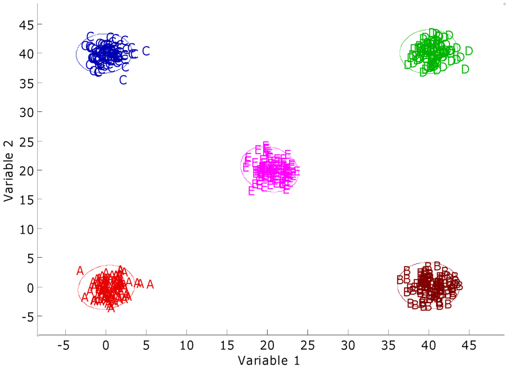
Figure 7. Two-variable plot of the synthetic novel class data set. A, B, C, and D denote the training sets, and E denotes the test set. The 95% confidence intervals were calculated around each training class.

Figure 7. Two-variable plot of the synthetic novel class data set. A, B, C, and D denote the training sets, and E denotes the test set. The 95% confidence intervals were calculated around each training class.

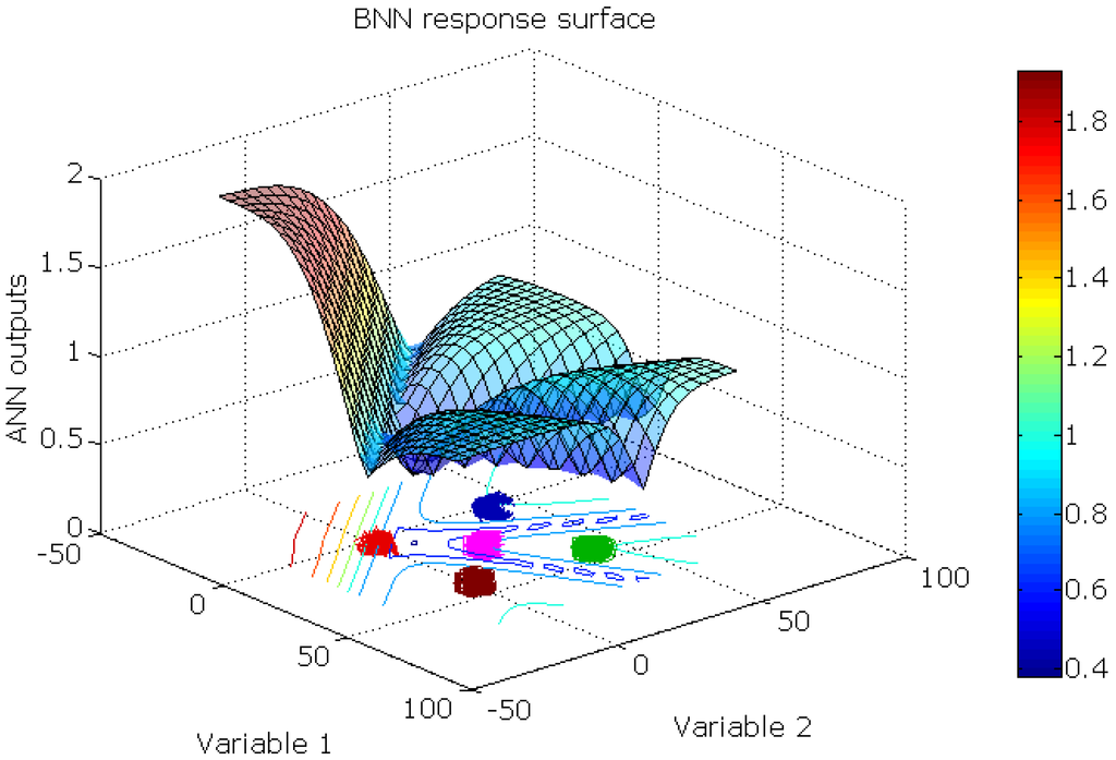
Figure 8. The BNN response surface of the synthetic novel class data set. For each sampling point, the maximum of the output neurons is plotted.

Figure 8. The BNN response surface of the synthetic novel class data set. For each sampling point, the maximum of the output neurons is plotted.

Figure 9. The RBFN and RBFCCN response surface of the synthetic novel class data set. For each sampling point, the maximum of the output neurons is plotted.

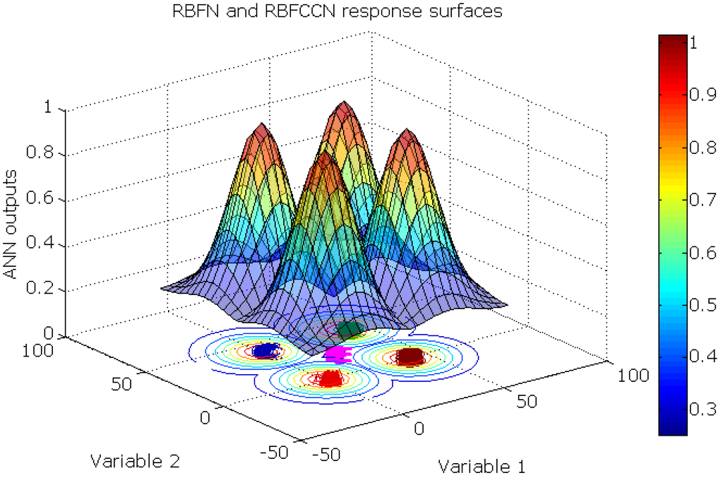
Figure 9. The RBFN and RBFCCN response surface of the synthetic novel class data set. For each sampling point, the maximum of the output neurons is plotted.

The test set was designed to be uniquely different from the data in the training set. The ideal prediction results of these test objects should be no excitation from any of the output neurons, i.e., the outputs are (0, 0, 0, 0).

Figure 10. Average prediction outputs from the test set. BNN, RBFCCN and RBFN models were obtained by training each network 30 times. The 95% confidence intervals are indicated as the thin lines around the BNN outputs. Different colors represent excitations from different output neurons.

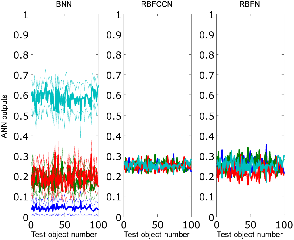
Figure 10. Average prediction outputs from the test set. BNN, RBFCCN and RBFN models were obtained by training each network 30 times. The 95% confidence intervals are indicated as the thin lines around the BNN outputs. Different colors represent excitations from different output neurons.

Figure 10 gives different outputs of the test set with respect to the different models. The outputs of RBFCCN and RBFN were the same for all repeats. The trained BNN models have different weights between different times of training. Because in most cases one output element was larger than 0.5, the BNN models misclassified most of the test objects as one of the training classes. The RBFCCN and RBFN models correctly identified all test objects as unknown. Compared to the RBFN models, the prediction results of RBFCCN models were closer to the ideal solution, because the outputs from the RBFN models spread more widely than the RBFCCN models.

4.2. Synthetic imbalanced data set

The bivariate plot of the synthetic imbalanced data set is given in Figure 11. It can be observed that objects in two majority classes have larger spans than the minority classes in the input space. The predictions of small classes by different ANNs are given in Table 5. The prediction results of the SCRBFN and RBFCCN models are better than the prediction results of the BNN and PLS-DA models. The RBFCCN, SVM, and RF methods have better predictions among all seven methods. The RBFN models have slightly worse prediction result than the three methods above. The trained models of the ANNs will have a relatively loose fit to the training set by setting the training error threshold to 0.2. The BNN and PLS-DA models trend to first model the majority classes in the prediction class. As a result, predictions of minority classes are poor.

Figure 11. Two-variable plot of the synthetic imbalanced data set. A (red), B, and C denote the training classes. D (green) denotes test class. The 95% confidence intervals were calculated around each training class.

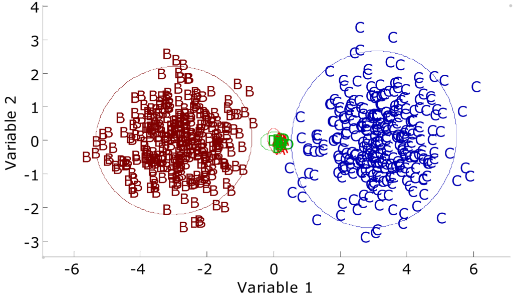
Figure 11. Two-variable plot of the synthetic imbalanced data set. A (red), B, and C denote the training classes. D (green) denotes test class. The 95% confidence intervals were calculated around each training class.

Table 5. Average numbers of correctly predicted objects with 95% confidence intervals from class D in an imbalanced data set by different models. All modeling methods were reconstructed 30 times.

	Total	BNN	SCRBFN	RBFN	RBFCCN	PLS-DA	SVM	RF
Correctly predicted	10	0	7	9.1 ± 0.1	10	0	10	10

Table 5. Average numbers of correctly predicted objects with 95% confidence intervals from class D in an imbalanced data set by different models. All modeling methods were reconstructed 30 times.

	Total	BNN	SCRBFN	RBFN	RBFCCN	PLS-DA	SVM	RF
Correctly predicted	10	0	7	9.1 ± 0.1	10	0	10	10

4.3. Italian olive oil data set

The principal component scores of the Italian olive oil data set are given in Figure 12. From this plot, it can be seen that objects in the same classes form clusters, but the confidence intervals are overlapped with each other. The prediction accuracies of different ANN models are given in Table 6. SVM and RF models have the highest prediction accuracy of 97.9%. The results calculated by the BNN and RBFCCN models are better than the results calculated by the SCRBFN and RBFN models. The PLS-DA models yield a lower average prediction accuracy of 89.8%. A two-way ANOVA with interaction at a significance level of 0.05 was performed to analyze the sources of variation and prediction accuracies. The results of ANOVA are given in Table 7. Different modeling methods, different source regions and the interaction between the classifiers show significant differences in prediction. The ANOVA results indicate that the methods evaluated have different performances. The SVM and RF perform best among the methods evaluated. The RBFCCN and BNN have statistically better performance in predicting this data set compared to PLS-DA, RBFN and SCRBFN.

Figure 12. A principal component score plot for the olive oil data set. Each axis is labeled with the percent total variance and the absolute eigenvalue. Each observation of the data set was scaled to [0, 1]. The 95% confidence intervals appear as an ellipse around each class. The sources regions are: (A) Calabria; (B) South Apulia; (C) Inland Sardinia; (D) East Liguria; (E) West Liguria; (F) Umbria.

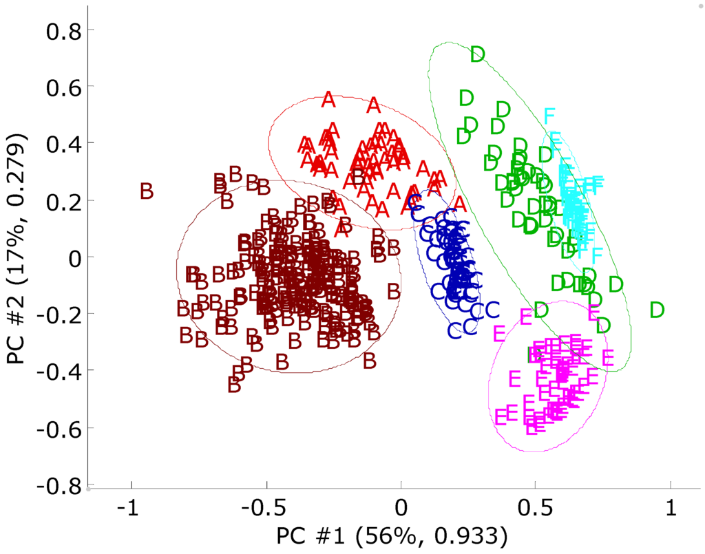
Figure 12. A principal component score plot for the olive oil data set. Each axis is labeled with the percent total variance and the absolute eigenvalue. Each observation of the data set was scaled to [0, 1]. The 95% confidence intervals appear as an ellipse around each class. The sources regions are: (A) Calabria; (B) South Apulia; (C) Inland Sardinia; (D) East Liguria; (E) West Liguria; (F) Umbria.

Table 6. Average numbers of correctly predicted objects with 95% confidence intervals of Italian olive oil data set by different modeling methods with 30 BLPs.

Source regions	Total	BNN	SCRBFN	RBFN	RBFCCN
Calabria	56	50.9 ± 0.6	50.3 ± 0.5	52.5 ± 0.6	52.7 ± 0.2
South Apulia	206	203.8 ± 0.5	199.5 ± 0.6	203.5 ± 0.4	200.1 ± 0.3
Inland Sardin	65	65	58.3 ± 0.3	63.4 ± 0.4	64.2 ± 0.2
East Liguria	50	38.0 ± 1.0	37.4 ± 0.7	24.4 ± 3.6	35.4 ± 0.7
West Liguria	50	48.2 ± 0.3	43.3 ± 0.5	47.6 ± 0.8	48.5 ± 0.3
Umbria	51	50.4 ± 0.4	40.4 ± 0.4	48.7 ± 0.8	50.9 ± 0.1
Prediction accuracy (%)		95.5 ± 0.3	89.8 ± 0.3	92.0 ± 0.7	94.5 ± 0.2
Source regions	Total	PLS-DA	SVM	RF
Calabria	56	40.9 ± 0.5	53.6 ± 0.4	53.2 ± 0.4
South Apulia	206	202.4 ± 0.4	202.5 ± 0.6	203.5 ± 0.7
Inland Sardin	65	63.7 ± 0.4	65	65
East Liguria	50	26.7 ± 1.0	47.3 ± 0.4	46.4 ± 0.4
West Liguria	50	48.4 ± 0.3	48.9 ± 0.4	49.0 ± 0.2
Umbria	51	47.2 ± 0.6	50.9 ± 0.1	50.9 ± 0.1
Prediction accuracy (%)		89.8 ± 0.3	97.9 ± 0.2	97.9 ± 0.2

Table 6. Average numbers of correctly predicted objects with 95% confidence intervals of Italian olive oil data set by different modeling methods with 30 BLPs.

Source regions	Total	BNN	SCRBFN	RBFN	RBFCCN
Calabria	56	50.9 ± 0.6	50.3 ± 0.5	52.5 ± 0.6	52.7 ± 0.2
South Apulia	206	203.8 ± 0.5	199.5 ± 0.6	203.5 ± 0.4	200.1 ± 0.3
Inland Sardin	65	65	58.3 ± 0.3	63.4 ± 0.4	64.2 ± 0.2
East Liguria	50	38.0 ± 1.0	37.4 ± 0.7	24.4 ± 3.6	35.4 ± 0.7
West Liguria	50	48.2 ± 0.3	43.3 ± 0.5	47.6 ± 0.8	48.5 ± 0.3
Umbria	51	50.4 ± 0.4	40.4 ± 0.4	48.7 ± 0.8	50.9 ± 0.1
Prediction accuracy (%)		95.5 ± 0.3	89.8 ± 0.3	92.0 ± 0.7	94.5 ± 0.2
Source regions	Total	PLS-DA	SVM	RF
Calabria	56	40.9 ± 0.5	53.6 ± 0.4	53.2 ± 0.4
South Apulia	206	202.4 ± 0.4	202.5 ± 0.6	203.5 ± 0.7
Inland Sardin	65	63.7 ± 0.4	65	65
East Liguria	50	26.7 ± 1.0	47.3 ± 0.4	46.4 ± 0.4
West Liguria	50	48.4 ± 0.3	48.9 ± 0.4	49.0 ± 0.2
Umbria	51	47.2 ± 0.6	50.9 ± 0.1	50.9 ± 0.1
Prediction accuracy (%)		89.8 ± 0.3	97.9 ± 0.2	97.9 ± 0.2

Table 7. ANOVA table of the Italian olive oil data set by different source regions and modeling methods. F_crit is the critical value.

Source of variation	Sum of squares	Degrees of freedom	Mean square	F	Fcrit
Source regions	4.44	5	0.89	1919.9	2.22
Modeling methods	0.53	6	8.79 × 10-2	189.8	2.11
Interaction	2.03	30	6.78 × 10-2	146.5	1.47
Within	0.56	1218	4.63 × 10-4
Total	1.49	1259

Table 7. ANOVA table of the Italian olive oil data set by different source regions and modeling methods. F_crit is the critical value.

Source of variation	Sum of squares	Degrees of freedom	Mean square	F	Fcrit
Source regions	4.44	5	0.89	1919.9	2.22
Modeling methods	0.53	6	8.79 × 10-2	189.8	2.11
Interaction	2.03	30	6.78 × 10-2	146.5	1.47
Within	0.56	1218	4.63 × 10-4
Total	1.49	1259

4.4. PCB data set

The principal component scores of the PCB data are given in Figure 13. The principal components and mean were calculated only from the training set. The training set was labeled with upper case letters.

Figure 13. A principal component score plot for the PCB data set. The letters with upper case represents the training set. The underlined letters with lower case represents the external validation set. The external validation set was projected onto the first two principal components from the training set. Each axis is labeled with the percent total variance and the absolute eigenvalue from the training set. The 95% confidence intervals were calculated and given as an ellipse around each class from the training set. The PCB congeners are: (A) 2; (B) 3; (C) 4; (D) 5; (E) 6; (F) 7; (G) 8; (H) 9; (i) 10; (j) 1; (k) 0, the numbers denotes the number of chlorine atoms in the PCB congeners.

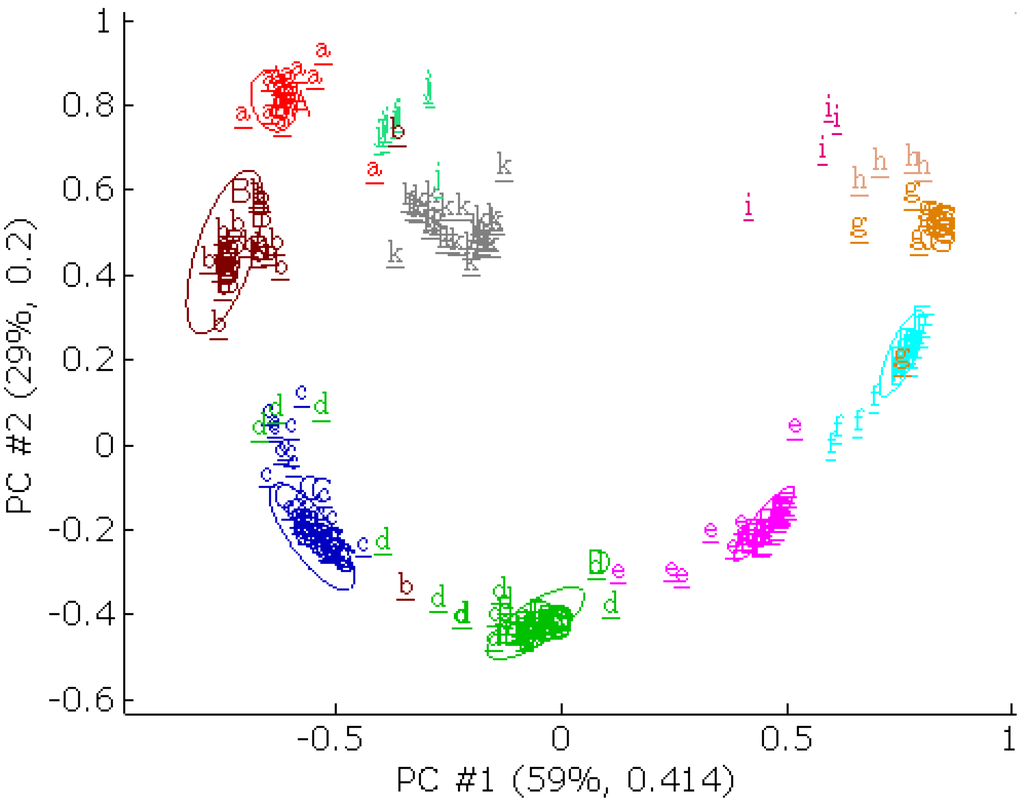
Figure 13. A principal component score plot for the PCB data set. The letters with upper case represents the training set. The underlined letters with lower case represents the external validation set. The external validation set was projected onto the first two principal components from the training set. Each axis is labeled with the percent total variance and the absolute eigenvalue from the training set. The 95% confidence intervals were calculated and given as an ellipse around each class from the training set. The PCB congeners are: (A) 2; (B) 3; (C) 4; (D) 5; (E) 6; (F) 7; (G) 8; (H) 9; (i) 10; (j) 1; (k) 0, the numbers denotes the number of chlorine atoms in the PCB congeners.

The external validation set was projected onto the first two principal components, labeled with underlined lower case letters. The external validation scores were more dispersed than the training set. A part of the external validation scores were outside of the 95% confidence interval of their class because of their low quality. The principal component scores of PCB congeners that contain 0, 1, 9 and 10 chlorine atoms were uniquely different from the training set. The BLP internal validation for the training set alone was first performed. The prediction accuracies of internal validations are given in Table 8. The average prediction accuracies of the SVM, RF, RBFCCN, and BNN models were better than the average prediction accuracy of the SCRBFN, RBFN, and PLS-DA model.

Table 8. Average numbers of correctly predicted spectra with 95% confidence intervals of PCB data set by different modeling methods with 30 BLPs.

Cl number	Total	BNN	SCRBFN	RBFN	RBFCCN
2	10	10	8.3 ± 0.5	8.0 ± 0.8	10
3	12	12	11.1 ± 0.8	11.0 ± 0.7	12
4	28	28	26.3 ± 1.5	26.1 ± 1.6	28
5	29	28.9 ± 0.1	27.1 ± 1.5	26.6 ± 1.6	28
6	24	24	23.3 ± 0.9	22.8 ± 1.4	24
7	18	18	17.0 ± 1.0	17.1 ± 1.0	18
8	10	10	9.0 ± 0.7	9.4 ± 0.6	10
Prediction accuracy (%)		99.9 ± 0.1	93.2 ± 4.6	92.4 ± 5.5	99.2
Cl number	Total	PLS-DA	SVM	RF
2	10	9.9 ± 0.1	10	10
3	12	11.9 ± 0.1	12	11.9 ± 0.1
4	28	27.5 ± 0.3	28	28
5	29	26.2 ± 0.5	29	29
6	24	22.0 ± 0.4	24	24
7	18	14.8 ± 0.6	18	18
8	10	10.0 ± 0.1	10	10
Prediction accuracy (%)		93.3 ± 0.6	100	99.9 ± 0.1

Table 8. Average numbers of correctly predicted spectra with 95% confidence intervals of PCB data set by different modeling methods with 30 BLPs.

Cl number	Total	BNN	SCRBFN	RBFN	RBFCCN
2	10	10	8.3 ± 0.5	8.0 ± 0.8	10
3	12	12	11.1 ± 0.8	11.0 ± 0.7	12
4	28	28	26.3 ± 1.5	26.1 ± 1.6	28
5	29	28.9 ± 0.1	27.1 ± 1.5	26.6 ± 1.6	28
6	24	24	23.3 ± 0.9	22.8 ± 1.4	24
7	18	18	17.0 ± 1.0	17.1 ± 1.0	18
8	10	10	9.0 ± 0.7	9.4 ± 0.6	10
Prediction accuracy (%)		99.9 ± 0.1	93.2 ± 4.6	92.4 ± 5.5	99.2
Cl number	Total	PLS-DA	SVM	RF
2	10	9.9 ± 0.1	10	10
3	12	11.9 ± 0.1	12	11.9 ± 0.1
4	28	27.5 ± 0.3	28	28
5	29	26.2 ± 0.5	29	29
6	24	22.0 ± 0.4	24	24
7	18	14.8 ± 0.6	18	18
8	10	10.0 ± 0.1	10	10
Prediction accuracy (%)		93.3 ± 0.6	100	99.9 ± 0.1

After internal validation, the entire training set was trained and the external validation set was predicted repeatedly 30 times. The prediction accuracies of external validation set are given in Table 9. The prediction accuracy without unknown is the prediction accuracy calculated by the external validation set excluding the congeners that contain 0, 1, 9 and 10 chlorine atoms. The total prediction accuracy is the prediction accuracy calculated by the complete external validation set. Because the prediction set contained low quality spectra that make the data set more difficult to classify, the result is generally worse than BLP validation. The SVM, BNN, and RF method obtained better results than other methods. The RBFCCN models yielded average prediction accuracy of 81.7% without unknown, which was ranked fifth among all the seven methods. Both the RBFCCN and SCRBFN models correctly indentified most of the unknown objects. The BNN and RBFN models were capable of classifying the test objects, but they can hardly identify the unknown objects. This result is consistent with the result from the synthetic novel class data set. As a result, the BNN and PLS models yielded total prediction accuracies lower than 65%.

Table 9. Average numbers of correctly predicted spectra with 95% confidence intervals of PCB external validation data set. All modeling methods were reconstructed 30 times. The prediction accuracy without unknown is the prediction accuracy calculated by the external validation set excluding the congeners that contain 0, 1, 9 and 10 chlorine atoms. The total prediction accuracy is the prediction accuracy calculated by the complete external validation set.

Cl number	Total	BNN	SCRBFN	RBFN	RBFCCN
2	13	13	11	12.1 ± 0.1	12
3	20	17.5 ± 0.4	17	16.6 ± 0.2	16
4	28	26.8 ± 0.4	19	24.9 ± 0.2	27
5	21	17.2 ± 0.4	20	15.5 ± 0.4	16
6	13	11.3 ± 0.3	10	11.0 ± 0.5	7
7	7	6.7 ± 0.2	5	5.0 ± 0.1	6
8	7	6	3	4.8 ± 0.4	5
0,1,9,10	45	0.3 ± 0.4	45	23.5 ± 8.3	43
Prediction accuracy without unknown (%)		90.4 ± 0.6	78.0	82.4 ± 0.5	81.7
Total prediction accuracy (%)		64.0 ± 0.5	84.4	73.6 ± 6	85.7
Cl number	Total	PLS-DA	SVM	RF
2	13	10	13	13
3	20	14	19	18.6 ± 0.2
4	28	28	28	26.3 ± 0.2
5	21	11	17	15.0 ± 0.1
6	13	8	11	11.1 ± 0.2
7	7	7	7	5
8	7	6	6	6
0,1,9,10	45	0	-	-
Prediction accuracy without unknown (%)		77.1	92.7	87.2 ± 0.4
Total prediction accuracy (%)		54.5	-	-

Table 9. Average numbers of correctly predicted spectra with 95% confidence intervals of PCB external validation data set. All modeling methods were reconstructed 30 times. The prediction accuracy without unknown is the prediction accuracy calculated by the external validation set excluding the congeners that contain 0, 1, 9 and 10 chlorine atoms. The total prediction accuracy is the prediction accuracy calculated by the complete external validation set.

Cl number	Total	BNN	SCRBFN	RBFN	RBFCCN
2	13	13	11	12.1 ± 0.1	12
3	20	17.5 ± 0.4	17	16.6 ± 0.2	16
4	28	26.8 ± 0.4	19	24.9 ± 0.2	27
5	21	17.2 ± 0.4	20	15.5 ± 0.4	16
6	13	11.3 ± 0.3	10	11.0 ± 0.5	7
7	7	6.7 ± 0.2	5	5.0 ± 0.1	6
8	7	6	3	4.8 ± 0.4	5
0,1,9,10	45	0.3 ± 0.4	45	23.5 ± 8.3	43
Prediction accuracy without unknown (%)		90.4 ± 0.6	78.0	82.4 ± 0.5	81.7
Total prediction accuracy (%)		64.0 ± 0.5	84.4	73.6 ± 6	85.7
Cl number	Total	PLS-DA	SVM	RF
2	13	10	13	13
3	20	14	19	18.6 ± 0.2
4	28	28	28	26.3 ± 0.2
5	21	11	17	15.0 ± 0.1
6	13	8	11	11.1 ± 0.2
7	7	7	7	5
8	7	6	6	6
0,1,9,10	45	0	-	-
Prediction accuracy without unknown (%)		77.1	92.7	87.2 ± 0.4
Total prediction accuracy (%)		54.5	-	-

5. Conclusions

The proposed RBFCCN network combines the concepts of RBFN and CCN. During the training of RBF hidden units, a RBFCCN applies both the initialization technique similar to that of the SCRBFN and the optimization technique of CCNs. The cascade correlation algorithm furnishes the incremental learning ability of the RBFCCN. The incremental learning ability ensures the RBFCCN automatically builds its network topology during training. Before training RBFCCNs, no prior information about network topology is required. As a result, training RBFCCNs are more convenient than training BNNs. Another advantage of cascade-correlated structure is that it avoids the moving target problem and converges more rapidly than the BNNs.

RBFCCNs, BNNs, RBFNs, SCRBFNs, PLS-DAs, SVMs and RFs were tested with four data sets. The test results were obtained with statistical measurements of confidence intervals. The SVM and RF methods proved their excellence over the neural network approaches on these classification problems. All three neural networks were generally yielded better performance than PLS-DA in prediction. Compared with the RBFN and SCRBFN models in four test data sets, the RBFCCN models generally yielded better prediction accuracies. The RBF transfer function applied in RBFCCNs makes RBFCCNs a reliable approach for novel class evaluation. RBFCCNs generally yielded better novel class evaluation ability compared with RBFNs, BNNs and PLS-DA by setting an output threshold 0.5. The RBFCCN is also capable of modeling imbalanced data set. The RBFCCN was statistically shown to be a robust and effective classification algorithm for chemometrics, especially in novel class evaluation and outlier detection.

Future work will involve in developing novel training methods to train the networks more rapidly. Investigations of different optimization algorithms such as the genetic algorithms and particle swarm optimizations to train RBFCCNs are necessary. In addition, it is important to compare RBFCCNs with other methods for outlier or novel class evaluation, such as one-class SVM in chemical data sets.

References and Notes

- Rumelhart, D.E.; Hinton, G.E.; Williams, R.J. Learning Representations by Back-Propagating Errors. Nature 1986, 323, 533–536. [Google Scholar] [CrossRef]
- Rumelhart, D.E.; Macclelland, J.L. Parallel Distributed Processing: Explorations in the Microstructure of Cognition: 1: Foundations, 2nd Ed. ed; MIT Press: Cambridge, MA, USA, 1986; pp. 318–362. [Google Scholar]
- Eiceman, G.A.; Wang, M.; Prasad, S.; Schmidt, H.; Tadjimukhamedov, F.K.; Lavine, B.K.; Mirjankar, N. Pattern Recognition Analysis of Differential Mobility Spectra with Classification by Chemical Family. Anal. Chim. Acta 2006, 579, 1–10. [Google Scholar] [CrossRef] [PubMed]
- Marengo, E.; Bobba, M.; Robotti, E.; Lenti, M. Hydroxyl and Acid Number Prediction in Polyester Resins by near Infrared Spectroscopy and Artificial Neural Networks. Anal. Chim. Acta 2004, 511, 313–322. [Google Scholar] [CrossRef]
- Fahlman, S.E.; Lebiere, C. The Cascade-Correlation Learning Architecture; Report CMU-CS-90-100; Carnegie Mellon University: Pittsburgh, PA, USA, 1991; pp. 1–13. [Google Scholar]
- Wood, M.J.; Hirst, J.D. Predicting Protein Secondary Structure by Cascade-Correlation Neural Networks. Bioinformatics 2004, 20, 419–420. [Google Scholar] [CrossRef] [PubMed]
- Diamantopoulou, M.J.; Antonopoulos, V.Z.; Papamichail, D.M. Cascade Correlation Artificial Neural Networks for Estimating Missing Monthly Values of Water Quality Parameters in Rivers. Water Resour. Manage. 2007, 21, 649–662. [Google Scholar] [CrossRef]
- Harrington, P.B. Temperature-Constrained Cascade Correlation Networks. Anal. Chem. 1998, 70, 1297–1306. [Google Scholar] [CrossRef] [PubMed]
- Chen, P.; Harrington, P.B. Discriminant Analysis of Fused Positive and Negative Ion Mobility Spectra Using Multivariate Self-Modeling Mixture Analysis and Neural Networks. Appl. Spectrosc. 2008, 62, 133–141. [Google Scholar] [CrossRef] [PubMed]
- Wang, F.; Zhang, Z.; Cui, X.; Harrington, P.B. Identification of Rhubarbs by Using Nir Spectrometry and Temperature-Constrained Cascade Correlation Networks. Talanta 2006, 70, 1170–1176. [Google Scholar] [CrossRef] [PubMed]
- Wan, C.; Harrington, P.B. Screening Gc-Ms Data for Carbamate Pesticides with Temperature-Constrained Cascade Correlation Neural Networks. Anal. Chim. Acta 2000, 408, 1–12. [Google Scholar] [CrossRef]
- Wan, C.; Harrington, P.B. Self-Configuring Radial Basis Function Neural Networks for Chemical Pattern Recognition. J. Chem. Inf. Comput. Sci. 1999, 39, 1049–1056. [Google Scholar] [CrossRef]
- Cortes, C.; Vapnik, V. Support-Vector Networks. Mach. Learn. 1995, 20, 273–297. [Google Scholar] [CrossRef]
- Breiman, L. Random Forests. Mach. Learn. 2001, 45, 5–32. [Google Scholar] [CrossRef]
- Geladi, P.; Kowalski, B.R. Partial Least-Squares Regression: A Tutorial. Anal. Chim. Acta 1986, 185, 1–17. [Google Scholar] [CrossRef]
- Frank, I.E.; Kowalski, B.R. Prediction of Wine Quality and Geographic Origin from Chemical Measurements by Partial Least-Squares Regression Modeling. Anal. Chim. Acta 1984, 162, 241–251. [Google Scholar] [CrossRef]
- Harrington, P.B. Statistical Validation of Classification and Calibration Models Using Bootstrapped Latin Partitions. Trends Anal. Chem. 2006, 25, 1112–1124. [Google Scholar] [CrossRef]
- Chang, C.; Lin, C. Libsvm: A Library for Support Vector Machines. http://www.csie.ntu.edu.tw/~cjlin/libsvm/ (accessed June 2009).
- Jaiantilal, A. Randomforest-Matlab. http://code.google.com/p/randomforest-matlab/ (accessed June 2009).
- Walczak, B.; Massart, D.L. Local Modelling with Radial Basis Function Networks. Chemom. Intell. Lab. Syst. 2000, 50, 179–198. [Google Scholar] [CrossRef]
- Clarkson University's Ftp Archive. ftp://ftp.clarkson.edu/pub/hopkepk/Chemdata/Original/ oliveoil.dat (accessed July 2008).
- Hopke, P.K.; Massart, D.L. Reference Data Sets for Chemometrical Methods Testing. Chemom. Intell. Lab. Syst. 1993, 19, 35–41. [Google Scholar] [CrossRef]
- McLafferty, F.W. Registry of Mass Spectral Data, 5th Ed. ed; John Wiley & Sons: New York, NY, USA, 1989. [Google Scholar]
- Crawford, L.R.; Morrison, J.D. Computer Methods in Analytical Mass Spectrometry. Identification of an Unknown Compound in a Catalog. Anal. Chem. 1968, 40, 1464–1469. [Google Scholar] [CrossRef]
- Tandler, P.J.; Butcher, J.A.; Hu, T.; Harrington, P.B. Analysis of Plastic Recycling Products by Expert Systems. Anal. Chim. Acta 1995, 312, 231–244. [Google Scholar] [CrossRef]
© 2009 by the authors; licensee Molecular Diversity Preservation International, Basel, Switzerland. This article is an open-access article distributed under the terms and conditions of the Creative Commons Attribution license (http://creativecommons.org/licenses/by/3.0/).