A Survey on Star Identification Algorithms

Abstract

The author surveys algorithms used in star identification, commonly used in star trackers to determine the attitude of a spacecraft. Star trackers are a staple of attitude determination systems for most types of satellites. The paper covers: (a) lost-in-space algorithms (when no a priori attitude information is available), (b) recursive algorithms (when some a priori attitude information is available), and (c) non-dimensional algorithms (when the star tracker calibration is not well-known). The performance of selected algorithms and supporting algorithms are compared.

1. Introduction

The requirement for attitude (orientation) information of a spacecraft has been the mother of invention of many devices and algorithms, notably the process of autonomously identifying stars (Star-ID). Though there is much history of devices used to identify stars and compute an attitude that do not use a star camera, this paper primarily analyzes algorithms that use a star camera with an imaging array and an algorithm to match observed (body) directions of stars with catalog (inertial) directions of stars without requiring reorienting the camera or the spacecraft. These algorithms fall into two basic categories, lost-in-space algorithms, in which no information regarding the attitude of the spacecraft is available, and recursive algorithms, in which some information regarding the attitude is available. These techniques typically use inter-star angles (the angle between the line-of-sight of two stars from the perspective of a camera), the brightness of the stars, and some computations of these values to distinguish stars. A further subcategory of both categories is non-dimensional Star-ID, in which the exact angular separations are not required but the values are normalized to be insensitive to poor camera calibration, or time-varying camera calibration parameters [1,2,3].

Figure 1. Typical Star-Tracker Image-based Attitude Determination Flow.

Figure 1. Typical Star-Tracker Image-based Attitude Determination Flow.

Star-ID is just one step in the process of determining the attitude of a spacecraft, as depicted in Figure 1. The first algorithms in the sequence measure body-frame vectors for the locations to observed stars. The Star-ID process has as its primary purpose determining the inertial-frame vectors for some or all of the body-frame vectors given to it. Subsequent algorithms determine a suitable transformation that correctly maps the body vectors to the inertial vectors, thereby calculating the spacecraft’s attitude. When sensing the stars with a CCD imaging array, the information available for the identification process is the brightness of the star and the angular separation between stars.

Figure 2. Typical Star-ID Process.

Figure 2. Typical Star-ID Process.

Star-ID task has three basic pieces, with an optional fourth, as illustrated in Figure 2. First, an algorithm must extract features from a set of body vectors and associated brightness. Second, a database search matches a subset of the observations with entries in the database, and third makes some estimate as to the probability that they are correct. Optionally, the remaining body vectors are identified once an estimate of the attitude is available in a method called “recursive” Star-ID. This fourth step typically implements a variation of the “direct match” technique in which stars are identified by their close proximity to their predicted location. The recursive mode is typically much faster than the first two, and can usually be repeated successively for additional observations with an a priori estimate of the attitude.

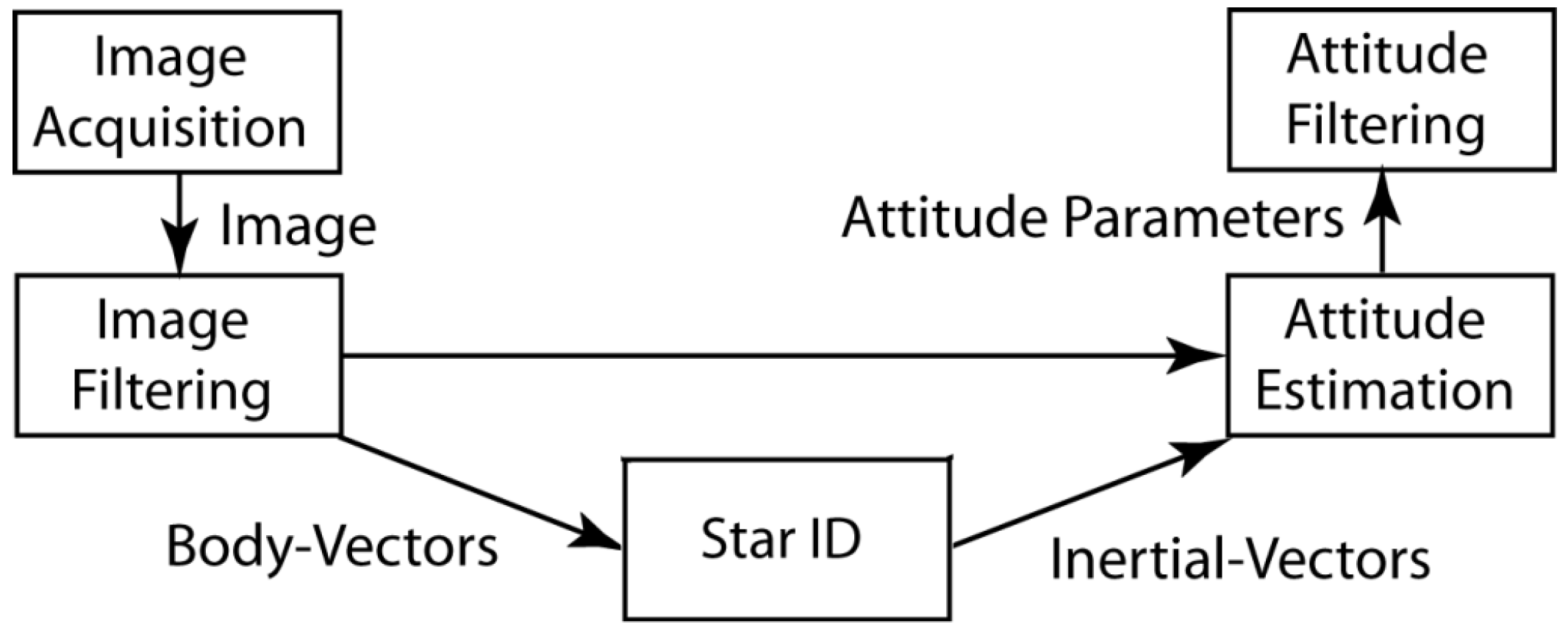
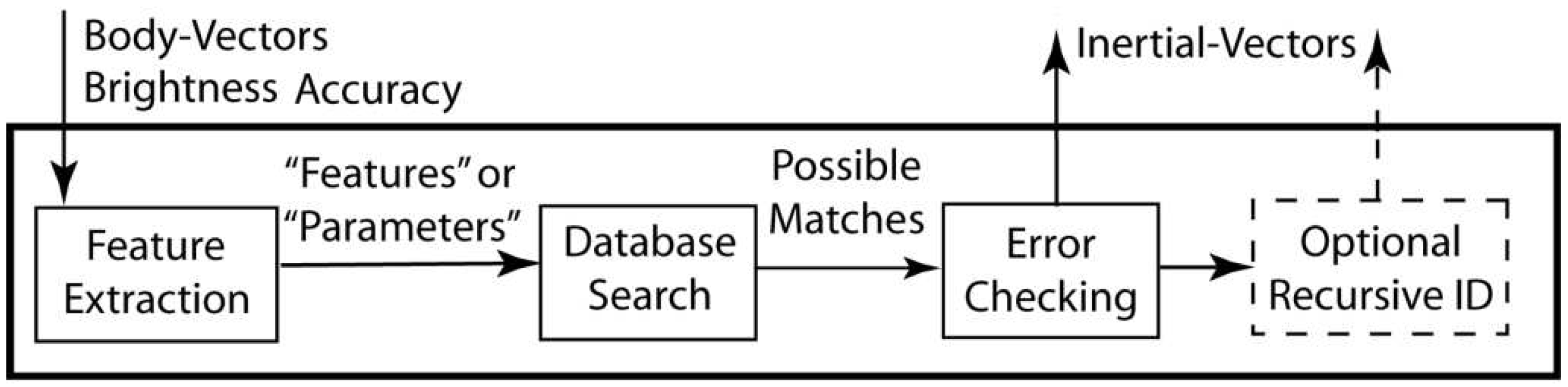
1.1. Topics Covered, Notation, and Figures

The algorithms surveyed in this paper are evaluated by the analytical asymptotic performance of

• the feature extraction step,
• database search, and
• their utilization of independent pattern features in the star features based on how many stars are used in a pattern.

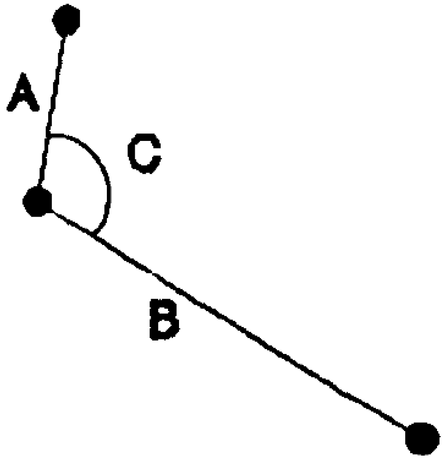
For all cases, the number of stars referenced in the star catalog is n, the average number of stars observed in the field of view of the camera is f, and the number of stars in a pattern is b. Although a star pattern containing b stars has ${\displaystyle \frac{b(b-1)}{2}}$ inter-star angles which may be measured, the number of independent pattern features for a star pattern of b stars, is only ($2b-3$), since some inter-star angles are dependent on the values of others. By including star magnitude information, which is typically much less precise than inter-star angle information, an additional b independent pattern features may be used. Throughout this paper, the use of asymptotic notation, $O(\dots )$, is used to indicate the highest order term in the running time of an algorithm. Algorithms are analyzed based on the described implementation in the referenced papers. Any assumptions drawn about their performance time, when not directly stated in the paper, is based on the progression and availability of certain algorithms at the time, although alternative running times are discussed if it seems likely they could have been implemented. Furthermore, the common computer science notation, “$lgn$” is used to mean “${log}_{2}n$”.

To preserve the original authors’ intent, the figures shown here are duplicated from the referenced papers.

2. The Beginning

After the first CCD-based star tracker was developed by Salomon in 1976 at JPL [4], Junkins, Turner, Strikwerda [5,6], and others began work on implementing an algorithm that could identify stars in real-time. While they realized the benefit of using the easily-computable sine of inter-star angles as a pattern feature, the key problem that arose was the matching of observed inter-stars to the items in the database. After several years of work and a few conference papers, Junkins et al. published “Star Pattern Recognition and Spacecraft Attitude Determination” in 1981 [7]. Although the algorithm was able to identify star triplets, it had the primary limitation of requiring an a priori estimate of the spacecraft’s attitude before it was able to perform in real-time. The reason is that Junkins had used “sub catalogs” of the sky, illustrated in Figure 3, each representing a portion of the sky, in order to accelerate the computation. Although the method was robust to non-stars because the catalog included all combinations of stars that might be observed, it only updated the attitude estimation algorithm once or twice a minute, as contrasted with the angular rate sensors, which updated at $\mathrm{1,000}$ times per minute. The majority of the attitude estimation was propagation of the angular rate sensors, and periodic checks were established to confirm and improve the propagated attitude. Junkins’ feature extraction runs very fast, in $O\left(b\right)$ time, since it may select any three of the observed stars and measure the sine of their inter-star angles. However, since his database search considers every possible permutation of stars available in a given region of sky, the search time is $O\left(f^3\right)$, where f is the number of stars in a given sub-catalog, usually the same size of a given field of view. The time to perform Star-ID increases if the stars are not located in the predicted field of view as other sub-catalogs are searched. The database itself would grow as $O\left(n{f}^2\right)$.

Figure 3. Field-of-view-sized sub-catalogs (reprinted from [7]).

Figure 3. Field-of-view-sized sub-catalogs (reprinted from [7]).

In 1986, Groth [8] suggested that a faster way to search the sub-catalogs would be to sort the triangles sides in order based on permutation-invariant values such as the logarithm of the perimeter of a triangle. He admits, however, that his algorithm runs at high polynomial power of n, much as Junkins’ has. Groth’s algorithm differs in that the performance has a lower constant factor. While the asymptotic order of the database is identical to Junkins, there would be more data included, associated with the permutation-invariant values.

In 1987, Sasaki [9] and others published a patent showing how to improve the search time by using the area of a star triangle and the sum of the luminous intensities as preliminary markers in performing the star identification, using $O\left(b\right)$-time for star feature extraction. His method does not discuss the way in which the database is searched, requiring only that a “number of stars” will be selected from the database by a method using “parallel, serial, or the like” processors. It is not noted whether his database indeed contains as many star triplets as does Junkins’ method, nor is the search procedure described.

Later, in 1989, Van Bezooijen [2] suggested in his dissertation that the speed of the star pattern recognition algorithm could be improved by making more use of the available information in the star patterns. Van Bezooijen discussed directly the relationship between the number of stars and the amount of information available from a star pattern with a given number of stars. His analysis also included a very detailed statistical probability that a star had been identified correctly. Unfortunately, Van Bezooijen’s method sometimes required the spacecraft to slew in order to detect stars for his Star-ID method, and as such, his work is not covered in depth here.

In 1991, with Junkins on his advisory committee, David Anderson [10] addressed the ambiguity of the order of star triplets by proposing a permutation matrix, and the development of star pattern parameters that were independent of the order in which the stars are selected. Sticking with the tried-and-true star-triple pattern, Anderson also proposed the use of an array processor to handle the matrix multiplications required to use his permutation matrices. Unfortunately, the database storage remained $O\left(n{f}^2\right)$, and there was no advance made on the database search. Anderson suggested that an array processor be used to perform the matrix multiplication, decreasing the running time of the Star-ID process. The design engineer should note that array processors, while performing a comparatively large number of computations when contrasted with a serial processor, also use a comparatively large amount of power, because they both tend to use identical amounts of energy to perform each computation.

3. Search Process Acceleration

The next year, Liebe [11] made the critical connection of the feature selection process to the database search time, making the Lost-In-Space problem tractable. Liebe suggested the use of the two closest stars to a selected star as components of the star pattern, and the angular separations from the two closest stars and the angle between them as his parameters, as illustrated in Figure 4, and addressed the situations in which predicted stars would not be seen due to their magnitude being very close to the detection threshold. Liebe also address the situation in which small errors would cause the incorrect selection of the closest two stars when the distance to these stars were similar. Although Leibe’s feature extraction process now took $O(flgb)$-time to compute, his database could be reduced to $O\left(n\right)$, and subsequently, his database search could be performed much faster, though still linear-time. Liebe makes full use of the available angular independent pattern features, neglecting the stellar magnitudes. Liebe later implements the optional recursive direct match mode which could identify the remaining stars up to 20 times faster than the Lost-In-Space algorithm.

Figure 4. Liebe’s parameters, 2 inter-star angles and 1 interior angle (reprinted from [11]).

Figure 4. Liebe’s parameters, 2 inter-star angles and 1 interior angle (reprinted from [11]).

Then in 1993, Baldini [12] proposed a multi-step Star-ID method. Baldini’s method identifies the brightest b stars in a given image, requiring $O(flgb)$ time. He then measures the angular separation of the sequence of five stars, $O\left(b\right)$ time. Baldini then proceeds through a linear search of the catalog search for every star in the catalog which falls within an acceptable tolerance range of the observed stars, requiring $O\left(bn\right)$-time, neglecting the time for dynamic list creation, although this step would be improved by other algorithms in the future. If we use the expression $\Delta m$ to represent the fraction of stars in the catalog that fall within the acceptable range, he has an intermediate result of $O(\Delta mn)$ stars in each of b lists. He then compares the distance of each star in adjacent lists determining if any star cannot have an angular separation within the tolerance of the observed angular separation, requiring $O\left(b{(\Delta mn)}^2\right)$-time, although as he points out, as items are eliminated the number of comparison at each iteration is reduced. Baldini is then left with b lists containing stars that meet their neighboring distance criteria, he then forms all combinations of the stars, discarding combinations whose sequence of angular separations does not match the observed stars. The running time of this step is represented analytically by $O\left(a^b\right)$, assuming there are approximately a stars in each of b lists. It is certain that the rejection of certain combinations in the second or third step is sure to reduce the total number of comparisons, and Baldini is certain to conclude with only one or two possible combinations of stars. Baldini has used five stars, inherently containing twelve independent features, but uses only nine when performing his identification process, suggesting the required field of view may be larger for Baldini’s method when compared to other methods to be sure that there will be enough visible stars. Although non-stars will get weeded out in the process, the addition of non-stars to the algorithms increases most of the steps linearly or quadratically.

In 1995 Ketchum [13] proposed a second sequential filtering algorithm, this time using the brightness of the brightest star to attempt to determine the likelihood of pointing in any particular direction. She then filters the list of possible stars using the brightness of the second brightest star. Although she admits the algorithm would need to search as much as 43% of the catalog for the appropriate stars, she notes that the storage space required by his algorithm is much less than required by Van Bezooijen’s method. Furthermore, Ketchum is one of few to give direct empirical data regarding the running-time of his algorithm, reporting it requires up to 63 seconds to run on a 50 MHz processor.

Later in 1995, Scholl [14] published a more straightforward method. The inter-star angles were to be ordered by their relative brightness, eliminating the permutations that arise when considering the possible orders of three stars. Unfortunately, Scholl retains the $O\left(n{f}^2\right)$-sized catalogs, and does not specify the search technique used. While it’s true that his method uses less time to search the database when compared to Baldini, it is nonetheless still $O\left(n{f}^2\right)$, since faster techniques were not proposed until the following year.

3.1. Search Time Dramatically Reduced

In 1996, Quine [15] was the first to attack the database search problem head on, realizing that a binary search tree (see Figure 5) could be used to search the database in $O(lgn)$-time. He retains Liebe’s use of the two closest stars to a given star to form a pattern, resulting in a database of size $O\left(n\right)$, instead of previous catalogs that used all observable combinations of stars. While this increases his feature extraction time to $O(flgb)$, the trade off is quite advantageous for large values of n.

Figure 5. Quine’s Binary Tree (reprinted from [15]).

Figure 5. Quine’s Binary Tree (reprinted from [15]).

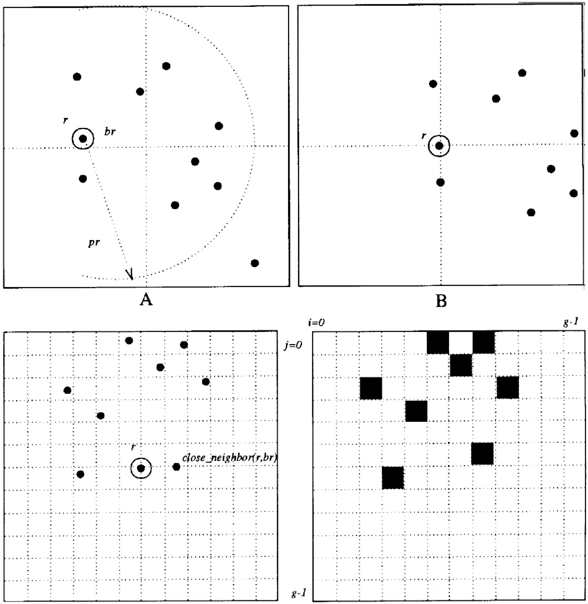
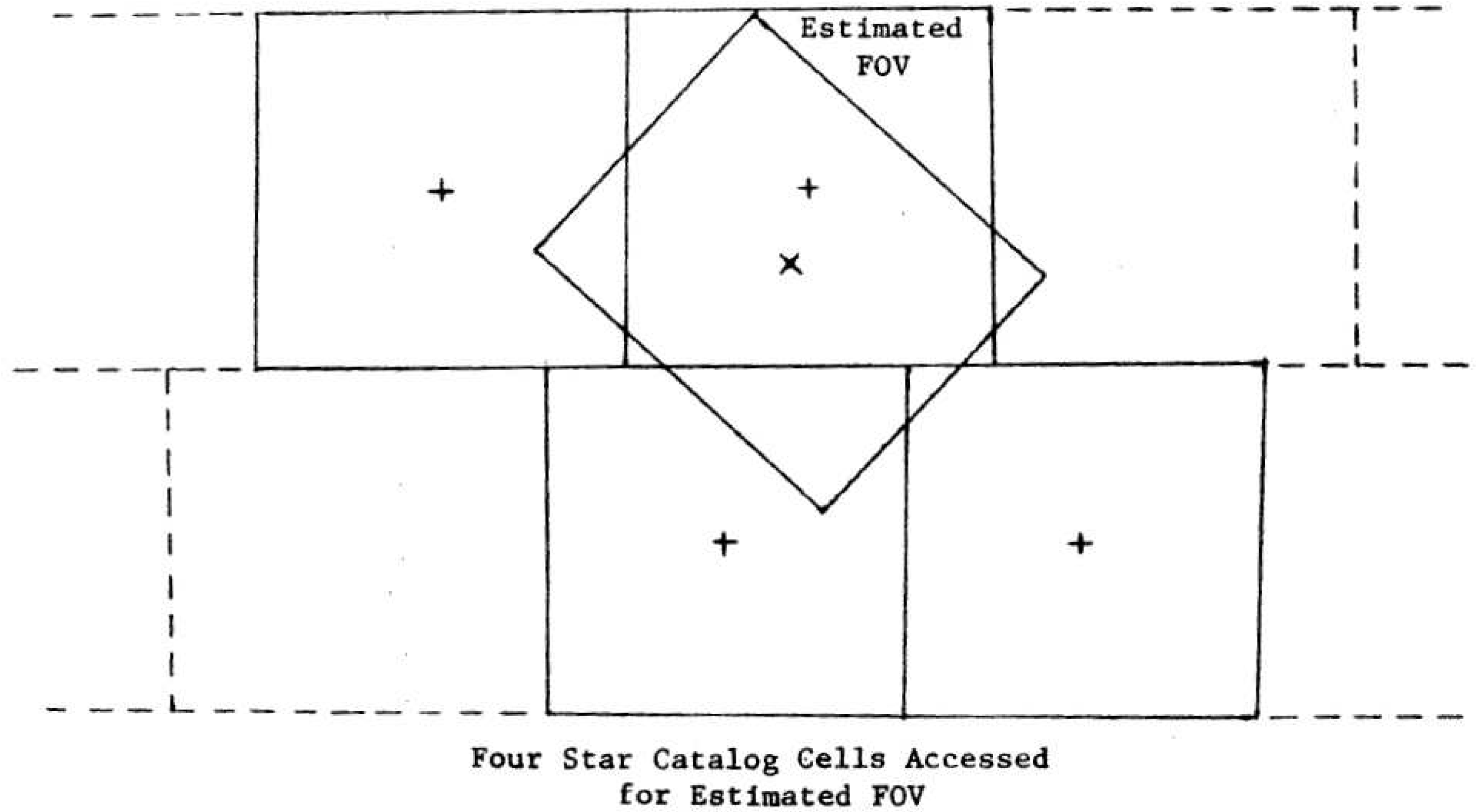
3.2. Novel Grid Algorithm

In 1997, Padgett [16] published perhaps the first novel star pattern recognition algorithm, which actually used a star “pattern.” Padgett’s grid algorithm cast the locations of neighboring stars as items on a loose grid (see Figure 6). Padgett solved the roll ambiguity by rotating the observed stars about a given star until the nearest star to the given star was aligned with the x axis. The cells in the grid were then considered to be “on” if there was a star located inside it, and “off” if there were not. The locations of the “on cells” then become the features, the indexes of the “on cells” were listed as items in a vector. His feature extraction time became $O\left(f\right)$. Unfortunately, Padgett was unable to improve the database search time for his features beyond linear, and the resulting database search remained $O\left(n\right)$. Further analysis indicated that Padgett’s method was quite robust to the presence of non-stars owing to its large grid cell size when compared to the angular error in star position.

Figure 6. Illustration of Padgett’s Grid Algorithm (reprinted from [16]).

Figure 6. Illustration of Padgett’s Grid Algorithm (reprinted from [16]).

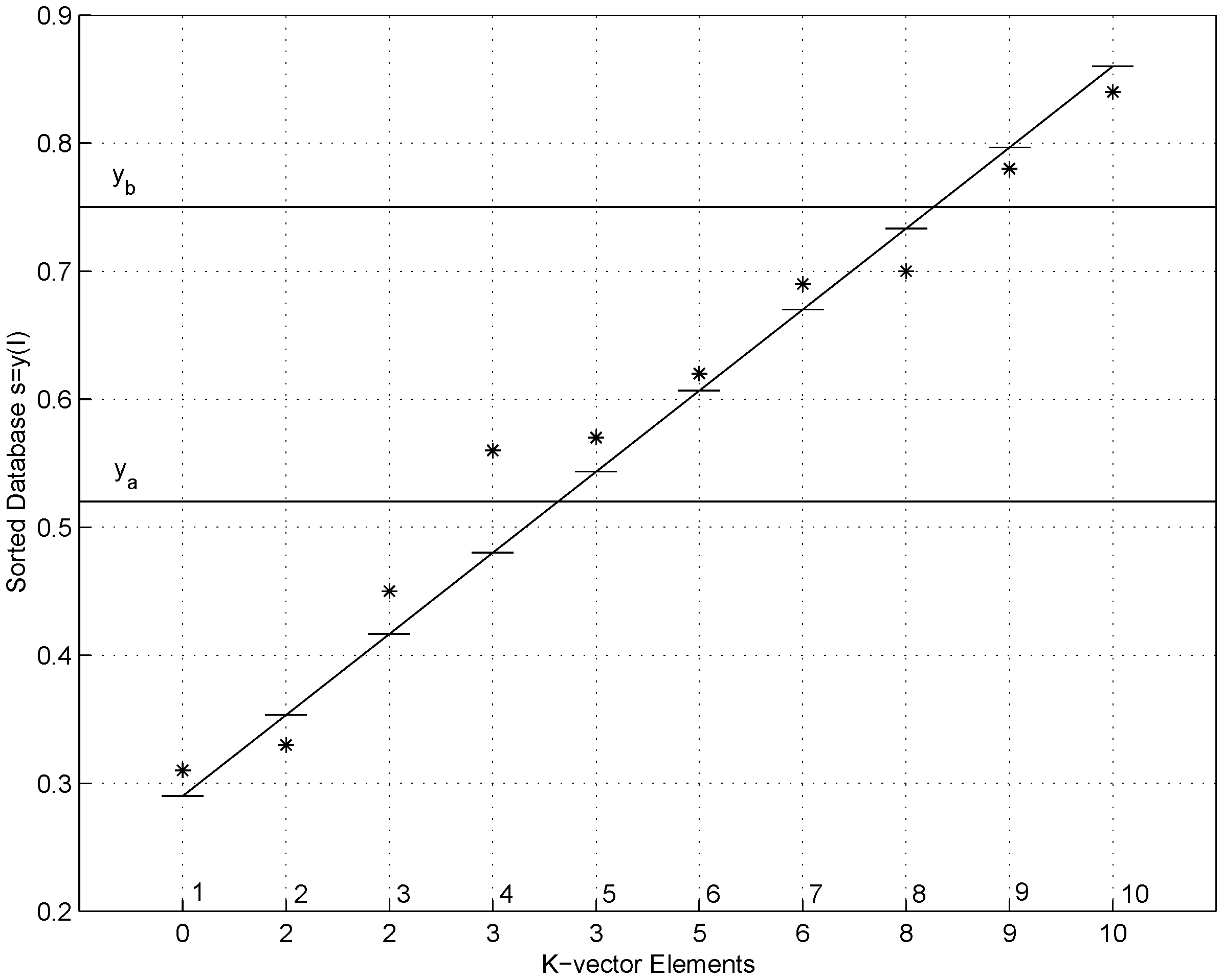
3.3. Search Time Reduced Much Further

Later in 1997, Mortari [17,18] proposed an even faster database search technique, the “Search-Less Algorithm,” (SLA). Mortari retained the approach of selecting any pair of stars in the field of view, $O\left(b\right)$-time, but he proposed using a “k-vector” to search the database in an amount of time independent of the size of the database [19]. Figure 7 shows the k-vector construction for a 10-element database. The small horizontal lines are equally spaced and they give the k-vector values: $0,2,2,3,3,5,6,8,9,10$.

Figure 7. Example of k-vector construction (reprinted from [19]).

Figure 7. Example of k-vector construction (reprinted from [19]).

The search time for a single star-pair would be $O\left(k\right)$, where k is the number of possible star pairs with inter-star angles within the measurement tolerance. Unfortunately, the dominant time of the algorithm came when comparing multiple lists of stars returned for each inter-star angle. Since multiple stars had to have all their inter-star angles confirmed to be a match, the running time of the comparison would be $O\left(b{k}^2\right)$, and b is the number of stars in the pattern required to guarantee uniqueness. Even though the resulting value of k would be a number based on the uncertainty associated with the inter-star angle measurement and the number of observable star pairs, Mortari had made the first important step in breaking the dependence of the database search time on the size of the database. Mortari’s method could also reject a single non-star from a set of selected stars, without loosing the progress made in identifying the others. The resulting Search-Less Algorithm (SLA) was then successfully tested on orbit on an Indian satellite [20].

A few years later, realizing that the robustness to non-star “spikes” was essential towards reducing the number of iterations of his algorithm, Mortari developed the “Pyramid” algorithm [21] which uses an optimal permutation algorithm to exploit the ability of his algorithm to select which stars to match. This permutation is written to minimize the time spent considering stars that don’t match, fearing them to be non-star spikes. The code has been tested to reject non-stars in an image containing only five real star but with 63 non-stars thrown in. The Pyramid algorithm has been successfully tested on Draper’s “Inertial Stellar Compass” star tracker [22] and on MIT’s satellites HETE and HETE-2 [23]. This algorithm is presently under exclusive contract to StarVision Technologies.

Neural networks, have been proposed for use in Star ID as early as 1989, [24]. In 2000, Hong [25], proposed using a neural network and fuzzy logic to identify the stars, as illustrated in Figure 8. Hong used the popular ordered triple, based on star brightness, and fed the resulting angular separations into a neural network. While his feature extraction process runs very fast, $O\left(1\right)$, he is forced to use a massively parallel architecture to implement the neural network. Though such techniques may be used with much success on ground-based systems, it is uncertain if this technique is the best for use in a system with limited electrical power, or that requires expensive radiation-tolerant hardware. Hong notes quite accurately that his algorithm performs much faster than some other of the mentioned algorithms, referencing Van Bezooijen, Quine and Ketchum, but failed to make a comparison with Mortari’s method. Hong readily admits that his technique requires more than a quarter-million multiplications.

Figure 8. Hong’s Neutral Network (reprinted from [25]).

Figure 8. Hong’s Neutral Network (reprinted from [25]).

Then in 2007, Guangjun [26] proposed a feature extraction technique, similar to Liebe [11], using the inter-star angles and the angle made by two stars relative to a central star. Though his feature extraction time is $O(flgb)$, he uses a linear database search, performing bit-by-bit comparisons, running in $O\left(n\right)$ time. While Guangjun’s claim [26] is true that his algorithm runs faster than Padget’s grid algorithm [16], similarly to Hong [25], he fails to compare his algorithm to more-recent faster algorithms.

In 2008, Kolomenkin [27] proposed a modification of the SLA algorithm to reduce the time spent cross-checking the results of the k-vector. In the original SLA algorithm, Mortari selects any four stars in the image and performs six k-vector searches to find six lists of approximately $k=100$ candidate star pairs. The cross checks take $O\left(k^2\right)$-time, and this cross-check step is the bulk of the time used by the SLA algorithm. Kolomenkin suggests, however, finding all lists of all possible stars in the image (which is $O\left(f^2\right)$-searches) and maintaining a list of the number of times each visible star is listed in a particular search result, $O\left(fk\right)$ items). Once all the inter-star angles have been determined and the stars voted, the visible-catalog star match with the largest number of votes is considered to be the correct answer, and the results are filtered from there. This latest step would have running time $O\left(fk\right)$. While the algorithm does perform the cross check $O(k/f)$ faster than the SLA, it calculates $O\left(f^2\right)$ more inter-star angles, and k-vector searches, each of which takes $O\left(k\right)$-time, contributing an increase of $O\left(k{f}^2\right)$-time. For the purpose of this analysis, the time for list insertion for keeping track of voting is assumed to be $O\left(1\right)$, though in practice it is difficult to perform this step in less than $O(lgk)$-time. So Kolomenkin’s modification would run asymptotically faster in systems for which $f^2<k$. Since, in a given system, f tends to be on the order of 10 to 40 and k on the order of 100, it seems dubious the algorithm achieves any real decrease in asymptotic running time, most likely if any improvement is achieved, it is by a constant factor. In the paper, Kolomenkin did not provide any direct performance comparison to the unmodified SLA.

For the reader’s convenience, the major advances in asymptotic performance of Star-ID are listed in Table 1.

Table 1. Summary of Advances in Asymptotic Performance.

Author	Year	Feature	Database	Database	Validation	Used
		Extraction	Size	Search		measurements
						/Available
Junkins	1981	$O\left(b\right)$	$O\left(n{f}^3\right)$	$O\left(f^3\right)$	N/A	3/3
Liebe	1992	$O(flgb)$	$O\left(n\right)$	$O\left(n\right)$	N/A	3/3
Baldini	1993	$O(flgb)$	$O\left(nb\right)$	$O\left(b{(\Delta mn)}^2\right)$	$O\left(a^b\right)$	9/12
Scholl	1995	$O(blgb)$	$O\left(n{f}^2\right)$	$O\left(n{f}^2\right)$	$O\left(k\right)$	6/6
Quine	1996	$O(flgb)$	$O\left(n\right)$	$O(lgn)$	N/A	6/6
Padgett	1997	$O\left(f\right)$	$O\left(n\right)$	$O\left(n\right)$	N/A	$2f/2f$
Mortari	1997	$O\left(b\right)$	$O\left(nf\right)$	$O\left(k\right)$	$O\left(b{k}^2\right)$	6/6
Kolomenkin	2008	$O\left(b\right)$	$O\left(nf\right)$	$O\left(k\right)$	$O\left(k{f}^2\right)$	6/6

Table 1. Summary of Advances in Asymptotic Performance.

Author	Year	Feature	Database	Database	Validation	Used
		Extraction	Size	Search		measurements
						/Available
Junkins	1981	$O\left(b\right)$	$O\left(n{f}^3\right)$	$O\left(f^3\right)$	N/A	3/3
Liebe	1992	$O(flgb)$	$O\left(n\right)$	$O\left(n\right)$	N/A	3/3
Baldini	1993	$O(flgb)$	$O\left(nb\right)$	$O\left(b{(\Delta mn)}^2\right)$	$O\left(a^b\right)$	9/12
Scholl	1995	$O(blgb)$	$O\left(n{f}^2\right)$	$O\left(n{f}^2\right)$	$O\left(k\right)$	6/6
Quine	1996	$O(flgb)$	$O\left(n\right)$	$O(lgn)$	N/A	6/6
Padgett	1997	$O\left(f\right)$	$O\left(n\right)$	$O\left(n\right)$	N/A	$2f/2f$
Mortari	1997	$O\left(b\right)$	$O\left(nf\right)$	$O\left(k\right)$	$O\left(b{k}^2\right)$	6/6
Kolomenkin	2008	$O\left(b\right)$	$O\left(nf\right)$	$O\left(k\right)$	$O\left(k{f}^2\right)$	6/6

4. Non-dimensional Algorithms

In 2003 Samaan, along with Junkins and Mortari [3], presented a new Star-ID technique that was robust to calibration errors. For flight systems in which temperature variations would cause cyclic variations in the accuracy of the calibration, the new technique would promise to eliminate the ambiguity in matching star patterns. Instead of using the inter-star angles between stars in a triangle, Samaan used the triangle’s interior angles, the angle between two stars, with a third star as a vertex. While the inter-star angles respond linearly to changes in temperature, the triangle interior angles are invariant in the first order of the distortion, as illustrated in Figure 9. Samaan’s technique uses the smallest and largest of the interior angles to place stars in a catalog, so the feature extraction time is $O(lgb)$. The database is subsequently searched with Mortari’s k-vector searching technique, taking $O\left(k\right)$ time. Samaan’s numerical tests found that at least five stars must be matched before the technique produces, which introduces a cross-checking routine, using $O\left(b{k}^2\right)$-time. Samaan concludes the paper by using Star-ID to re-calibrate the camera.

Figure 9. Distortion from calibration variations (reprinted from [3]).

Figure 9. Distortion from calibration variations (reprinted from [3]).

Rousseau also published a method in 2005 [28], which he billed as being robust to errors introduced by new CMOS Active Pixel Sensors (APS). His metric is the sine of star-triangle interior angles, but instead of using any combination of stars, he used only the closest two stars, and used only one of the three (two independent) interior angles as a parameter. His pattern selection pattern means there is only one entry in the catalog for each star; so his catalog size is $O\left(n\right)$. It also follows that the feature extraction time is $O(flg2)=O\left(f\right)$. Furthermore, Rousseau does not specify a method for selecting star triangles from the catalog, but according to his published parameter distribution, the fastest method available would be a binary-tree search, taking $O(klgn)$-time. Rousseau then actually computes the attitude for each star triangle, and finds all the stars from the catalog that should be visible, which should take no less than $O\left(f\right)$, and more likely $O(flgn)$. Each observation is then transformed into the reference frame. The observed stars are then matched up with catalog stars, and the inter-star angles compared. The process by which this is done is not described, but likely takes $O(flgf)$-time. The best of the matches of all the triangles is then selected. The final analytic time of Rousseau’s algorithm is then $O(kflgflgn)$. It is unclear whether Rousseau’s performance data is on his original 45,000-star catalog, or another mentioned, reduced 1,300-star catalog, but his timed results are disappointing; all of his averages are longer than a second on a 650 MHz processor. Although the tests are performed in MATLAB, which unnecessarily increases the computation time, it is unclear why Rousseau claims the algorithm is fast from his reported data, and without any performance comparison to any other algorithm. Furthermore, he does not describe why his validation phase, which uses inter-star angles to reject incorrect matches, is more robust to APS-induced measurement errors, when the same inter-star angles are used by previous methods, like SLA. It seems likely that he simply used the smaller star catalog, in which larger measurement errors result in fewer incorrect matches. Rousseau’s parameters, however, have the benefit that there is no ambiguity as to which star in the triangle is the listed star, as long as the star triangle does not contain nearly identical angles.

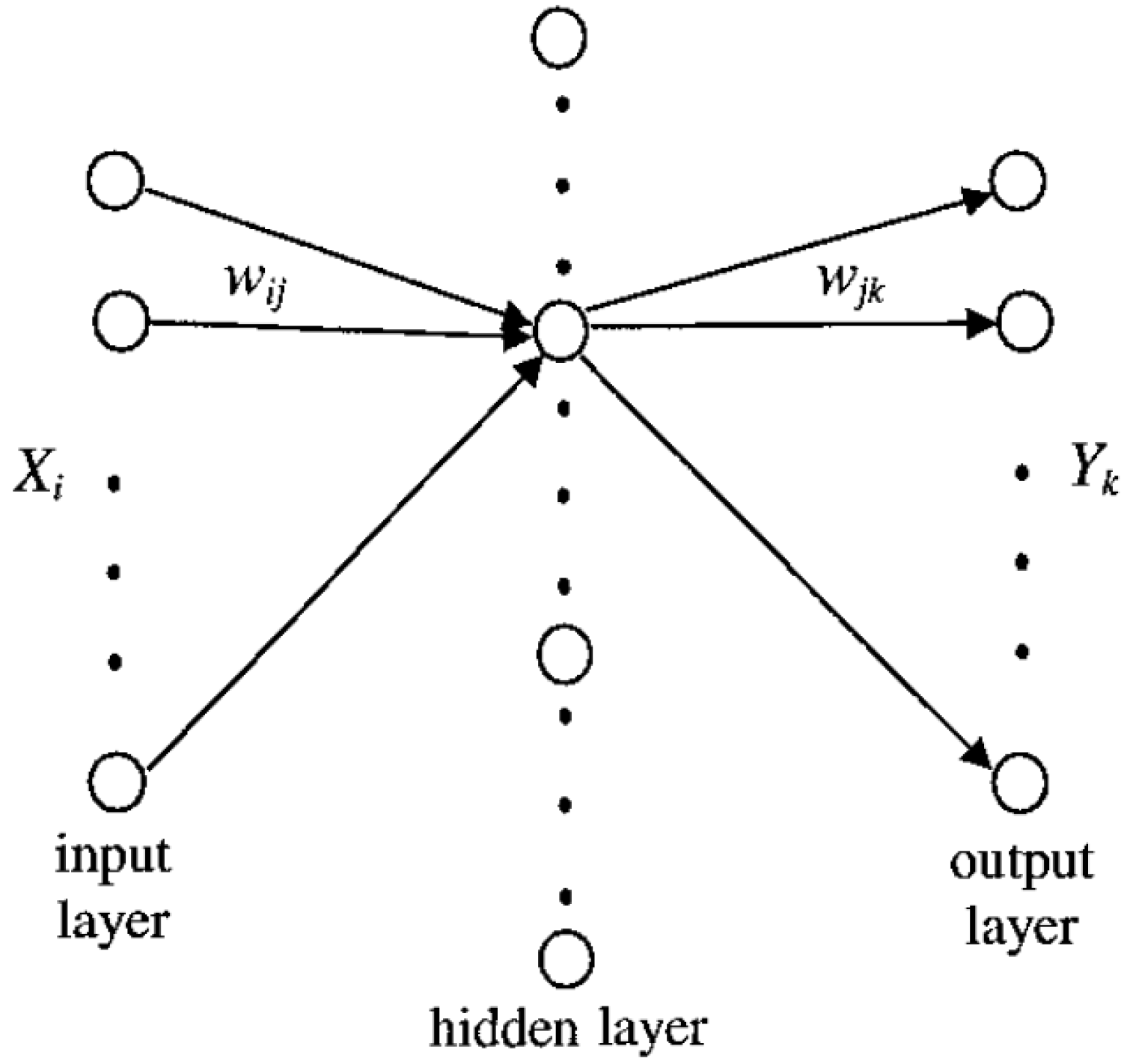
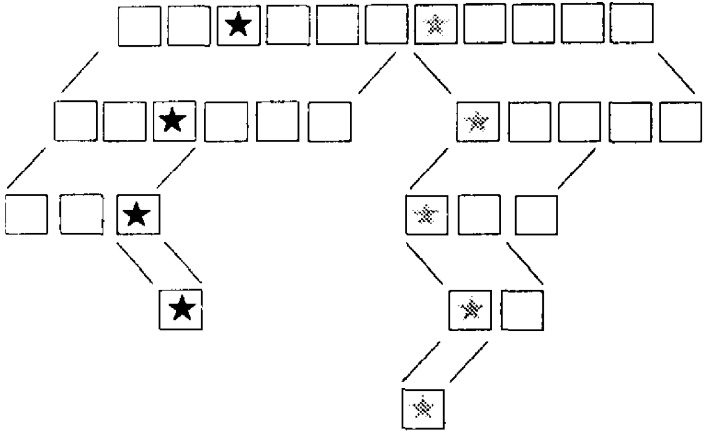
5. Recursive Star Identification

Samaan made other advances for recursive Star-ID in 2005 [29]. His key to reducing the recursive mode time was to speed the selection of stars that ought to be visible given some other visible stars. He presented two methods, one which used the Mortari’s Spherical Polygon-Search (SP-Search) [30,31], which in turn used his k-vector, and the second which used a pre-built catalog of stars that should be visible if another star is visible, the Star Neighborhood Approach (SNA). The SP-Search uses a k-vector 3 times to find the stars within calculated x, y, and z ranges in inertial space. By finding stars in common in the three resulting lists, Mortari produces a list of stars that should be visible. Each of the three database searches takes $O\left(k\right)$ time, while the cross-comparison takes $O\left(k^3\right)$-time. Samaan then uses the attitude estimate to search for the presence of these predicted stars in the set of the camera’s observed stars. Samaan’s other method, the SNA, constructs a table ahead of time, of the six closest stars to any given star, presuming these stars to be the most likely to be visible if the first star is found. Samaan’s method takes $O\left(b\right)$-time to find candidate stars, if b stars are identified by the LISA. It is uncertain how many successive iterations would be necessary to ensure that all the stars in the given field of view have been found, other than it is most likely bounded by $O\left(fb\right)$.

Star Trackers for Different Applications

Although Star-ID is predominantly used for attitude determination, it can be used for other spacecraft related tasks. Here are some examples:

• Star Gyros. With appropriate algorithms, images from star cameras may also be used for estimating the angular velocity of the spacecraft [32].
• Space Surveillance. It can be used for space situational awareness to estimate the orbit of other visible spacecraft [33,34,35].
• Space Navigation. If placed on an interplanetary probe, it could observe visible planets and estimate the location of the probe [36,37].
• Positioning System. If carried on a planet or moon, it could be used to estimate its position on the body when combined with a clock and two inclinometers [30,31].

Interesting research have been carried out to increase star sensor accuracy as well as to simplify the Star-ID problem. Here are two examples:

• Multiple Fields-of-View system. While attitude determination from a single star camera image produces very accurate information about the direction of the camera boresight, the estimate of the rotation about the camera’s boresight axis is less accurate. In order to solve this problem, a second star camera is sometimes used. There is another method, which uses a single star camera to record a combination of multiple star images simultaneously. For a two fields-of-view camera the light are preferentially smeared by the optics (e.g., by adding astigmatism) so that stars from one aperture are smeared in a horizontal direction in the image plane, while light from the other aperture is smeared in the vertical direction [38,39]. Image filtering algorithms can detect the direction of the smearing and separate the stars according to which aperture they entered. If, however, the Star-ID technique is very robust to the presence of non-stars, the Star-ID algorithm may be run many times on the same image, perhaps on stars from three apertures, all in orthogonal directions [40,41,42]. In these cases it is possible to separate the stars without the need for smearing the stars in a given direction.
• Techniques requiring multiple images as well as attitude maneuvers have been implemented [43].
• Uniform Star Catalog. In order to develop optimized star sensing and star identification with respect to continuous operation and reliability, the concept of star catalogs with near uniform angular spacing between stars has been proposed [44]. These catalogs are not characterized by constant magnitude cutoffs. They are reference star catalogs where the expectation of the number of stars that fall in a given field of view is approximately constant (i.e. 5 or 6) (minimum standard deviation), independently which region of the sky the sensor optical axis is pointing.

6. Conclusion

Through the past three decades, steady advancements have been made by various authors, employing many techniques for autonomous Star-ID. Although many complex arrangements have found to be successful, the trend for faster and more reliable methods saw rapid advancement in the 1990’s. Star-ID techniques tend to fall in one of four categories separated by two decisions: whether or not to use star brightness information, and whether to select any stars for a given star pattern or use ordinal information from brightness or distance. Once the goal of solving the Lost-In-Space case from a single image in real-time became possible without a priori information, advancements in the Star-ID field turned towards improving the robustness of Star-ID to errors in detecting stars and measuring their features.

References and Notes

1. Gottlieb, D. M. Star Identification Techniques. In Spacecraft Attitude Determination and Control; Kluwer: Dordrecht, The Netherlands, 1978; Chapter 7.7; pp. 259–266. [Google Scholar]
2. Bezooijen, R. W. H. V. Automated Star Pattern Recognition. Ph.D. Thesis, Stanford University, 1989. [Google Scholar]
3. Samaan, M. A.; Mortari, D.; Junkins, J. L. Nondimensional star identification for uncalibrated star cameras. J. Astronaut. Sci. 2006, 54, 95–111. [Google Scholar] [CrossRef]
4. Salomon, P. H. A microprocessor controlled ccd star tracker. In AIAA 14th Aerospace Sciences Meeting; AIAA: Washington, DC, USA, 1976. [Google Scholar]
5. Junkins, J. L.; White, C.; Turner, J. Star pattern recognition for real-time attitude determination. J. Astronaut. Sci. 1977, 25, 251–270. [Google Scholar]
6. Junkins, J. L.; Strikwerda, T. E. Autonomous star sensing and attitude estimation. In Proc. Annual Rocky Mountain Guidance and Control Conference, February 1979. No. 79-013.
7. Strikwerda, T. E.; Junkins, J. L. Star pattern recognition and spacecraft attitude determination. Technical Report ETL-0260; U.S Army Engineer Topographic Laboratories: Fort Belvoir, VA, USA, 1981. [Google Scholar]
8. Groth, E. J. A pattern matching algorithm for two-dimensional coordinates lists. Astronom. J. 1986, 91, 1244–1248. [Google Scholar] [CrossRef]
9. Sasaki, T. A star identification method for satellite attitude determination using star sensors. In Proc. 15th International Symposium on Space Technology and Sciences, May 1986; pp. 1125–1130.
10. Anderson, D. Autonomous Star Sensing and Pattern Recognition for Spacecraft Attitude Determination. Ph.D. Thesis, Texas A&M University, May 1991. [Google Scholar]
11. Liebe, C. C. Pattern recognition of star constellations for spacecraft applications. IEEE Aeronaut. Electron. Syst. Mag. 1992, 10, 2–12. [Google Scholar] [CrossRef]
12. Baldini, D.; Barni, M.; Foggi, A.; Benelli, G.; Mecocci, A. A new star-constellation matching algorithm for satellite attitude determination. ESA Journal 1993, 17, 185–198. [Google Scholar]
13. Ketchum, E. A.; Tolson, R. H. Onboard star identification without a priori attitude information. J. Guidance, Control & Dynamics 1995, 18, 242–246. [Google Scholar]
14. Scholl, M. S. Star-field identification for autonomous attitude determination. J. Guidance, Control & Dynamics 1995, 18, 61–65. [Google Scholar]
15. Quine, B. M.; Whyte, H. F. D. A fast autonomous star-acquisition algorithm for spacecraft. Control Engin. Pract. 1996, 4, 1735–1740. [Google Scholar] [CrossRef]
16. Padgett, C.; Delgado, K. K. A grid algorithm for autonomous star identification. IEEE Trans. Aerospace Electron. Syst. 1997, 33, 202–213. [Google Scholar] [CrossRef]
17. Mortari, D. A fast on-board autonomous attitude determination system based on a new star-id technique for a wide fov star tracker. Adv. Astronaut. Sci. 93, 893–903.
18. Mortari, D. Search-less algorithm for star pattern recognition. J. Astronaut. Sci. 1997, 45, 179–194. [Google Scholar]
19. Mortari, D. K-vector range searching techniques. Adv. Astronaut. Sci. 2000, 105, 449–464. [Google Scholar]
20. Solaiappan, A.; Pandiyan, R.; Ramachandran, M.; Vighhnesam, N. Attitude determination using an experimental fast recovery star sensor (frss) for a geostationary spacecraft. In Proc. 2nd International Astronautical Congress, October 2001; Flight Dynamics Division, ISRO Satellite Centre: Bangalore, India, 2001. [Google Scholar]
21. Mortari, D.; Samaan, M. A.; Bruccoleri, C. The pyramid star identification technique. Navigation 2004, 51, 171–183. [Google Scholar] [CrossRef]
22. Brady, T.; Tillier, C.; Brown, R.; Jimenez, A.; Kourepenis, A. The inertial stellar compass: A new direction in spacecraft attitude determination. In Proc. 16th Annual USU Conference on Small Satellites; 2002. [Google Scholar]
23. Crew, G. B.; Vanderspek, R.; Doty, J. Hete experience with the pyramid algorithm. Technical Report 02139; MIT Center for Space Research: Cambridge, MA, 2002. [Google Scholar]
24. Alveda, P. Neural network star pattern recognition of spacecraft attitude determination and control. In Advances in Neural Information Processing System; Denver, CO, 1989; pp. 213–322. [Google Scholar]
25. Hong, J.; Dickerson, J. A. Neural-network-based autonomous star identification algorithm. J. Guidance, Control & Dynamics 2000, 23, 728–735. [Google Scholar]
26. Guangjun, Z.; Wei, X.; Jiang, J. Full-sky autonomous star identification based on radial and cyclic features of star pattern. Image Vision Comput. 2008, 26, 891–897. [Google Scholar]
27. Kolomenkin, M.; Pollak, S.; Shimshoni, I.; Lindenbaum, M. Geometric voting algorithm algorithm for star trackers. IEEE Trans. Aerospace Electron. Syst. 2008, 44, 441–456. [Google Scholar] [CrossRef]
28. au Rousseau, G. L.; Bostel, J.; Mazari, B. Star recognition algorithm for aps star tracker: Oriented triangles. IEEE Aerospace Electron. Syst. Mag. 2005, 27–31. [Google Scholar] [CrossRef]
29. Samaan, M. A.; Mortari, D.; Junkins, J. L. Recursive mode star identification algorithms. IEEE Trans. Aerospace Electron. Syst. 2005, 41, 1246–1254. [Google Scholar] [CrossRef]
30. Parish, J. J.; Parish, A. S.; Swanzy, M.; Woodbury, D.; Mortari, D.; Junkins, J. L. Stellar positioning system (part i): Applying ancient theory to a modern world. In Astrodynamics Specialist Conference, Honolulu HI, August 2008; AIAA/AAS, 2008. [Google Scholar]
31. Woodbury, D.; Parish, J. J.; Parish, A. S.; Swanzy, M.; Mortari, D.; Junkins, J. L. Stellar positioning system (part ii): Overcoming error during implementation. In Astrodynamics Specialist Conference, Honolulu HI, August 2008; AIAA/AAS, 2008. [Google Scholar]
32. Katake, A. B.; Ochoa, J. O.; Zbranek, J.; Day, B.; Bruccoleri, C.; Goodsell, D. Development and testing of the starcam sg100: A stellar gyroscope. In AIAA Guidance and Control Conference Exhibit, Honolulu HI, August 2008; AIAA/AAS, 2008. No. 2008-6650. [Google Scholar]
33. Junkins, J. L.; Mortari, D.; Pollock, T. C.; Boyle, D.; Carron, I.; Abdelkhalik, O. O.; Ettouati, I.; Hill, C.; Cantrell, J. Feasibility study and system concept development for the space situational awareness camera system. Contract SC-03A-22-08, Shafer. October 2005. [Google Scholar]
34. Ettouati, I.; Mortari, D.; Pollock, T. C. Space surveillance with star trackers. part i: Simulation. In Space Flight Mechanics Meeting Conference, January 2006; AAS: Tampa, FL, 2006. No. 06-231. [Google Scholar]
35. Abdelkhalik, O. O.; Mortari, D.; Junkins, J. L. Space surveillance with star trackers. Part ii: Orbit estimation. In Space Flight Mechanics Meeting Conference, January 2006; AAS: Tampa, FL, 2006. No. 06-231. [Google Scholar]
36. Mortari, D. Planet and time estimation using star trackers. In Space Flight Mechanics Meeting Conference, January 2006; AAS: Tampa, FL, 2006. No. 09-160. [Google Scholar]
37. Karimi, R. R.; Mortari, D. Designing an interplanetary autonomous navigation system (ians) using visible planets. In Space Flight Mechanics Meeting Conference, February 2009; AAS: Savannah, GA, 2009. No. 09-160. [Google Scholar]
38. Junkins, J. L.; Pollock, T. C.; Mortari, D. Multiple field of view optical imaging system and method. U.S. Patent Pending No. 60/239,559, January 2001. [Google Scholar]
39. Mortari, D.; Pollock, T. C.; Junkins, J. L. Towards the most accurate attitude determination system using star trackers. Adv. Astronaut. Sci. 1998, 99, 839–850. [Google Scholar]
40. Mortari, D.; Angelucci, M. Star pattern recognition and mirror assembly misalignment for digistar ii and iii multiple fovs star sensors. Adv. Astronaut. Sci. 1999, 102, 1175–1184. [Google Scholar]
41. Mortari, D.; Romoli, A. Navstar iii: A three fields of view star tracker. In Proc. IEEE Aerospace Conference, March 2002.
42. Samaan, M. A. Research on Multiple FOVs Star Sensor Data Processing. Ph.D. Thesis, Texas A&M University, June 2003. [Google Scholar]
43. Udomkesmalee, S.; Alexander, J. W.; Tolivar, A. F. Stochastic star identification. J. Guidance, Control & Dynamics 1994, 17, 1283–1286. [Google Scholar]
44. Samaan, M. A.; Bruccoleri, C.; Mortari, D.; Junkins, J. L. Novel techniques for the creation of a uniform star catalog. In Proc. AAS/AIAA Astrodynamics Specialist Conference, August 2003; AAS/AIAA, 2003. No. 03-609. [Google Scholar]