Figure 1.
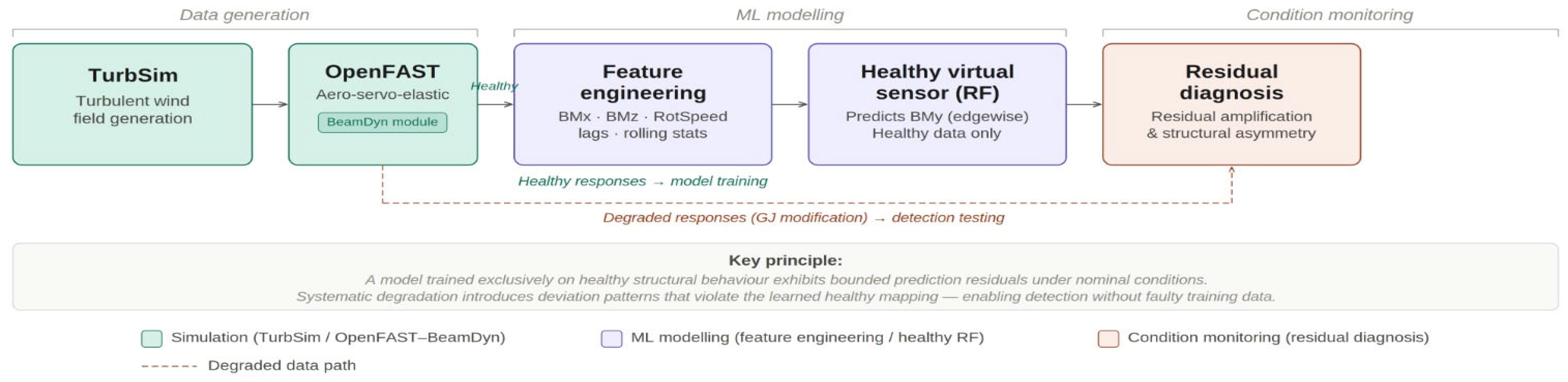
Simulation-driven virtual sensing framework. OpenFAST–BeamDyn aeroelastic simulations of the NREL 5 MW reference turbine generate blade-root moment responses under healthy and degraded conditions. A Random Forest virtual sensor is trained exclusively on healthy data using ten structural and kinematic features (solid teal path). Degraded responses—produced via controlled torsional stiffness (GJ) reduction—are passed to the trained model for residual-based fault detection (dashed coral path).
Figure 1.
Simulation-driven virtual sensing framework. OpenFAST–BeamDyn aeroelastic simulations of the NREL 5 MW reference turbine generate blade-root moment responses under healthy and degraded conditions. A Random Forest virtual sensor is trained exclusively on healthy data using ten structural and kinematic features (solid teal path). Degraded responses—produced via controlled torsional stiffness (GJ) reduction—are passed to the trained model for residual-based fault detection (dashed coral path).
Figure 2.
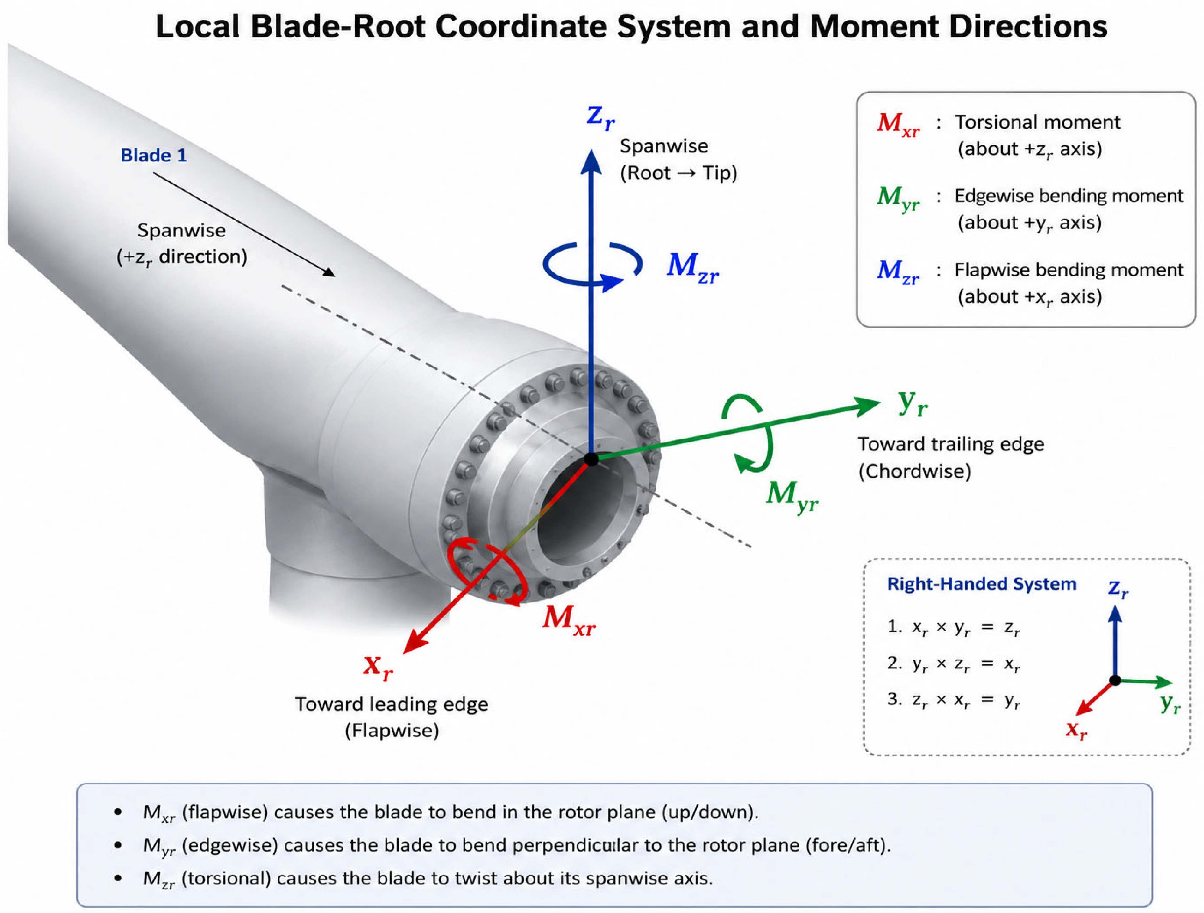
Local BeamDyn blade-root coordinate system and corresponding rotating-frame blade-root moment components used for structural virtual sensing; the dashed line indicates the blade spanwise axis (+z_r direction, root to tip).
Figure 2.
Local BeamDyn blade-root coordinate system and corresponding rotating-frame blade-root moment components used for structural virtual sensing; the dashed line indicates the blade spanwise axis (+z_r direction, root to tip).
Figure 3.
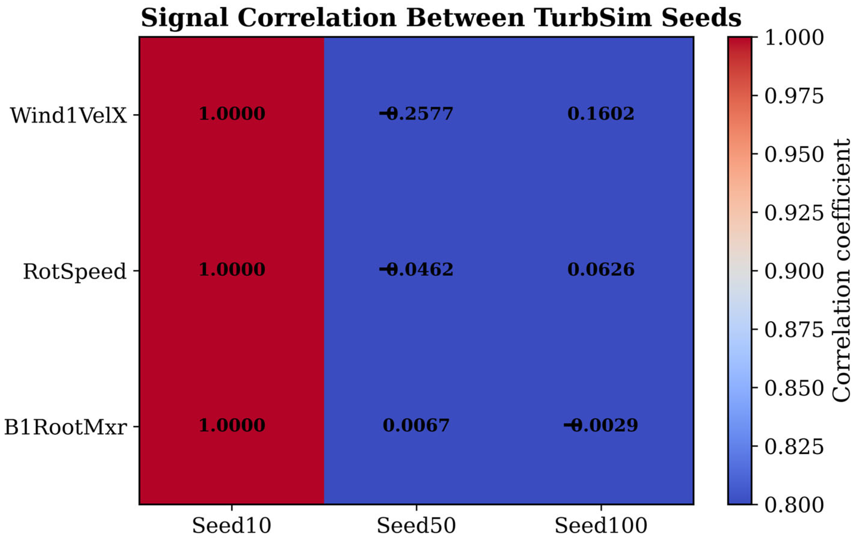
Cross-correlation analysis of representative TurbSim stochastic seeds used for healthy-condition dataset generation.
Figure 3.
Cross-correlation analysis of representative TurbSim stochastic seeds used for healthy-condition dataset generation.
Figure 4.
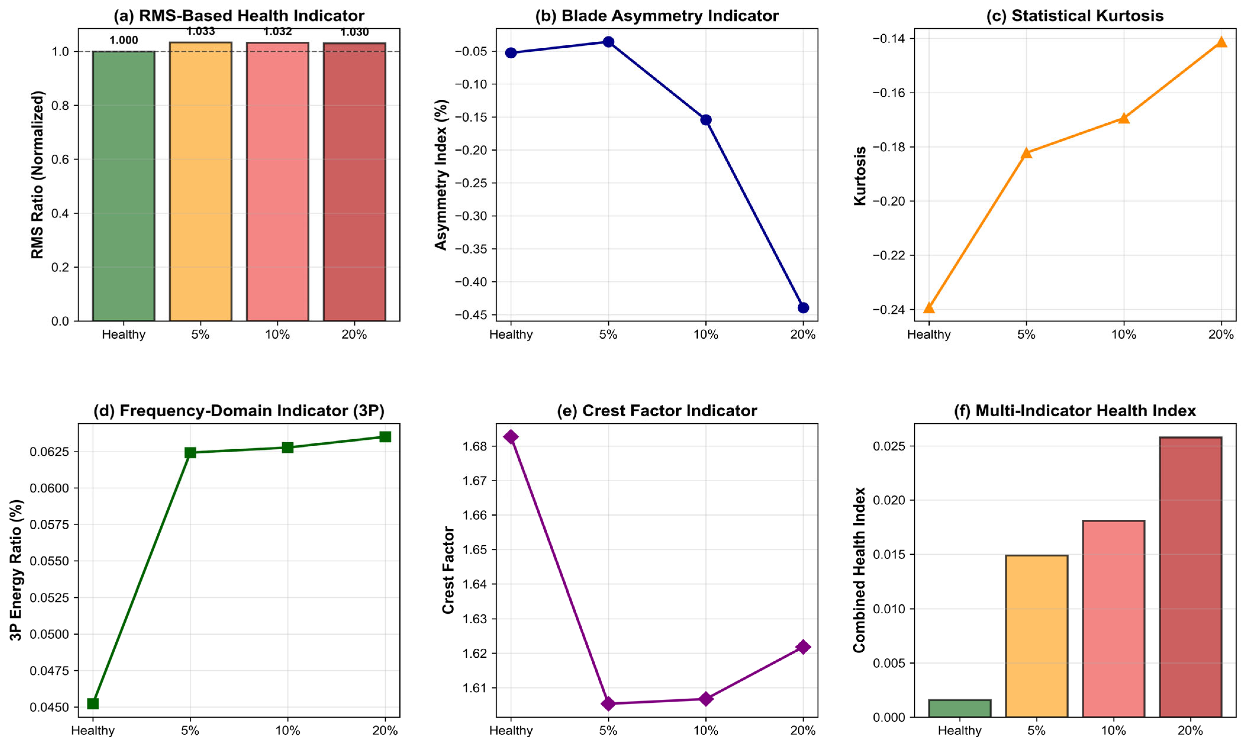
Multi-domain structural health indicators for healthy and faulty blade conditions under progressively decreasing torsional stiffness. (a) RMS-based health indicator, (b) blade asymmetry index, (c) statistical kurtosis, (d) frequency-domain 3P harmonic energy indicator, (e) crest factor indicator, and (f) combined multi-indicator health index evaluated for healthy, 5%, 10%, and 20% blade stiffness reduction cases generated using OpenFAST simulations. (The dashed horizontal line in panel (a) indicates the healthy-condition RMS baseline (normalised ratio = 1.000)).
Figure 4.
Multi-domain structural health indicators for healthy and faulty blade conditions under progressively decreasing torsional stiffness. (a) RMS-based health indicator, (b) blade asymmetry index, (c) statistical kurtosis, (d) frequency-domain 3P harmonic energy indicator, (e) crest factor indicator, and (f) combined multi-indicator health index evaluated for healthy, 5%, 10%, and 20% blade stiffness reduction cases generated using OpenFAST simulations. (The dashed horizontal line in panel (a) indicates the healthy-condition RMS baseline (normalised ratio = 1.000)).
Figure 5.
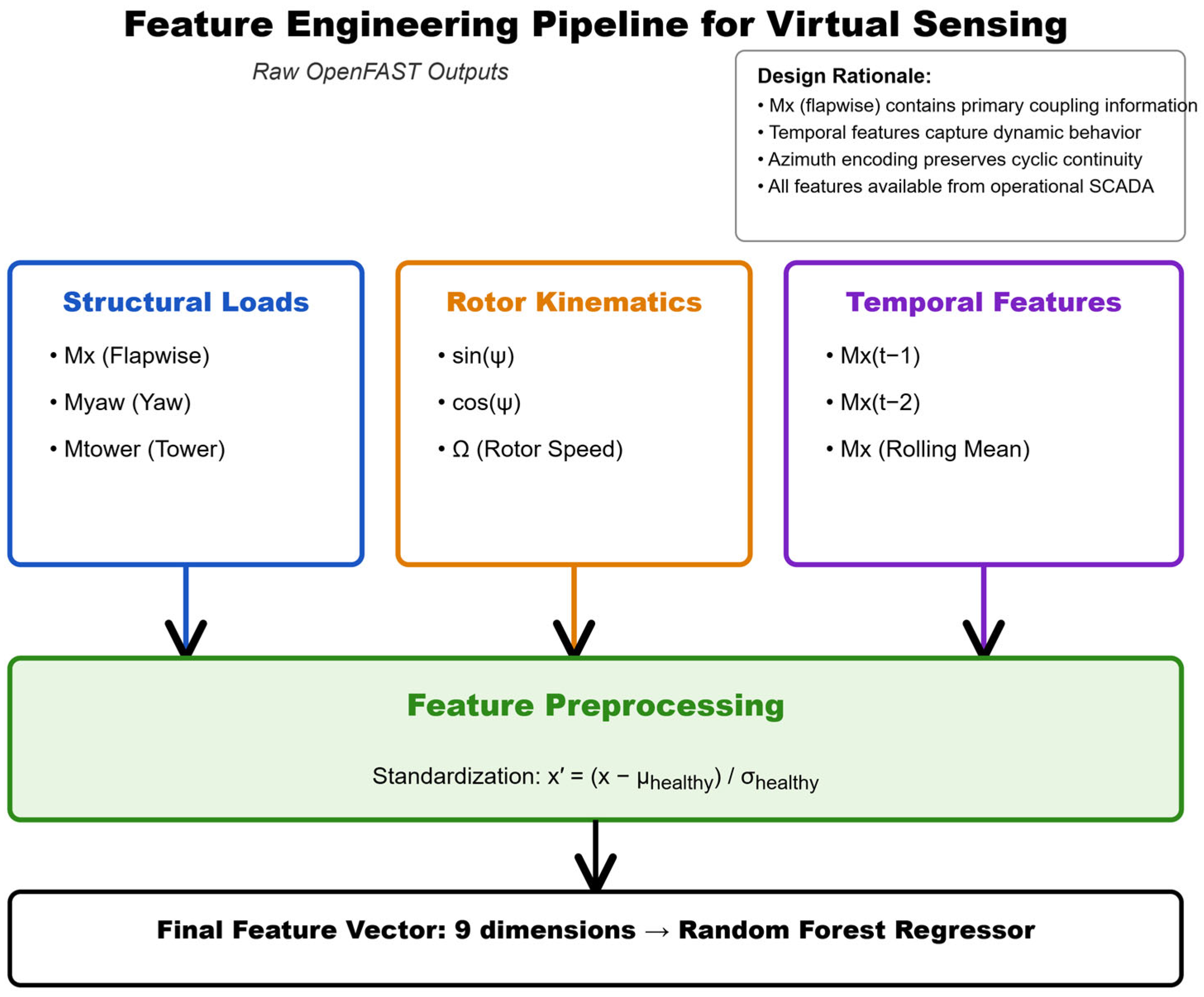
Structural feature-engineering pipeline adopted for the virtual sensing framework. Blue, orange, and purple boxes denote the structural load, rotor kinematic, and temporal feature groups, respectively. Coloured arrows indicate the flow of each feature group into the preprocessing stage, and the black arrow indicates the final assembled input vector passed to the Random Forest Regressor.
Figure 5.
Structural feature-engineering pipeline adopted for the virtual sensing framework. Blue, orange, and purple boxes denote the structural load, rotor kinematic, and temporal feature groups, respectively. Coloured arrows indicate the flow of each feature group into the preprocessing stage, and the black arrow indicates the final assembled input vector passed to the Random Forest Regressor.
Figure 6.
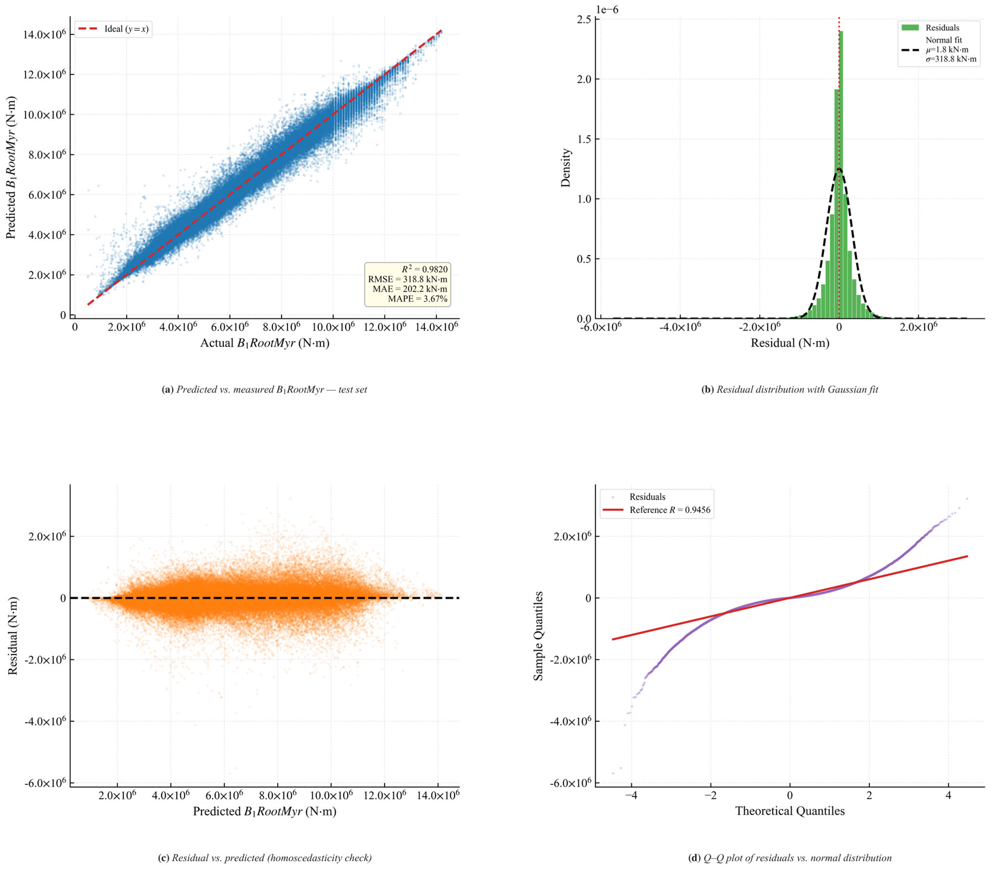
Virtual sensor diagnostic evaluation on the healthy test set. (a) Predicted versus measured B1RootMyr with perfect-agreement identity line (R2 = 0.9820, RMSE = 318,810 N·m, MAPE = 3.67%); (b) residual distribution with Gaussian fit centred at μ = 1800 N·m; (c) residual versus predicted load, homoscedasticity check; (d) Q-Q plot of standardised residuals (reference correlation R = 0.9456).
Figure 6.
Virtual sensor diagnostic evaluation on the healthy test set. (a) Predicted versus measured B1RootMyr with perfect-agreement identity line (R2 = 0.9820, RMSE = 318,810 N·m, MAPE = 3.67%); (b) residual distribution with Gaussian fit centred at μ = 1800 N·m; (c) residual versus predicted load, homoscedasticity check; (d) Q-Q plot of standardised residuals (reference correlation R = 0.9456).
Figure 7.
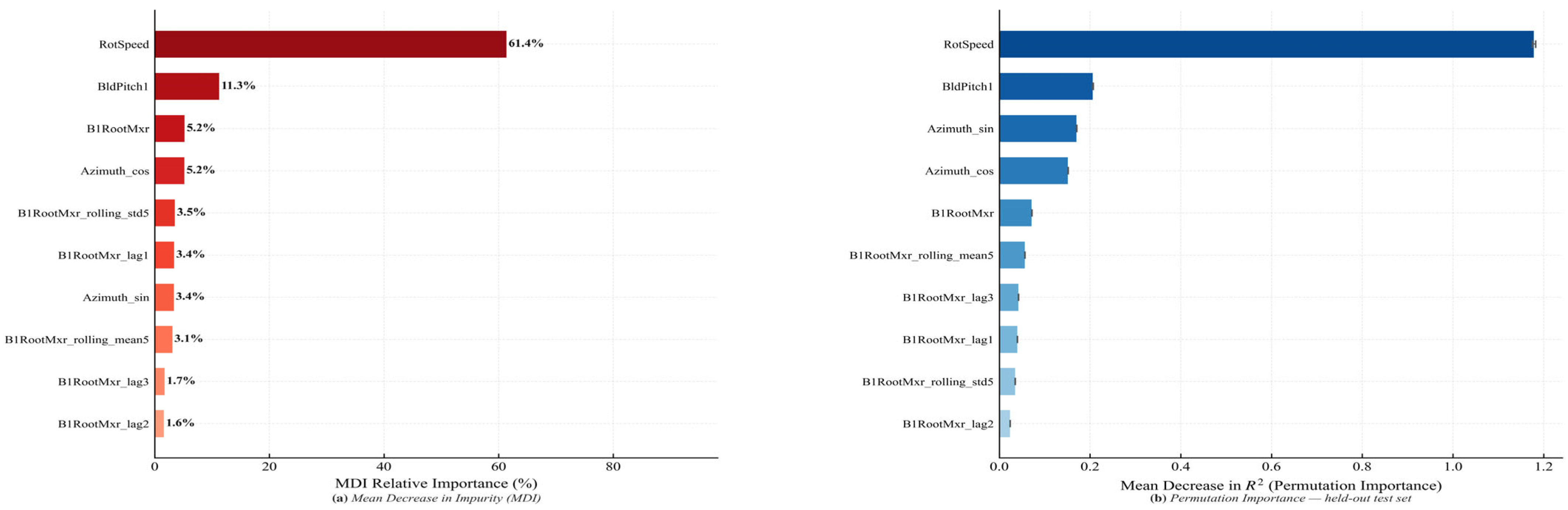
Feature importance analysis for the Random Forest virtual sensor. (a) MDI from the training ensemble (dark to light red = highest to lowest importance); (b) permutation importance (mean ΔR2) on the held-out test set (dark to light blue = highest to lowest). Both methods confirm consistent, physically meaningful feature rankings.
Figure 7.
Feature importance analysis for the Random Forest virtual sensor. (a) MDI from the training ensemble (dark to light red = highest to lowest importance); (b) permutation importance (mean ΔR2) on the held-out test set (dark to light blue = highest to lowest). Both methods confirm consistent, physically meaningful feature rankings.
Figure 8.
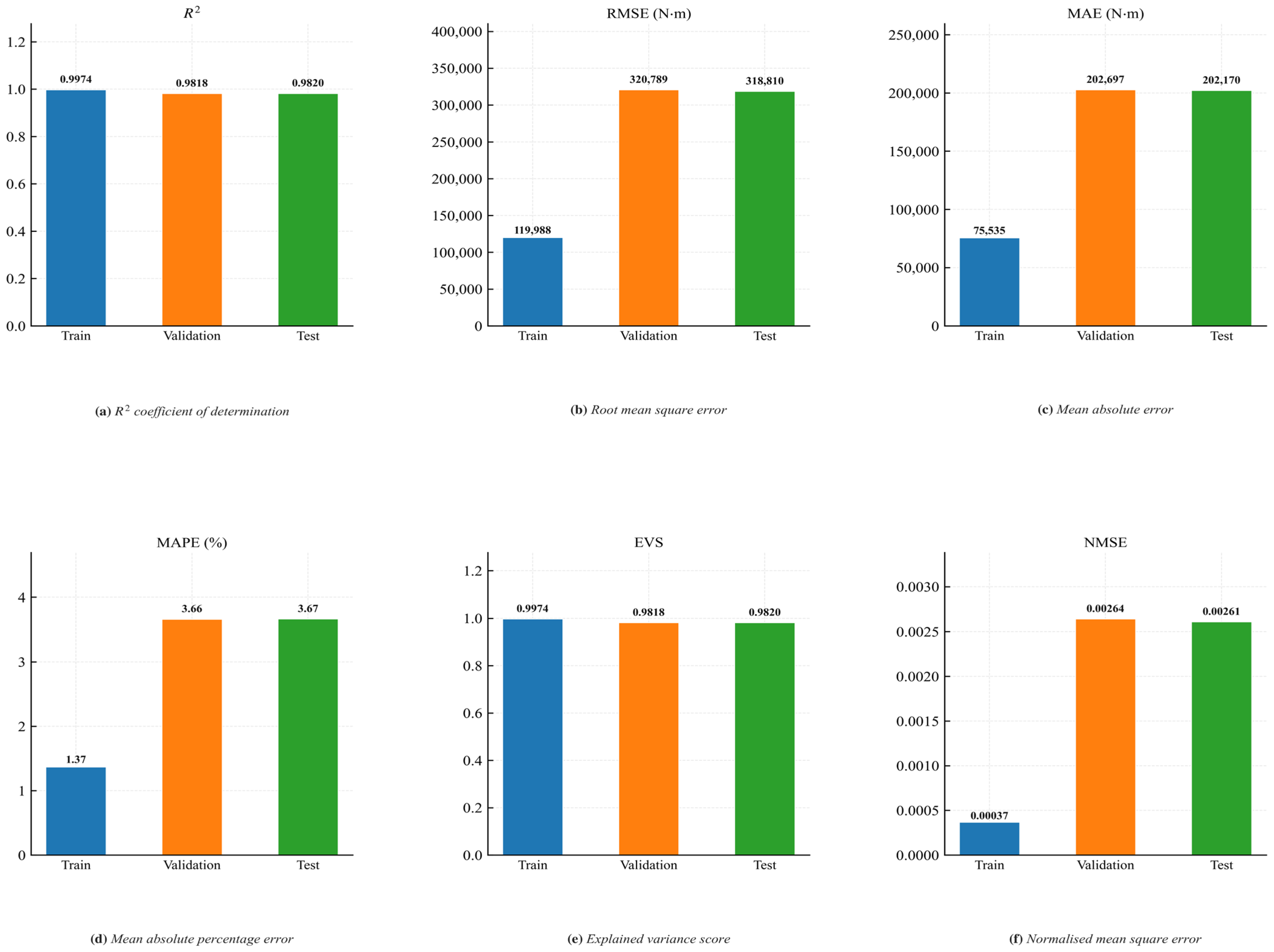
Random Forest virtual sensing model performance metrics across train (blue), validation (orange), and test (green) data partitions. Six panels show (a) R2, (b) RMSE (N·m), (c) MAE (N·m), (d) MAPE (%), (e) Explained Variance Score (EVS), and (f) Normalised Mean Squared Error (NMSE).
Figure 8.
Random Forest virtual sensing model performance metrics across train (blue), validation (orange), and test (green) data partitions. Six panels show (a) R2, (b) RMSE (N·m), (c) MAE (N·m), (d) MAPE (%), (e) Explained Variance Score (EVS), and (f) Normalised Mean Squared Error (NMSE).
Figure 9.
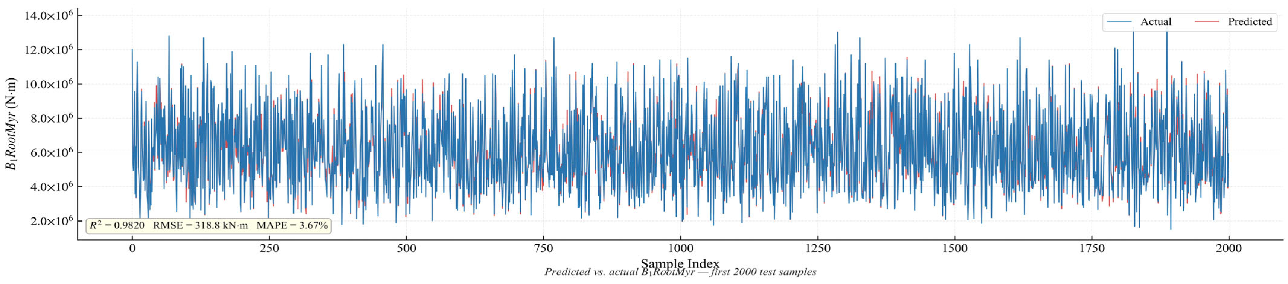
Time-series tracking performance over the first 2000 unseen test samples. Actual B1RootMyr (blue) and predicted B1RootMyr (red) are overlaid, demonstrating accurate reproduction of high-frequency aeroelastic load fluctuations (R2 = 0.9820, RMSE = 318,810 N·m, MAPE = 3.67%).
Figure 9.
Time-series tracking performance over the first 2000 unseen test samples. Actual B1RootMyr (blue) and predicted B1RootMyr (red) are overlaid, demonstrating accurate reproduction of high-frequency aeroelastic load fluctuations (R2 = 0.9820, RMSE = 318,810 N·m, MAPE = 3.67%).
Figure 10.
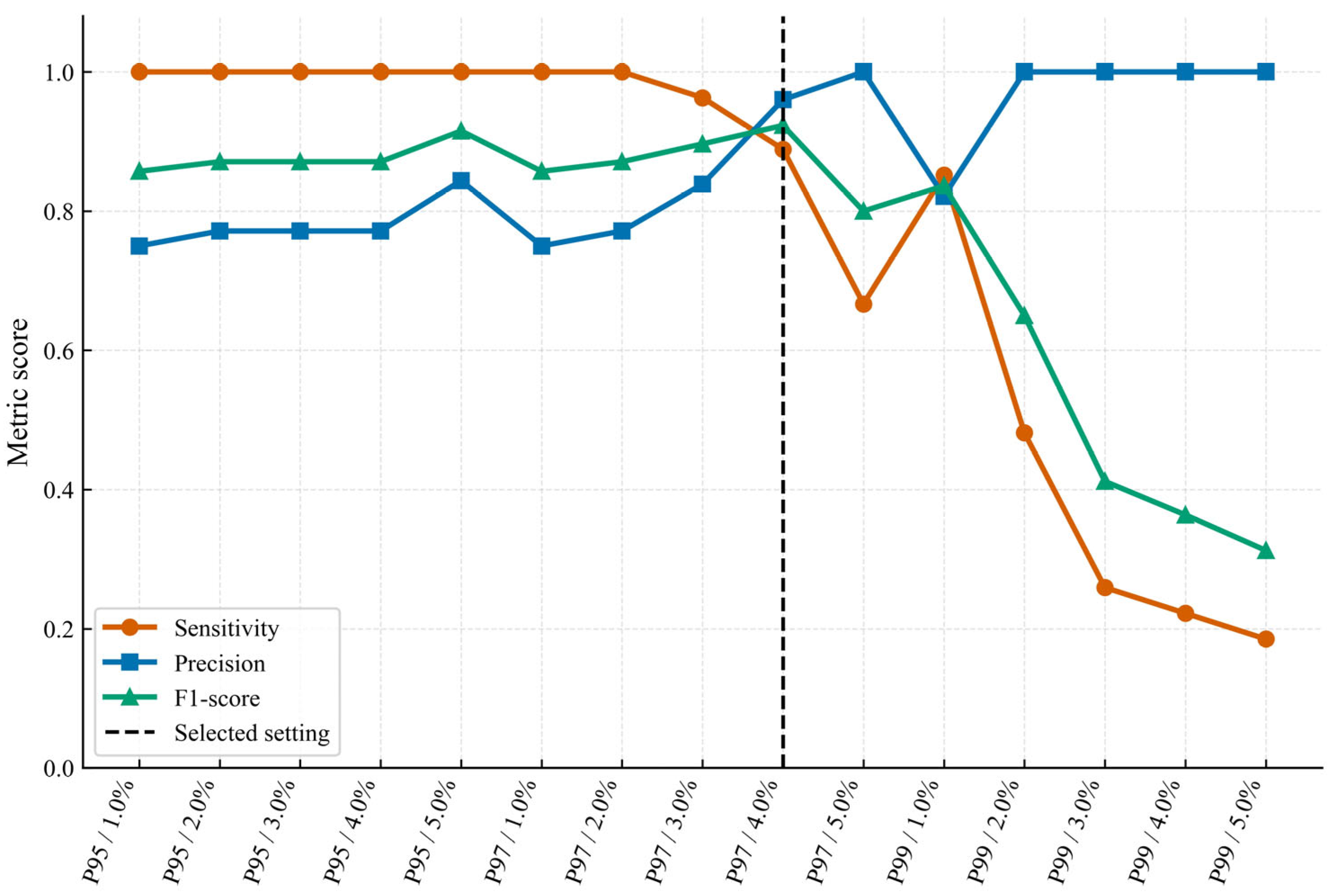
Threshold grid-search sensitivity analysis. Sensitivity (orange circles), precision (blue squares), and F1-score (green triangles) across all 15 parameter combinations (P95–P99 × 1–5%). The vertical dashed line indicates the selected operating point, P97/4.0%, which achieves the highest F1-score (0.923) among all settings with precision ≥ 0.90.
Figure 10.
Threshold grid-search sensitivity analysis. Sensitivity (orange circles), precision (blue squares), and F1-score (green triangles) across all 15 parameter combinations (P95–P99 × 1–5%). The vertical dashed line indicates the selected operating point, P97/4.0%, which achieves the highest F1-score (0.923) among all settings with precision ≥ 0.90.
Figure 11.
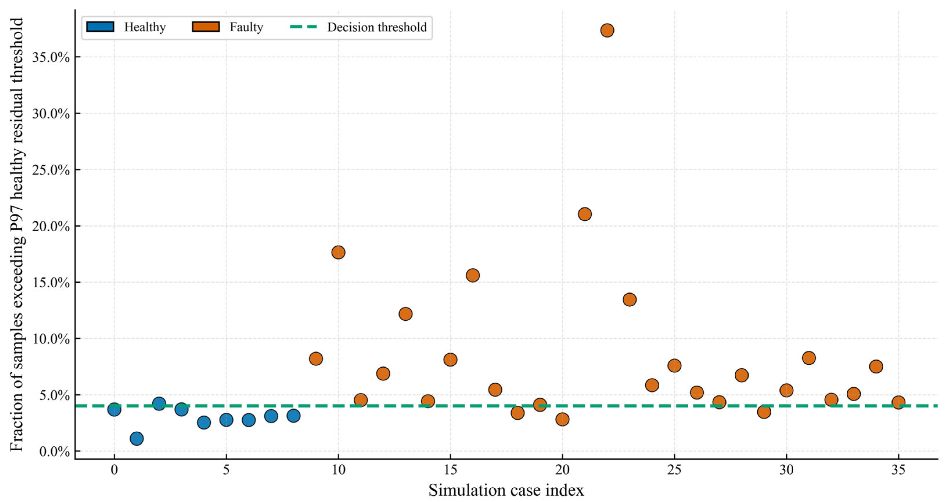
Case-level residual exceedance fractions (f_ws) for all 36 test cases plotted against simulation case index. Healthy cases (blue) cluster below the 4.0% decision threshold; faulty cases (orange) exhibit progressive exceedance amplification with increasing torsional stiffness reduction severity. The dashed green line indicates the selected decision boundary.
Figure 11.
Case-level residual exceedance fractions (f_ws) for all 36 test cases plotted against simulation case index. Healthy cases (blue) cluster below the 4.0% decision threshold; faulty cases (orange) exhibit progressive exceedance amplification with increasing torsional stiffness reduction severity. The dashed green line indicates the selected decision boundary.
Figure 12.
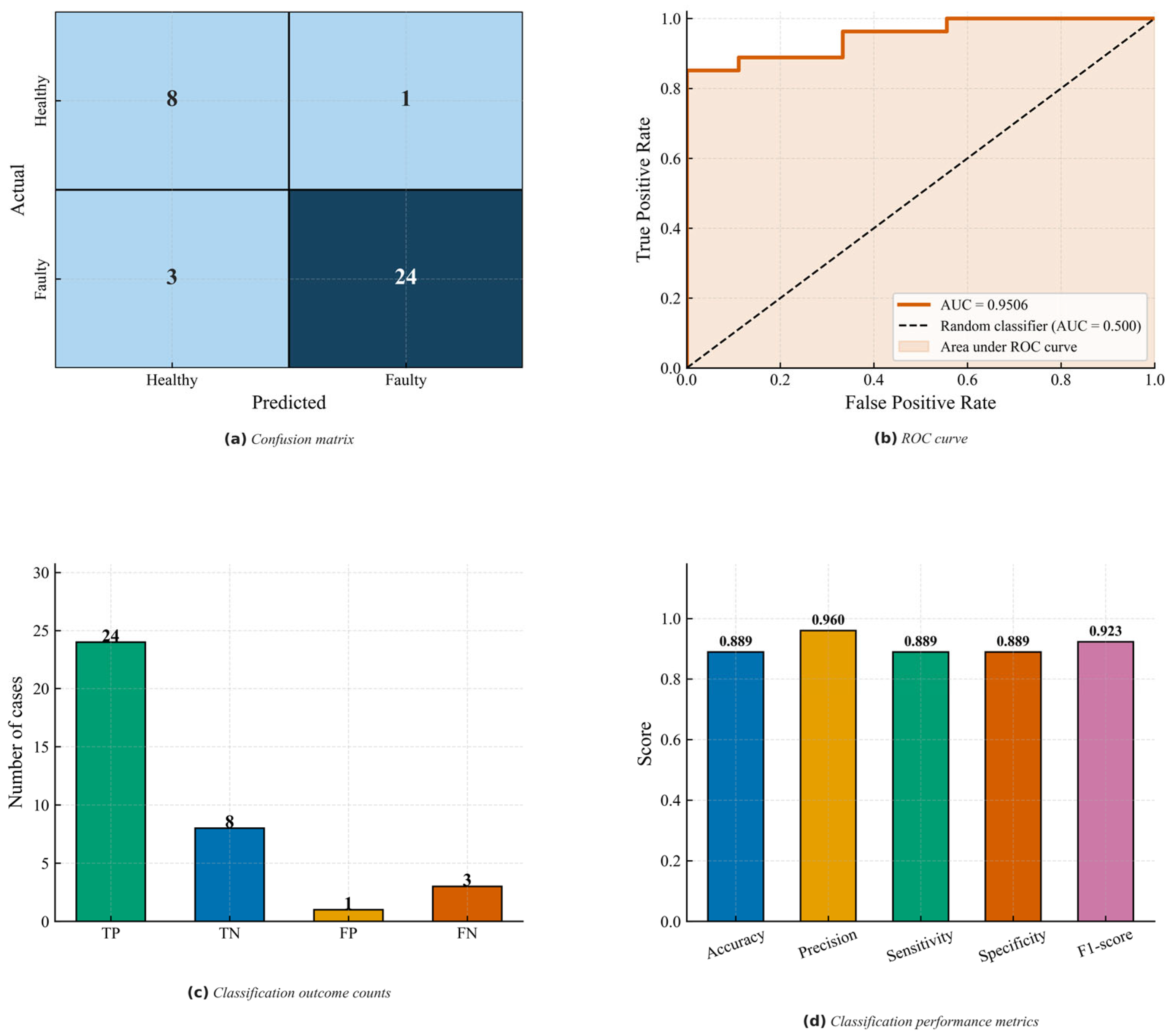
Fault classification results at the P97/4.0% operating point. (a) Confusion matrix (TP = 24, TN = 8, FP = 1, FN = 3); (b) ROC curve (AUC = 0.951), where the dashed diagonal line represents the random classifier baseline (AUC = 0.500) and the shaded region indicates the area under the ROC curve; (c) classification outcome counts; (d) performance metrics bar chart.
Figure 12.
Fault classification results at the P97/4.0% operating point. (a) Confusion matrix (TP = 24, TN = 8, FP = 1, FN = 3); (b) ROC curve (AUC = 0.951), where the dashed diagonal line represents the random classifier baseline (AUC = 0.500) and the shaded region indicates the area under the ROC curve; (c) classification outcome counts; (d) performance metrics bar chart.
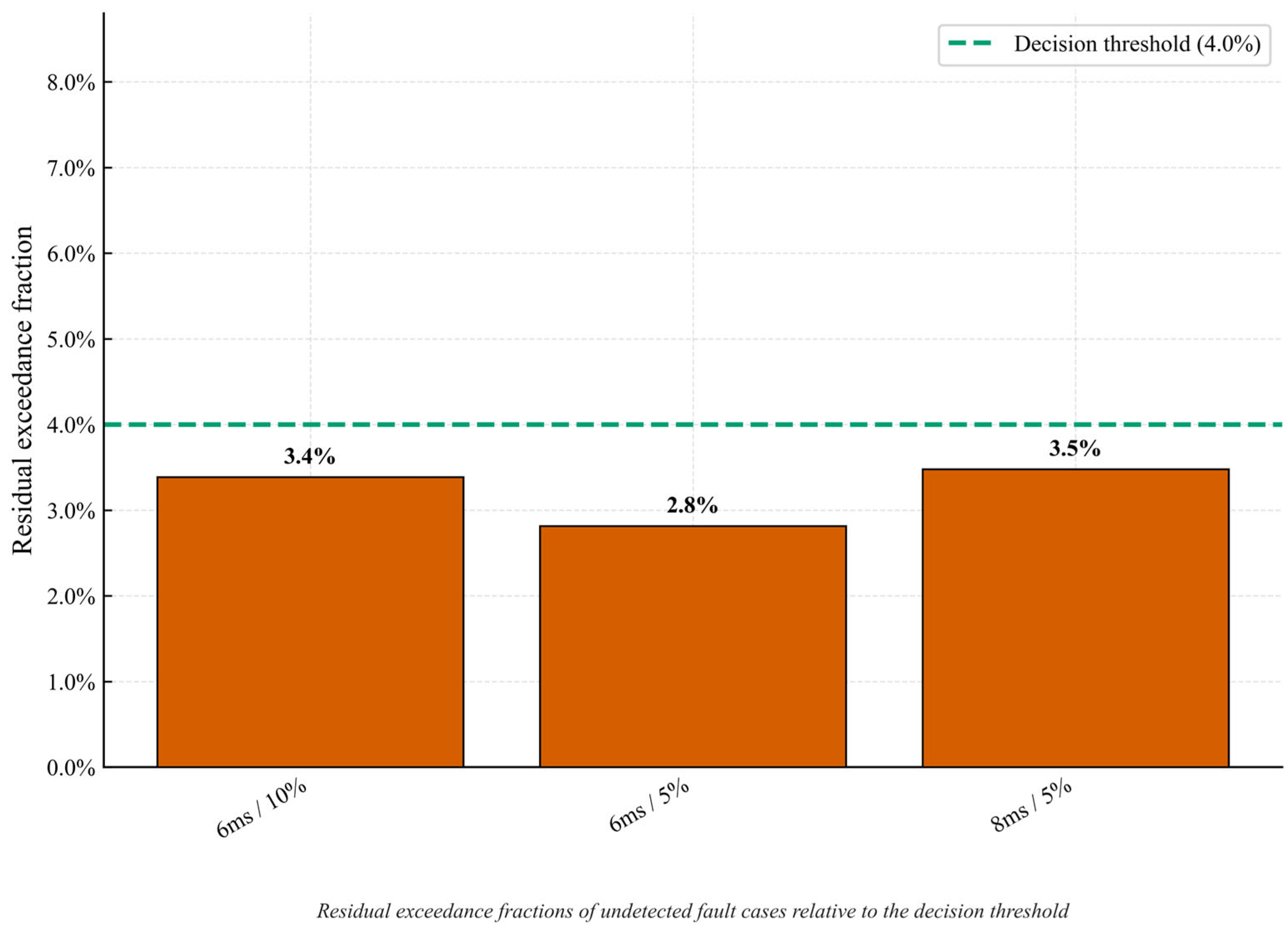
Figure 13.
Residual exceedance fractions of the three undetected (false-negative) fault cases relative to the 4.0% decision threshold (green dashed line). All three cases fall below the threshold, with exceedance fractions between 2.8% and 3.5%, indicating marginal separation from the healthy decision boundary.
Figure 13.
Residual exceedance fractions of the three undetected (false-negative) fault cases relative to the 4.0% decision threshold (green dashed line). All three cases fall below the threshold, with exceedance fractions between 2.8% and 3.5%, indicating marginal separation from the healthy decision boundary.
Table 1.
Summary of OpenFAST healthy and faulty simulation datasets.
Table 1.
Summary of OpenFAST healthy and faulty simulation datasets.
| Dataset | Wind Speeds | TurbSim Seed IDs | Cases | Simulation Time | Effective Time After 30 s Removal | Purpose |
|---|
| Healthy | 6, 8, 12 m/s | 10, 50, 100 | 9 | 600 s | 570 s | RFR training, validation, testing, threshold baseline |
| Faulty | 6, 8, 12 m/s | 10, 50, 100 | 27 | 200 s | 170 s | Independent fault evaluation |
| Fault severities | 5%, 10%, 20% GJ reduction | — | 27 | 200 s | 170 s | Blade 1 torsional degradation testing |
Table 2.
Engineered structural-response features used for Random Forest virtual sensing.
Table 2.
Engineered structural-response features used for Random Forest virtual sensing.
| Feature | Category | Physical Interpretation |
|---|
| RotSpeed | Rotor kinematics | Inertia-driven edgewise loading component |
| BldPitch1 | Aerodynamic ctrl | Blade pitch angle aerodynamic load control |
| B1RootMxr | Structural load | Blade 1 flapwise blade-root bending response |
| B1RootMxr_lag1 | Temporal feature | One-step historical flapwise load memory |
| B1RootMxr_lag2 | Temporal feature | Two-step historical flapwise load memory |
| B1RootMxr_lag3 | Temporal feature | Three-step historical flapwise load memory |
| Azimuth_ | Cyclic feature | Rotor azimuth periodicity encoding(sin) |
| Azimuth_ | Cyclic feature | Rotor azimuth periodicity encoding(cos) |
| B1RootMxr_rolling_mean5 | Rolling statistical feature | 5-sample rolling mean-local trend |
| B1RootMxr_rolling_std5 | Rolling statistical feature | 5-sample rolling std-local trend |
Table 3.
Random Forest virtual sensing model configuration.
Table 3.
Random Forest virtual sensing model configuration.
| Parameter | Final Configuration |
|---|
| Model Specification |
| Algorithm | Random Forest Regressor (scikit-learn v1.4.0 (INRIA, Paris, France)) |
| Prediction target | B1RootMyr (edgewise blade-root moment, N·m) |
| Number of input features | 10 (see Table 2) |
| Training data | Healthy-condition simulations only |
| Wind speed conditions | 6 m/s, 8 m/s, 12 m/s |
| Data Partitioning |
| Split strategy | Stratified random split by wind speed |
| Train/validation/test | 60%/20%/20% |
| Stratification variable | Wind speed bin (balanced coverage across regimes) |
| Hyperparameter Optimisation |
| Search algorithm | RandomizedSearchCV |
| Cross-validation | 3-fold |
| Candidate evaluations | 25 |
| Scoring criterion | R2 (coefficient of determination) |
| Optimised Hyperparameters |
| n_estimators | 500 |
| max_depth | None (fully grown trees, no pruning) |
| min_samples_split | 2 |
| min_samples_leaf | 1 |
| max_features | 0.4 |
| Bootstrap | True (sampling with replacement) |
| oob_score | Enabled (out-of-bag generalisation estimate) |
| Reproducibility and Performance |
| Random seed | 42 |
| Feature importance method | Mean Decrease in Impurity (MDI) and permutation importance |
| Training time (CPU) | 45.3 min |
| Inference speed | <1 ms per sample (real-time capable) |
Table 4.
Prediction performance of the Random Forest virtual sensor on the healthy test dataset.
Table 4.
Prediction performance of the Random Forest virtual sensor on the healthy test dataset.
| Metric | Value |
|---|
| R2 | 0.9820 |
| RMSE (N·m) | 318,810 |
| MAE (N·m) | 202,170 |
| MAPE (%) | 3.67 |
| EVS | 0.9820 |
| NMSE | 0.00261 |
Table 5.
Feature importance rankings by MDI and permutation importance on the test set.
Table 5.
Feature importance rankings by MDI and permutation importance on the test set.
| Feature | MDI (%) | Perm. ΔR2 | Perm. SD |
|---|
| RotSpeed | 61.4 | 1.179 | 0.0036 |
| BldPitch1 | 11.3 | 0.206 | 0.0009 |
| B1RootMxr | 5.2 | 0.072 | 0.0002 |
| Azimuth_cos | 5.2 | 0.152 | 0.0004 |
| B1RootMxr_rolling_std5 | 3.5 | 0.035 | 0.0001 |
| B1RootMxr_lag1 | 3.4 | 0.040 | 0.0001 |
| Azimuth_sin | 3.4 | 0.171 | 0.0004 |
| B1RootMxr_rolling_mean5 | 3.1 | 0.057 | 0.0002 |
| B1RootMxr_lag3 | 1.7 | 0.042 | 0.0002 |
| B1RootMxr_lag2 | 1.6 | 0.024 | 0.0001 |
Table 6.
Generalisation performance of the Random Forest virtual sensor across data partitions.
Table 6.
Generalisation performance of the Random Forest virtual sensor across data partitions.
| Dataset | R2 | RMSE (N·m) | MAE (N·m) | MAPE (%) |
|---|
| Training | 0.9974 | 119,988 | 75,535 | 1.37 |
| Validation | 0.9818 | 320,789 | 202,697 | 3.66 |
| Test | 0.9820 | 318,810 | 202,170 | 3.67 |
Table 7.
Wind-speed-specific P97 residual thresholds derived from pooled healthy test-case residuals (N = 273,600 samples per wind speed).
Table 7.
Wind-speed-specific P97 residual thresholds derived from pooled healthy test-case residuals (N = 273,600 samples per wind speed).
| Wind Speed | N Samples | Mean |Residual| (N·m) | P97 Threshold τ (N·m) |
|---|
| 6 m/s | 273,600 | 88,579 | 407,981 |
| 8 m/s | 273,600 | 130,897 | 552,881 |
| 12 m/s | 273,600 | 151,330 | 734,264 |
Table 8.
Threshold grid-search results across all 15 parameter combinations.
Table 8.
Threshold grid-search results across all 15 parameter combinations.
| Setting | TP | TN | FP | FN | Acc. | Prec. | Sens. | Spec. | F1 |
|---|
| P95/1% | 27 | 0 | 9 | 0 | 0.750 | 0.750 | 1.000 | 0.000 | 0.857 |
| P95/2% | 27 | 1 | 8 | 0 | 0.778 | 0.771 | 1.000 | 0.111 | 0.871 |
| P95/3% | 27 | 1 | 8 | 0 | 0.778 | 0.771 | 1.000 | 0.111 | 0.871 |
| P95/4% | 27 | 1 | 8 | 0 | 0.778 | 0.771 | 1.000 | 0.111 | 0.871 |
| P95/5% | 27 | 4 | 5 | 0 | 0.861 | 0.844 | 1.000 | 0.444 | 0.915 |
| P97/1% | 27 | 0 | 9 | 0 | 0.750 | 0.750 | 1.000 | 0.000 | 0.857 |
| P97/2% | 27 | 1 | 8 | 0 | 0.778 | 0.771 | 1.000 | 0.111 | 0.871 |
| P97/3% | 26 | 4 | 5 | 1 | 0.833 | 0.839 | 0.963 | 0.444 | 0.897 |
| 1 P97/4% | 24 | 8 | 1 | 3 | 0.889 | 0.960 | 0.889 | 0.889 | 0.923 |
| P97/5% | 18 | 9 | 0 | 9 | 0.750 | 1.000 | 0.667 | 1.000 | 0.800 |
| P99/1% | 23 | 4 | 5 | 4 | 0.750 | 0.821 | 0.852 | 0.444 | 0.836 |
| P99/2% | 13 | 9 | 0 | 14 | 0.611 | 1.000 | 0.481 | 1.000 | 0.650 |
| P99/3% | 7 | 9 | 0 | 20 | 0.444 | 1.000 | 0.259 | 1.000 | 0.412 |
| P99/4% | 6 | 9 | 0 | 21 | 0.417 | 1.000 | 0.222 | 1.000 | 0.364 |
| P99/5% | 5 | 9 | 0 | 22 | 0.389 | 1.000 | 0.185 | 1.000 | 0.312 |
Table 9.
Fault detection performance by wind speed.
Table 9.
Fault detection performance by wind speed.
| Wind Speed | Detected | Missed | Total | Detection Rate (%) |
|---|
| 6 m/s | 7 | 2 | 9 | 77.8 |
| 8 m/s | 8 | 1 | 9 | 88.9 |
| 12 m/s | 9 | 0 | 9 | 100.0 |
| Overall | 24 | 3 | 27 | 88.9 |
Table 10.
Confusion matrix at the P97/4.0% operating point.
Table 10.
Confusion matrix at the P97/4.0% operating point.
| | Predicted Healthy | Predicted Faulty |
|---|
| Healthy | TN = 8 | FP = 1 |
| Faulty | FN = 3 | TP = 24 |
Table 11.
Fault classification performance at the selected P97/4.0% operating point.
Table 11.
Fault classification performance at the selected P97/4.0% operating point.
| Metric | Value |
|---|
| Accuracy | 0.889 |
| Precision | 0.960 |
| Sensitivity (Recall) | 0.889 |
| Specificity | 0.889 |
| F1-score | 0.923 |
| AUC–ROC | 0.951 |
Table 12.
Fault detection rates stratified by degradation severity level (3 seeds × 3 wind speeds = 9 cases per severity level; P97/4.0% threshold).
Table 12.
Fault detection rates stratified by degradation severity level (3 seeds × 3 wind speeds = 9 cases per severity level; P97/4.0% threshold).
| Severity | Detected | Missed | Total | Detection Rate |
|---|
| 5% GJ reduction | 7 | 2 | 9 | 77.8% |
| 10% GJ reduction | 8 | 1 | 9 | 88.9% |
| 20% GJ reduction | 9 | 0 | 9 | 100.0% |
| Overall | 24 | 3 | 27 | 88.9% |
Table 13.
Undetected (false-negative) fault cases at the P97/4.0% operating point.
Table 13.
Undetected (false-negative) fault cases at the P97/4.0% operating point.
| Case (Abbreviated) | Wind Speed | GJ Reduction | RMSE (N·m) | Exceedance f_ws |
|---|
| 5MW…6m/s_100_10pct | 6m/s | 10% | 162,236 | 3.4% |
| 5MW…6m/s_100_5pct | 6m/s | 5% | 152,823 | 2.8% |
| 5MW…8m/s_100_5pct | 8m/s | 5% | 223,629 | 3.5% |
Table 14.
Comparison between case-level RMSE thresholding and sample-level residual exceedance classification.
Table 14.
Comparison between case-level RMSE thresholding and sample-level residual exceedance classification.
| Method | TP | TN | FP | FN | Accuracy | Precision | Sensitivity | F1-Score | AUC |
|---|
| RMSE Threshold | 17 | 9 | 0 | 10 | 0.722 | 1.000 | 0.630 | 0.773 | 0.774 |
| Residual Exceedance | 24 | 8 | 1 | 3 | 0.889 | 0.960 | 0.889 | 0.923 | 0.951 |