L21RSVD: Robust L21 Norm SVD-Type Latent Factor Models for Rating Prediction

Abstract

Recommender systems face fundamental challenges, including extreme data sparsity and noisy rating observations. We propose L21RSVD, a robust latent factor model that employs L21 norm regularization within a Singular Value Decomposition framework to mitigate the impact of outliers while preserving low-rank structure. Unlike conventional L2-regularized approaches, our formulation induces group sparsity in the latent factor space, yielding more discriminative user and item representations. We derive three optimization variants: standard L21RSVD, L21RSVD without the squared term, and coefficient-free adaptive L21RSVD. Building upon these, we introduce a fusion strategy that adaptively aggregates predictions based on local data density. Extensive experiments on benchmark datasets demonstrate that L21RSVD substantially outperforms classical collaborative filtering and the SVD-type model. The proposed fusion model achieves state-of-the-art performance, reducing RMSE by up to 31.21% and MAE by up to 42.99% relative to baseline methods.

1. Introduction

With the further development of information technology and big data, there is a serious overload of information nowadays, and RSs (recommender systems) [1], as the core technology to solve the information overload and achieve personalized services, have been widely used in e-commerce, social media, movie recommendation [2,3,4] and other entertainment industries in recent years under the impetus of big data and machine learning. In most practical applications of recommender systems, users can rate each item at multiple levels, ranging from 1.0 (least interested) to 5.0 (most interested). In general, the number of ratings from users for items is very limited, which results in a very sparse dataset. The task of the recommender system is to predict each user’s rating of an item that has not yet been rated by analyzing the entire existence of rating data. Collaborative Filter [5,6,7] is one of the key algorithms in the recommendation system area. There are many patterns in user behavior in recommender systems; the main idea of user behavior-based recommendation is to use the historical behavioral data of existing users (explicit or implicit feedback) to predict the items that the current user may be interested in, of which the explicit feedback is mainly user ratings, and the implicit feedback mainly includes browsing, searching, and so on [8,9]. However, the significant defects of this algorithm are usually data sparsity; the user–item matrix is usually highly sparse, resulting in inaccurate similarity calculation and reduced recommendation quality.

The SVD [10,11,12] (Singular Value Decomposition) is a useful algorithm of dimensionality reduction. However, the limitations of this algorithm are: in terms of computational overhead, SVD needs to decompose the complete matrix, and the computational efficiency decreases when the rating matrix is extremely sparse; in terms of linear assumptions, the hidden factor model only captures linear relationships, which makes it difficult to model complex interactions, and in terms of the cold-start problem: the lack of ratings of new users/items does not enable the generation of the hidden vectors, which need to be combined with the contents or social information. Regularized Singular Value Decomposition is a matrix decomposition method that introduces regularization terms on top of the traditional Singular Value Decomposition. It is mainly used to deal with problems such as user–item rating matrices in areas such as recommender systems. While traditional SVD decomposes the original matrix into a product of three matrices, revealing underlying patterns and structures, Regularized SVD [13,14] prevents overfitting by adding a regularization term. This regularization term is usually a constraint on the underlying feature vectors of users and items, such as L2 regularization, which allows the model to fit the data without being overly reliant on specific training data points, thus improving the model’s ability to generalize on new data. However, Regularized SVD also has some weaknesses. On the computational side, its computational complexity is high, especially for large-scale matrices, and the decomposition and optimization process require a great deal of computational resources and time. Moreover, it has a limited ability to handle sparse data, and when the data is extremely sparse, it is difficult for the model to accurately estimate the potential features. It is also sensitive to noise in the data and cannot effectively distinguish between noise and useful information. In terms of model parameter selection, it is more difficult to determine the regularization parameters, which need to be adjusted through a large number of experiments, and may lead to overfitting or underfitting if not properly selected. In addition, it cannot make full use of the structural information of the original data, such as the complex structure of the social network relationship between users and items.

While traditional Regularized SVD (RSVD) employs the $L_2$ norm which is sensitive to outliers and rating noise, and while simple $L_1$ norm regularization lacks the ability to capture group sparsity, our work introduces the $L_{2,1}$ norm into the SVD framework. Unlike the $L_1$ norm that induces element-wise sparsity, the $L_{2,1}$ norm induces row-wise sparsity in the latent factor space. This is a key distinction: it allows the model to automatically identify and suppress unimportant users or items as a whole (group sparsity), rather than just shrinking individual weights. To the best of our knowledge, this is the first work that systematically applies the $L_{2,1}$-norm regularization within a fusion SVD framework for rating prediction.

In view of the above shortcomings of the recommendation system algorithm, we develop a L21RSVD fusion model, which includes three L21RSVD models for rating prediction in recommending systems. Based on the error generated by the SVD model, the L21 norm [15,16,17] is used to replace the L2 norm in the scoring matrix, and the related loss function is established and optimized. The main contributions of this paper are summarized as follows:

(1)

We introduce the L21 norm into recommendation systems to address the challenge of data sparsity within such systems.

(2)

To comprehensively demonstrate the characteristics of L21RSVD, three variants of the L21RSVD model are proposed.

(3)

Subsequently, based on these three variants as baseline models, we develop an L21RSVD fusion model, which improves the robustness and universality of the recommender system algorithm.

(4)

Compared to SOTA recommendation system algorithms, the L21RSVD fusion model reduces RMSE by up to 31.21% and MAE by up to 42.99%.

(5)

Experimental results on real-world datasets demonstrate that our L21RSVD fusion approach outperforms other benchmark methods in terms of root mean square error and mean absolute error, and more effectively addresses correlation issues.

The main structure of this paper is organized as follows: Section 2 is the analysis of related work; Section 3 introduces three variants of the L21RSVD algorithm and subsequently proposes the L21RSVD fusion model based on these three methods; Section 4 is the experimental validation and analysis; and Section 5 concludes this paper with a conclusion and future work.

2. Related Work

2.1. Collaborative Filter Algorithm

The Collaborative Filter recommendation algorithm is one of the key technologies in the artificial intelligence (AI) area. The concept of recommender systems was first formally introduced by Resnick [18]. At this time, the recommender system actually refers to collaborative filtering. Collaborative filtering is one of the earliest proposed, but also the most researched and most practically applied recommendation techniques [19]. For the classification of collaborative filtering algorithms, there are two main classifications. The literature [20,21] classifies collaborative filtering algorithms into non-probabilistic and probabilistic algorithms by considering whether the algorithms are based on a basic probabilistic model. The literature [6,7] classifies algorithms into Memory-Based Collaborative Filtering algorithms and model-based collaborative filtering. There are many patterns in user behavior in recommender systems; for example, the famous case of “beer and nappies” [22] is a good example of user behavior patterns. The main idea of user behavior-based recommendation is to use the historical behavioral data of existing users (explicit or implicit feedback) to predict the items that the current user may be interested in, where the explicit feedback is mainly user ratings, and the implicit feedback mainly includes browsing, searching, and so on. Recommendation algorithms based on user behavior, also known as Collaborative Filtering Recommendation, which is the most widely used algorithm in the field of recommendation, do not need to obtain the characteristics of the user or the item in advance, and rely only on the user’s history of behavioral data to model the user, so as to recommend for the user. Collaborative filtering algorithms mainly include User-Based collaborative filtering (User-Based CF), Item-Based collaborative filtering (Item-Based CF), and so on. Among them, User-Based and Item-Based collaborative filtering analyses the data through statistical methods, so it is also called Memory-Based Collaborative Filtering or Neighborhood-Based Collaborative Filtering, which derives a model by learning the data, and then makes predictions and recommendations based on the model.

2.1.1. User-Based Collaborative Filtering Algorithm

The basic idea of a User-Based collaborative filtering algorithm [20,23] is to recommend items to a user that are of interest to users with similar interests to him or her. When a recommendation is needed for user A, first, find the set of users (denoted by U) with similar interests to A, and then, recommend the items in set U that are of interest to the user but have not been heard of by A. The algorithm is divided into two steps: first, the similarity between users is calculated, and the most similar of the N users is selected; then, the user ratings are calculated based on the similarity. Finally, the item with high similarity is recommended to the user. However, the significant defects of this algorithm are usually data sparsity: the user–item matrix is usually highly sparse, resulting in inaccurate similarity calculation and reduced recommendation quality; poor scalability: as the user scale expands, calculating the similarity between all user pairs is costly, and real time is limited; in terms of cold-start: new users lack a history of ratings, and it is impossible to calculate the similarity, making it difficult to obtain an effective recommendation; and there is a horse-trading effect: popular items are more likely to be recommended, and long-tail items are underexposed, affecting recommendation diversity.

2.1.2. Item-Based Collaborative Filtering Algorithm

Item-Based collaborative filtering (hereinafter referred to as Item CF) [7,20] is currently the most widely used algorithm. The basic idea of this algorithm is to recommend users items similar to their previous favorite items; the similarity is not from the perspective of the content of the items, but based on the assumption that most users who like item A also like item B, which means that item A is similar to item B. Item CF can provide a reasonable explanation for the recommendation results, such as “the user who bought this item also bought...” in e-commerce websites. Item-Based collaborative filtering algorithms can provide reasonable explanations for the recommendation results, such as “the user who bought this item also bought...” on e-commerce websites. The computation steps of Item CF are roughly the same as those of User CF: firstly, the item similarity is computed, and the N most similar items are selected, and then calculate the user rating based on the similarity. However, the shortcomings of this algorithm include: data sparsity: long-tail items have little interaction data, which leads to inaccurate similarity calculation and limited recommendation diversity; cold-start problem: new items lack interaction data, which makes it difficult for them to be recommended because of the lack of similarity calculation; and header effect: because of the rich interaction data, the popular items are easy to generate high similarity with a large number of items, which leads to the concentration of recommendation results on the popular items.

2.2. SVD Algorithm

The SVD [10,11,12] is a useful algorithm for dimensionality reduction. SVD maps high-dimensional sparse rating data into a low-dimensional dense Hermitian space through matrix decomposition, which is a key milestone for recommender systems to move from “neighborhood collaborative filtering” to “hidden factor model”. For any m × n matrix A, SVD decomposes it into the product of three matrices:

$$A=U\ast \sum \ast V^T$$

(1)

where $U$ is an m*m orthogonal matrix (left singular vector), $\sum$ is the m*n diagonal matrix, $V^T$ is an n*n orthogonal matrix (right singular vector). In recommender systems, A is usually the user–item rating matrix, and SVD alleviates the data sparsity problem [13,14] by compressing the original sparse matrix into a dense hidden factor space through a low-rank approximation (retaining the first k largest singular values). However, the limitations of this algorithm are: in terms of computational overhead, SVD needs to decompose the complete matrix, and the computational efficiency decreases when the rating matrix is extremely sparse; in terms of linear assumptions, the hidden factor model only captures linear relationships, which makes it difficult to model complex interactions (e.g., user–item–context higher-order features); and in terms of the cold-start problem: the lack of ratings of new users/items does not enable the generation of the hidden vectors, which need to be combined with the contents or social information.

2.3. SVD++ Algorithm

The SVD++ (Singular Value Decomposition plus) [24,25] model is a matrix decomposition-based algorithm used for rating prediction and item recommendation in recommendation systems. Building upon the traditional SVD model, it incorporates implicit feedback information to account for users’ implicit preferences toward unrated items, thereby enhancing the accuracy and personalization of recommendations. The core idea of the SVD++ model is to decompose the user–item rating matrix into the product of a user feature matrix and an item feature matrix. The user feature matrix represents the feature vectors of users in the latent feature space, while the item feature matrix represents the feature vectors of items in the latent feature space. By optimizing the product of the user feature matrix and the item feature matrix, we can obtain predicted ratings for unrated items. The SVD++ model can be formulated by Equation (2):

$${\stackrel{\wedge }{r}}_{ui}=u+b_u+b_i+q_i^T(p_u+|I_u{|}^{-{\displaystyle \frac{1}{2}}}{\displaystyle \sum _{j\in I_u}{y}_j})$$

(2)

where $I_u$ is the set consisting of all the items rated by the user $u$, and $b_u$, $b_i$, $p_u$, $q_i$, $y_j$ are determined by the Equation (3) optimization problem.

$$\begin{gathered} \underset{b_i,b_u,q_i,p_u}{\min }{\displaystyle \sum _{(u,i)\in I}{(r_{ui}-{\stackrel{\wedge }{r}}_{ui})}^2}={\displaystyle \sum _{(u,i)\in I}{(r_{ui}-u+b_u+b_i+q_i^T(p_u+|I_u{|}^{-\frac{1}{2}}{\displaystyle \sum _{j\in I_u}{y}_j}))}^2} \\ +\lambda (||p_u|{|}^2+||q_i|{|}^2+||b_u|{|}^2+||b_u|{|}^2+||b_i|{|}^2+||y_j|{|}^2) \end{gathered}$$

(3)

2.4. Regularized SVD Algorithm

Regularized SVD [26,27], a matrix factorization technique from the Netflix Prize competition, was proposed by Simon Funk. From Simon Funk’s description, RSVD (Regularized SVD) includes learning rate, regularization constants, and a method of rating predictions. From a matrix factorization view, we could decompose the rating matrix R into two low-rank matrices P and Q. Thus, the prediction rating matrix could be notated as Equation (4):

$$\stackrel{\wedge }{R}=P^{T}Q$$

(4)

where $\mathrm{P}\in R^{f\times m},Q\in R^{f\times n}$, the related notations in this paper, are given in

Table 1. Notations in the paper.

Notation	Description
$\mathit{m}$	The user’s number
$\mathit{n}$	The item’s number
$\mathit{f}$	The dimension of latent vector
$\widehat{\mathit{R}}\left(\mathit{u},\mathit{i}\right)$	The user’s predicted rating for an item
${\mathit{p}}_{\mathit{u}\mathit{f}}$	The user-related latent vector
${\mathit{q}}_{\mathit{i}\mathit{f}}$	The item-related latent vector
a	Learning rate
λ	The regularization constant

.

Thus, a user’s predicted rating for a movie can be noted as $\widehat{R}\left(u,i\right)={\widehat{r}}_{ui}$, where ${\widehat{r}}_{ui}$ can be formulated by Equation (5):

$${\stackrel{\wedge }{r}}_{ui}={\displaystyle {\sum }_f{p}_{uf}}{q}_{if}$$

(5)

Here the RSVD predicts ratings for users and movies, which are described as Equation (6)

$$C(p,q)={\displaystyle \sum _{(u,i)}{(r_{ui}-{\displaystyle \sum _{f=1}^F{p}_{uf}{q}_{if}})}^2}+\lambda (||p_u|{|}^2+||q_i|{|}^2)$$

(6)

Equation (6) is a multi-variable solving problem; we will provide a robust algorithm, Algorithm 1, to solve this problem. Equation (6) can be optimized in the following two steps:

Step1: Fixing q, solve p; using stochastic gradient descent (SGD), take derivate of Equation (6) and set it to zero, to get Equation (7)

$${\displaystyle \frac{\partial C(p,q)}{\partial p_{uf}}}=-2q_{if}{e}_{ui}+2\lambda p_{uf}=0 \mathrm{w}\mathrm{h}\mathrm{e}\mathrm{r}\mathrm{e} e_{ui}=r_{ui}-{\displaystyle \sum _{f=1}^F{p}_{uf}{q}_{if}}$$

(7)

Thus, we can get p in Equation (8)

$$p=p-\alpha {\displaystyle \frac{\partial C(p,q)}{\partial p_{uf}}}=p-\alpha (-2q_{if}{e}_{ui}+2\lambda p_{uf})=p+2\alpha (qe-\lambda p)$$

(8)

Step2: Fixing p, solve q; using stochastic gradient descent (SGD), take the derivate of Equation (8) and set it to zero, to get Equation (9)

$${\displaystyle \frac{\partial C(p,q)}{\partial q_{if}}}=-2p_{uf}{e}_{ui}+2\lambda q_{if}=0$$

(9)

Thus, we can get q in Equation (10)

$$q=q-\alpha {\displaystyle \frac{\partial C(p,q)}{\partial q_{if}}}=q-\alpha (-2pe+2\lambda q)=q+2\alpha (pe-\lambda q)$$

(10)

Until now, we get the total formulation in Equation (11), and Equation (12) about P, Q using SGD, described as below

$$p_{uf}=p_{uf}+\alpha (q_{if}{e}_{ui}-\lambda p_{uf})$$

(11)

$$q_{if}=q_{if}+\alpha (p_{uf}{e}_{ui}-\lambda q_{if})$$

(12)

where $\alpha$ is the learning rate, and $\lambda$ is the regularization factor. However, Regularized SVD requires the decomposition and optimization of large-scale matrices. For large sparse matrices (e.g., in recommender systems where the user–item interaction matrix is often large and most of its elements are zeros), the computational effort increases dramatically with the size of the matrix. For example, in a recommender system with millions of users and millions of items, performing Regularized SVD decomposition may require significant computational resources and time. A large amount of data needs to be processed each time an iterative computation updates the matrix elements, making the whole computation process very time-consuming [28,29].

2.5. Robust Matrix Factorization with Structured Sparsity

Recent advances in robust subspace learning have highlighted the effectiveness of mixed-norm regularization. Specifically, the $L_{2,1}$ norm has been proven effective in Robust PCA [15] and feature selection [16] due to its rotational invariance and ability to handle outliers. In the context of recommender systems, while some works have explored $L_1$ -regularized MF for sparsity, and others have used nuclear norm for low-rank approximation, there is a lack of research focusing on row-sparse latent factor models specifically designed to mitigate the impact of noisy user behaviors. Our work bridges this gap by formulating a novel SVD-type model that leverages the $L_{2,1}$ norm to achieve both robustness against outliers and automatic dimensionality reduction via group sparsity.

3. Methodology

Chirs was the first in the world to propose the L21 norm (R1-PCA) [15], which is a special norm that combines the simplicity of the L1 norm with the characteristics of the L2 norm, making the L21 norm sensitive to the size of the matrix elements, and at the same time, capable of imposing sparsification constraints on the matrices. Since the L21 norm integrates the characteristics of the L1 norm and the L2 norm, when carrying out feature selection, it can be used to carry out the feature selection of the matrix by sparsifying the feature selection matrix. In the specific personalized recommendation model for carrying out customer behavior, the L21 norm can be used as the regularization term, which can prevent the model from overfitting and improve the generalization ability of the model. The L21 norm function can be used as a robust error/loss function or a regularization item. We employ the L21 norm within the RSVD regularization term, denoted as L21RSVD. To comprehensively demonstrate the characteristics of L21RSVD, three variants of the L21RSVD model are proposed. The first variant of L21RSVD is named standard L21RSVD. Its main idea is to replace the L2 norm regularization in the Recommendation System SVD with the L21 norm. The second variant of L21RSVD is referred to as the L21 norm RSVD, which excludes the squared term. The main idea is to replace the L21 norm regularization term in the recommendation system’s SVD algorithm with the L21 norm without the squared term. The third variant of L21RSVD is named the coefficient-free adaptive L21 norm RSVD. Its core idea is to replace the L21 norm regularization term with a regularization term that omits the constant coefficient of the L21 norm, thereby replacing the L21 norm regularization in Recommendation System SVD with a version that removes the constant coefficient (i.e., achieving parameter-free L21 regularization through constraint optimization or adaptive normalization). Three variants of L21 regularization, standard L21, L21 norm RSVD without the squared term, and coefficient-free adaptive L21, are integrated via a fusion algorithm. While traditional Regularized SVD requires exhaustive hyperparameter tuning for the regularization coefficient $\lambda$, our proposed Form 3 is free from manual regularization parameter tuning (or regularization-parameter-free). It inherently adapts the regularization strength based on the intrinsic properties of the input data.

The selection of the three specific variants is not arbitrary but is designed to cover the fundamental characteristics of $L_{2,1}$ norm optimization: Standard L21RSVD (Form 1): This variant serves as the baseline structure, capturing the essential group sparsity property of the $L_{2,1}$ norm. L21RSVD without squared term (Form 2): This variant investigates the impact of penalty strength. Removing the square term changes the penalty from quadratic to linear, which is known to be more robust to large residuals (outliers). We include this to test the model’s resilience against rating noise. Coefficient-free adaptive L21RSVD (Form 3): This variant addresses the hyperparameter sensitivity issue. By removing the constant coefficient, we eliminate the need for manual tuning of $\mathsf{\lambda }$, which is a major bottleneck in real-world deployment. By fusing these three, we aim to create a model that is simultaneously structurally sparse, robust to noise, and parameter-free.

3.1. L21RSVD Model Form1: Standard L21RSVD

To further enhance the accuracy of rating prediction in recommendation systems, this paper proposes the L21RSVD method, named standard L21RSVD. Its main idea is to replace the L2 norm regularization in Recommendation System SVD with the L21 norm. Its core advantage lies in achieving a transition from element-level shrinkage to row-level structured sparsity: the L2 norm uniformly shrinks all latent factor elements without producing sparsity, whereas the L21 norm, by computing the L2 norm of each row vector and then summing them, can automatically compress entire rows of latent factors corresponding to unimportant users or items to zero. This simultaneously achieves automatic feature selection, adaptive estimation of effective rank, isolation of outlier users, and improved storage and computational efficiency, while also offering greater robustness against outliers within rows. Employing the L21 norm, it mitigates the issue of data sparsity in rating prediction. The cost function of the L21RSVD model can be described as shown in Equation (13):

$$C(p,q)={\displaystyle \sum _{(u,i)}{(r_{ui}-{\displaystyle \sum _{f=1}^F{p}_{uf}{q}_{if}})}^2}+\lambda (||p_u|{|}_{2,1}^2+||q_i|{|}_{2,1}^2)$$

(13)

We can solve the derivative as Equation (14):

$$\left\{\begin{array}{l}{\displaystyle \frac{\partial C(p,q)}{\partial p}}= -2qe+2\lambda {\displaystyle \frac{p}{||p|{|}_2}}\\ {\displaystyle \frac{\partial C(p,q)}{\partial q}}= -2pe+2\lambda {\displaystyle \frac{q}{||q|{|}_2}}\end{array}\right. \mathrm{where} e=r-{\displaystyle \sum _{f=1}^F{p}_{uf}{q}_{if}}$$

(14)

Using the SGD algorithm, we can get the parameters p, q as Equation (15)

$$\left\{\begin{array}{l}p=p-\alpha {\displaystyle \frac{\partial C(p,q)}{\partial p}}=p-\alpha (-2qe+2\lambda {\displaystyle \frac{p}{||p|{|}_2}})=p+2\alpha (qe-\lambda {\displaystyle \frac{p}{||p|{|}_2}})\\ q=q-\alpha {\displaystyle \frac{\partial C(p,q)}{\partial q}}=q-\alpha (-2pe+2\lambda {\displaystyle \frac{q}{||q|{|}_2}})=q+2\alpha (pe-\lambda {\displaystyle \frac{q}{||q|{|}_2}})\end{array}\right.$$

(15)

For a more detailed description, the detailed algorithm for L21RSVD Model Form 1 is as follows:

Algorithm 1: L21RS-Form1 Model Prediction Algorithm

Input: Rating Matrix $R$ Output: L21RSVD-Form1 Model 1: Fix q, solve for p, use stochastic gradient descent (SGD), take the derivative of Equation (13) and set it to zero: ${\displaystyle \frac{\partial C(p,q)}{\partial p_{uf}}}= -2q_{if}{e}_{ui}+2\lambda {\displaystyle \frac{p_{uf}}{||p_{uf}|{|}_2}}=0$, there $e_{ui}=r_{ui}-{\displaystyle \sum _{f=1}^F{p}_{uf}{q}_{if}}$ 2: From step 1 the parameters p: $p_{uf}=p_{uf}-\alpha {\displaystyle \frac{\partial C(p,q)}{\partial p_{uf}}}=p_{uf}-\alpha (-2q_{if}{e}_{ui}+2\lambda {\displaystyle \frac{p_{uf}}{||p_{uf}|{|}_2}})=p_{uf}+2\alpha (q_{if}{e}_{ui}-\lambda {\displaystyle \frac{p_{uf}}{||p_{uf}|{|}_2}})$ 3: Fix p, solve using stochastic gradient descent (SGD), take the derivative of Equation (12) and set it to zero: ${\displaystyle \frac{\partial C(p,q)}{\partial q_{if}}}= -2p_{uf}{e}_{ui}+2\lambda {\displaystyle \frac{q_{if}}{||q_{if}|{|}_2}}=0$, there $e_{ui}=r_{ui}-{\displaystyle \sum _{f=1}^F{p}_{uf}{q}_{if}}$ 4: The parameter q is obtained from step 3: $q_{if}=q_{if}-\alpha {\displaystyle \frac{\partial C(p,q)}{\partial q_{if}}}=q_{if}-\alpha (-2p_{uf}{e}_{ui}+2\lambda {\displaystyle \frac{q_{if}}{||q_{if}|{|}_2}})=q_{if}+2\alpha (p_{uf}{e}_{ui}-\lambda {\displaystyle \frac{q_{if}}{||q_{if}|{|}_2}})$ 5: Recursive formulas for the parameters P and Q are obtained from steps 2 and 4: $p_{uf}=p_{uf}+2\alpha (q_{if}{e}_{ui}-\lambda {\displaystyle \frac{p_{uf}}{||p_{uf}|{|}_2}})$ $q_{if}=q_{if}+2\alpha (p_{uf}{e}_{ui}-\lambda {\displaystyle \frac{q_{if}}{||q_{if}|{|}_2}})$, there $\alpha$ is the learning rate. 6:  while not converge 7:    if $\log \cos C(p,q)<\epsilon$ then 8:           return L21RSVD-Form1 Model 9:        else 10:            continue 11:        end if 12:     end while 13:     Predicting customer behavior using the L21RSVD-Form1 Model.

3.2. L21RSVD Model Form2: L21 Norm RSVD Without the Squared Term

In order to compare the robust of L21RSVD model Form1, we define another form L21 norm RSVD cost function, denoted as L21 norm RSVD without the squared term. The main idea is to replace the L21 norm regularization term in the recommendation system’s SVD algorithm with the L21 norm without the squared term. By replacing the L21 norm regularization in the recommendation system’s SVD with the L21 norm without the squared term (i.e., the pure L21 norm rather than the squared L21 norm), the core difference lies in the penalty strength degrading from a quadratic form to a linear form: the L21 norm with the squared term imposes excessive penalties on features with large row norms, leading to a “hard threshold” effect and excessive sparsity; in contrast, removing the squared term establishes a linear relationship between the regularization strength and the row norm of features. This approach preserves the ability to induce row-level sparsity while enabling smoother sparsity transitions, reducing sensitivity to the initial scale of latent factors, and simplifying the computation of the proximal operator (the closed-form solution requires only a single soft-thresholding operation). In cold-start scenarios, this allows for more precise control over sparsity, preventing the premature elimination of effective features, which can be described as Equation (16):

$$C(p,q)={\displaystyle \sum _{(u,i)}{(r_{ui}-{\displaystyle \sum _{f=1}^F{p}_{uf}{q}_{if}})}^2}+\lambda (||p_u|{|}_{2,1}+||q_i|{|}_{2,1})$$

(16)

We can solve the derivative as Equation (17):

$$\left\{\begin{array}{l}{\displaystyle \frac{\partial C(p,q)}{\partial p}}= -2qe+\lambda {\displaystyle \frac{p}{||p|{|}_2}}\\ {\displaystyle \frac{\partial C(p,q)}{\partial q}}= -2pe+\lambda {\displaystyle \frac{q}{||q|{|}_2}}\end{array}\right. \mathrm{where} e=r-{\displaystyle \sum _{f=1}^F{p}_{uf}{q}_{if}}$$

(17)

Using the SGD algorithm, there could get the p, q as Equation (18):

$$\left\{\begin{array}{l}p=p-\alpha {\displaystyle \frac{\partial C(p,q)}{\partial p}}=p-\alpha (-2qe+\lambda {\displaystyle \frac{p}{||p|{|}_2}})=p+\alpha (2qe-\lambda {\displaystyle \frac{p}{||p|{|}_2}})\\ q=q-\alpha {\displaystyle \frac{\partial C(p,q)}{\partial q}}=q-\alpha (-2qe+\lambda {\displaystyle \frac{q}{||q|{|}_2}})=q+\alpha (2pe-\lambda {\displaystyle \frac{q}{||q|{|}_2}})\end{array}\right.$$

(18)

The detailed algorithmic description of the L21RSVD model Form2 is as Algorithm 2:

Algorithm 2: L21RS-Form2 Model Prediction Algorithm

Input: Rating Matrix $R$ Output: L21RSVD-Form2 Model 1: Fix q, solve for p, use stochastic gradient descent (SGD), take the derivative of Equation (16) and set it to zero: ${\displaystyle \frac{\partial C(p,q)}{\partial p_{uf}}}= -2q_{if}{e}_{ui}+\lambda {\displaystyle \frac{p_{uf}}{||p_{uf}|{|}_2}}=0$, where $e_{ui}=r_{ui}-{\displaystyle \sum _{f=1}^F{p}_{uf}{q}_{if}}$ 2: From step 1 the parameters p: $p_{uf}=p_{uf}-\alpha {\displaystyle \frac{\partial C(p,q)}{\partial p}}=p_{uf}-\alpha (-2q_{if}{e}_{ui}+\lambda {\displaystyle \frac{p_{uf}}{||p_{uf}|{|}_2}})=p_{uf}+\alpha (2q_{if}{e}_{ui}-\lambda {\displaystyle \frac{p_{uf}}{||p_{uf}|{|}_2}})$ 3: Fix p, solve using stochastic gradient descent (SGD), take the derivative of Equation (15) and set it to zero: ${\displaystyle \frac{\partial C(p,q)}{\partial q_{if}}}= -2p_{uf}{e}_{ui}+\lambda {\displaystyle \frac{q_{if}}{||q_{if}|{|}_2}}=0$, where $e_{ui}=r_{ui}-{\displaystyle \sum _{f=1}^F{p}_{uf}{q}_{if}}$ 4: The parameter q is obtained from step 3: $q_{if}=q_{if}-\alpha {\displaystyle \frac{\partial C(p,q)}{\partial q}}=q_{if}-\alpha (-2q_{if}{e}_{ui}+\lambda {\displaystyle \frac{q_{if}}{||q_{if}|{|}_2}})=q_{if}+\alpha (2p_{uf}{e}_{ui}-\lambda {\displaystyle \frac{q_{if}}{||q_{if}|{|}_2}})$ 5: Recursive formulas for the parameters P and Q are obtained from steps 2 and 4: $p_{uf}=p_{uf}+\alpha (2q_{if}{e}_{ui}-\lambda {\displaystyle \frac{p_{uf}}{||p_{uf}|{|}_2}})$ $q_{if}=q_{if}+\alpha (2p_{uf}{e}_{ui}-\lambda {\displaystyle \frac{q_{if}}{||q_{if}|{|}_2}})$, where $\alpha$ is the learning rate. 6:    while not converge 7:           if $\log \cos C(p,q)<\epsilon$ then 8:                      return L21RSVD-Form2 Model 9:            else 10:                      continue 11:          end if 12:    end while 13:    Predicting customer behavior using the L21RSVD-Form2 Model

3.3. L21RSVD Model Form3: Coefficient-Free Adaptive L21 Norm RSVD

To explore a more concise model, we compare this with the L21RSVD model Form 1. Its core idea is to replace the L21 norm regularization term with a regularization term that omits the constant coefficient of the L21 norm, thereby replacing the L21 norm regularization in Recommendation System SVD with a version that removes the constant coefficient (i.e., achieving parameter-free L21 regularization through constraint optimization or adaptive normalization). The core advantage lies in eliminating the reliance on manual parameter tuning and achieving data-adaptive regularization strength: traditional L21 norm requires cross-validation to determine the optimal regularization coefficient λ, which incurs high computational costs and has limited generalization capabilities; by removing the constant coefficient, the regularization strength is automatically determined by normalizing the data fitting residuals, enabling the model to dynamically adjust its sparsity based on local data density—automatically strengthening regularization in sparse data regions to prevent overfitting, and automatically weakening regularization in dense data regions to preserve fine-grained features. This achieves plug-and-play deployment efficiency, implicit rank selection capabilities, and resource-adaptive optimization for online learning and edge device scenarios. By removing the constant coefficient, we generate the L21RSVD model Form 3, which can be described by Equation (19):

$$\left\{\begin{array}{l}p=p-\alpha {\displaystyle \frac{\partial C(p,q)}{\partial p}}=p-\alpha (-qe+\lambda {\displaystyle \frac{p}{||p|{|}_2}})=p+\alpha (qe-\lambda {\displaystyle \frac{p}{||p|{|}_2}})\\ q=q-\alpha {\displaystyle \frac{\partial C(p,q)}{\partial q}}=q-\alpha (-pe+\lambda {\displaystyle \frac{q}{||q|{|}_2}})=q+\alpha (pe-\lambda {\displaystyle \frac{q}{||q|{|}_2}})\end{array}\right.$$

(19)

Using the SGD algorithm, we can get the p, q as Equation (20):

$$\left\{\begin{array}{l}p=p+\alpha (qe-\lambda {\displaystyle \frac{p}{||p|{|}_2}})\\ q=q+\alpha (pe-\lambda {\displaystyle \frac{q}{||q|{|}_2}})\end{array}\right.$$

(20)

The detailed algorithmic description of the L21RSVD model Form3 is as Algorithm 3:

Algorithm 3: L21RSVD Form3 Model Prediction Algorithm

Input:  Rating Matrix $R$ Output: L21RSVD-Form3 Model 1: From the L21RSVD-Form1 Model, remove the constant, the parameters p: $p_{uf}=p_{uf}-\alpha {\displaystyle \frac{\partial C(p,q)}{\partial p_{uf}}}=p_{uf}-\alpha (-q_{if}{e}_{ui}+\lambda {\displaystyle \frac{p_{uf}}{||p_{uf}|{|}_2}})=p_{uf}+\alpha (q_{if}{e}_{ui}-\lambda {\displaystyle \frac{p_{uf}}{||p_{uf}|{|}_2}})$ 2: From the L21RS-Form1 Model, remove the constant, the parameters q: $q_{if}=q_{if}-\alpha {\displaystyle \frac{\partial C(p,q)}{\partial q_{if}}}=q_{if}-\alpha (-q_{if}{e}_{ui}+\lambda {\displaystyle \frac{q_{if}}{||q_{if}|{|}_2}})=q_{if}+\alpha (p_{uf}{e}_{ui}-\lambda {\displaystyle \frac{q_{if}}{||q_{if}|{|}_2}})$ 3: Recursive formulas for the parameters P and Q are obtained from steps 1and 2: $p_{uf}=p_{uf}+\alpha (q_{if}{e}_{ui}-\lambda {\displaystyle \frac{p_{uf}}{||p_{uf}|{|}_2}})$ $q_{if}=q_{if}+\alpha (p_{uf}{e}_{ui}-\lambda {\displaystyle \frac{q_{if}}{||q_{if}|{|}_2}})$, there $\alpha$ is the learning rate. 4:    while not converge 5:            if $\log \cos C(p,q)<\epsilon$ then 6:                        return L21RSVD-Form3 Model 7:                else 8:                        continue 9:                end if 10:    end while 11:    Predicting customer behavior using the L21RSVD-Form3 Model

The adaptation in Form 3 (coefficient-free) is driven by local data density. Instead of using a global constant $\lambda$, the regularization strength is inversely proportional to the norm of the residual. In sparse regions (high residual), the regularization is stronger to prevent overfitting; in dense regions, it is weaker to preserve details. While fuzzy differential equations (FDEs) are powerful tools for modeling uncertainty in dynamic systems [28], their application to high-dimensional, discrete rating matrices is non-trivial. FDEs typically require defining membership functions for “uncertainty”, which can be subjective in recommendation contexts. In contrast, our $L_{2,1}$ fusion approach provides a geometric interpretation of robustness. The $L_{2,1}$ norm inherently handles outliers by treating them as deviations from the low-rank subspace. We argue that, for the static matrix factorization problem, our approach offers a better trade-off between computational efficiency and robustness compared to solving complex FDE systems. Future work will explore hybrid models combining fuzzy logic with $L_{2,1}$ geometry.

3.4. L21RSVD Fusion Model

In practical scientific research, owing to the complexity of data types and the diversity of applications [30], a single model may struggle to achieve satisfactory robustness in real-world scenarios. Three variants of L21 regularization, standard L21RSVD, L21 norm RSVD without the squared term, and coefficient-free adaptive L21, are integrated via a fusion algorithm. The core advantage lies in the synergistic optimization of sparsity control, numerical stability, and hyperparameter adaptation: the standard variant provides precise row-level sparsity induction and feature selection capabilities; the squared-off variant ensures smooth sparsity transitions and scale invariance; and the coefficient-free variant eliminates the burden of hyperparameter tuning while enabling data-driven adaptive regularization strength. By dynamically weighting and fusing the predictions of all three variants through stacking generalization or meta-learning strategies, the model can automatically select the optimal variant based on the data characteristics of the user–item local neighborhood—prioritizing the squared variant in sparse cold-start scenarios to avoid over-regularization, activating the standard variant in noise-dense regions to enhance outlier isolation, and switching to the coefficient-free variant in resource-constrained environments to achieve plug-and-play functionality. Consequently, within a unified framework, it combines the robustness, accuracy, and deployment flexibility of all three variants, significantly improving generalization performance in complex recommendation scenarios. To address this, this paper constructs three distinct models based on the L21 norm and fuses these models, aiming to deliver highly effective results in complex practical applications. The detailed algorithmic description of the L21RSVD fusion model is described in Algorithm 4:

Algorithm 4: L21RSVD Fusion Model Prediction Algorithm

Input: Rating Matrix $R$ Output: L21RSVD Fusion Model 1: $t\leftarrow 0$ 2: $BaseALG{O}_{set}=\{L21RSVDForm1Model,L21RSVDForm2 Model,L21RSVDForm3 Model\}$ 3: $Metric{s}_{set}=\{RMSE,MAE\}$ 4: For $t=0$ to $e_m$ do: 5:   If $t=0$ then 6:      Using the current model as the L21RSVD fusion model, denoted as $Mode{l}_{\mathrm{fusion}}=Mode{l}_0$ 7:   else 8:       For $\mathit{i}\mathbf{=}\mathbf{0}$ to $\mathit{L}\mathit{e}\mathit{n}\left(Base{ALGO}_{set}\right)$ do 9:         Predictions metrics values are obtained by training each of the baseline models in the ${BaseALGO}_{set}$ 10:       End For 11:       For $\mathit{i}\mathbf{=}\mathbf{0}$ to $\mathit{L}\mathit{e}\mathit{n}\left(Base{ALGO}_{set}\right)$ do 12:              Fuse the predictions from baseline models through three models to obtain the final prediction. 13:              If ${\mathit{M}\mathit{e}\mathit{t}\mathit{r}\mathit{i}\mathit{c}\mathit{s}}_{\mathit{i}\mathbf{+}\mathbf{1}}>{\mathit{M}\mathit{e}\mathit{t}\mathit{r}\mathit{i}\mathit{c}\mathit{s}}_{\mathit{i}}$ then 14:                 $Mode{l}_{\mathrm{fusion}}= Mode{l}_{i+1}$ 15:              End If 16:       End For 17:      End If 18: End For 19: Predicting customer behavior using the L21RSVD fusion model

Existing studies have only used a single form of L21 regularization in isolation (such as the standard L21 norm for feature selection or coefficient-adaptive L21 for hyperparameter optimization); no study has yet systematically combined the three variants of L21RSVD (standard, squared-term-removed, and coefficient-adaptive). Existing integration methods (such as simple averaging and static weighting) use fixed global weights and cannot dynamically adjust based on the data characteristics of the user–item local neighborhood. The core innovation of this paper lies in proposing a scenario-aware L21RSVD adaptive fusion framework, which dynamically allocates weights among the three variants through local neighborhood feature detection, thereby achieving intelligent switching between “cold start → squared-term-dominated, noise-dense → standard-type-dominated, and resource-constrained → coefficient-adaptive-type-dominated” modes.

3.5. Convergence Analysis

The proposed L21RSVD objective functions (Equations (13), (16) and (19)) are convex with respect to either $P$ or $Q$ when the other is fixed. Our optimization algorithm (Algorithm 1–3) employs the Alternating Least Squares (ALS)/stochastic gradient descent (SGD) strategy. According to the convergence theorem of block coordinate descent methods [31], for a convex objective function $f(P,Q)$, if the gradient of $f$ is Lipschitz continuous with constant $L$, and the step size $\alpha$ satisfies $0<\alpha <2/L$, the sequence $\left\{f(P^t,Q^t)\right\}$ generated by our algorithm is guaranteed to converge to the global optimum. Specifically, for the $L_{2,1}$ norm term, the subgradient exists and is bounded. Therefore, our algorithm exhibits linear convergence within a neighborhood of the solution.

3.6. Computational Complexity Analysis

Let $m$ denote the number of users, $n$ the number of items, $k$ the dimension of latent factors, and $nnz$ the number of non-zero entries in the rating matrix. For time complexity analysis, the primary cost lies in computing the gradients for $\mathit{P}$ and $\mathit{Q}$. For each epoch, the complexity is $\mathit{O}(\mathit{n}\mathit{n}\mathit{z}\cdot \mathit{k})$. Since we train three variants, the total training complexity is $\mathit{O}(3\cdot \mathit{n}\mathit{n}\mathit{z}\cdot \mathit{k})$. However, as shown in Algorithm 4, the three variants are independent and can be executed in parallel. On a multi-core processor or GPU, the wall-clock time complexity remains approximately $\mathit{O}(\mathit{n}\mathit{n}\mathit{z}\cdot \mathit{k})$, which is linear to the data size and feasible for large-scale datasets. For space complexity analysis, store the latent matrices $\mathit{P}$ and $\mathit{Q}$, resulting in a space complexity of $\mathit{O}\left(\right(\mathit{m}+\mathit{n})\cdot \mathit{k})$, which is standard for memory-based CF models.

4. Experiment and Result

4.1. Dataset

Experiments are implemented to test the performance of the proposed L21RSVD models on two public accessible datasets, MovieLens 100k (ML-100k) and MovieLens 1M (ML-1M). The MovieLens dataset was collected from the MovieLens website (https://movielens.org), featuring ratings on a scale of 1 to 5. Over the past decade, it has been extensively employed to evaluate recommendation system technologies. This experiment will utilize two datasets: a dataset of 100,000 entries containing approximately 10⁵ ratings (derived from 943 users’ ratings of 1660 films), and a dataset of 1,000,000 entries containing approximately 10⁶ ratings (derived from 6040 users’ ratings of approximately 3700 films).

4.2. Evaluation Metrics

In this experiment, we employ RMSE (root mean square error) and MAE (mean absolute error) [32,33,34] as metrics for evaluating algorithm performance. The mean squared error calculated using the test set is typically employed as an evaluation metric for recommendation systems. As we utilize L21RSVD to distinguish users/items during training, we introduce the following root mean square error as our experimental evaluation metric, with the Formula (21) being the following:

$$RMSE=\sqrt{{\displaystyle \frac{{\displaystyle \sum _{(u,i)}{(r_{ui}-{\displaystyle \sum _{f=1}^F{p}_{uf}{q}_{if}})}^2}}{F}}}$$

(21)

MAE is one of the core metrics used in recommendation systems to measure the accuracy of rating predictions. It is calculated as the average of the absolute differences between predicted and actual values, with the Formula (22) being the following:

$$MAE={\displaystyle \frac{{\displaystyle \sum _{(u,i)}|(r_{ui}-{\displaystyle \sum _{f=1}^F{p}_{uf}{q}_{if}})|}}{F}}$$

(22)

4.3. Result and Analysis

In this paper, we validate the performance of our proposed model L21RSVD on the dataset through four sets of eight experiments:

Experiment 1: Experimental results based on the MovieLens-100k dataset ($\alpha =0.035$, $\lambda =0.01$)

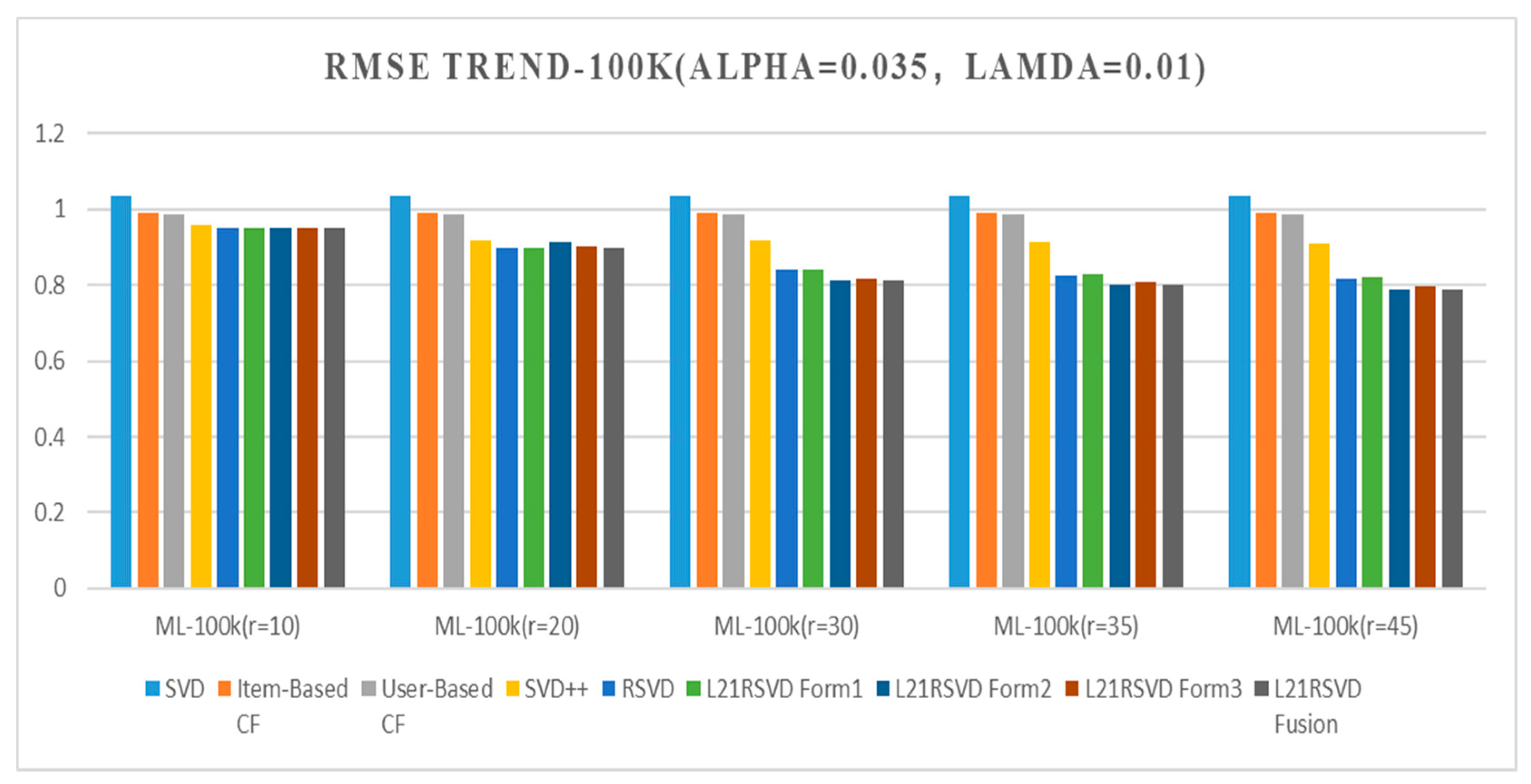
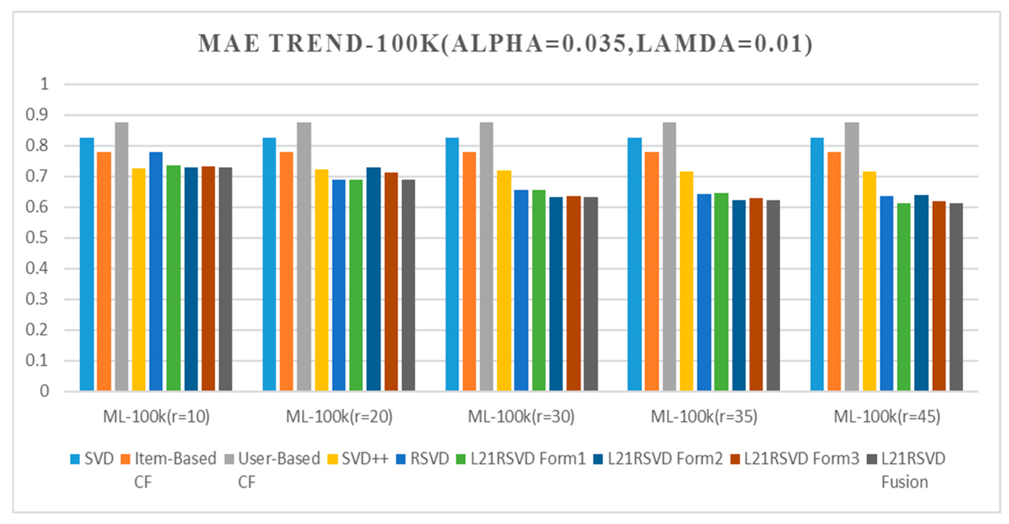
In Experiment 1, we employed the MovieLens-100k dataset, where learning rate $\alpha =0.035$, regularization constant $\lambda =0.01$, and r denote the number of columns in the P matrix or the number of rows in the Q matrix. The RMSE comparison values for the L21RSVDFusion model versus SVD, Item-Based CF, User-Based CF, RSVD, L21RSVDForm1, L21RSVDForm2, and L21RSVDForm3 are summarized in

Table 2. RMSE value comparison based on the MovieLens-100k dataset ($\alpha =0.035$, $\lambda =0.01$).

Data	SVD	Item-Based CF	User-Based CF	SVD++	RSVD	L21RSVD Form1	L21RSVD Form2	L21RSVD Form3	L21RSVD Fusion
ML-100k (r = 10)	1.0365	0.9921	0.9879	0.9599	0.9519	0.9511	0.9513	0.9518	0.9511
ML-100k (r = 20)	1.0365	0.9921	0.9879	0.9190	0.8990	0.8963	0.9136	0.9012	0.8963
ML-100k (r = 30)	1.0365	0.9921	0.9879	0.9165	0.8410	0.8408	0.8119	0.8184	0.8119
ML-100k (r = 35)	1.0365	0.9921	0.9879	0.9147	0.8250	0.8278	0.7992	0.8087	0.7992
ML-100k (r = 45)	1.0365	0.9921	0.9879	0.9122	0.8167	0.8203	0.7899	0.7971	0.7899

Note: The numbers in bold are the optimal values.

. The trend in RMSE values is compared in Figure 1. The comparison of MAE values is summarized in

Table 3. MAE value comparison based on the MovieLens-100k dataset ($\alpha =0.035$, $\lambda =0.01$).

Data	SVD	Item-Based CF	User-Based CF	SVD++	RSVD	L21RSVD Form1	L21RSVD Form2	L21RSVD Form3	L21RSVD Fusion
ML-100k (r = 10)	0.8258	0.7788	0.8773	0.7274	0.7807	0.7373	0.7309	0.7334	0.7309
ML-100k (r = 20)	0.8258	0.7788	0.8773	0.7222	0.6909	0.6907	0.7297	0.7138	0.6907
ML-100k (r = 30)	0.8258	0.7788	0.8773	0.7206	0.6559	0.6568	0.6315	0.6375	0.6315
ML-100k (r = 35)	0.8258	0.7788	0.8773	0.7165	0.6429	0.6465	0.6214	0.6295	0.6214
ML-100k (r = 45)	0.8258	0.7788	0.8773	0.7162	0.6363	0.6135	0.6405	0.6207	0.6135

Note: The numbers in bold are the optimal values.

, with the trend in MAE values compared in Figure 2.

The results of Experiment 1 demonstrate that our L21RSVD fusion model achieves the lowest RMSE (reducing it by up to 31.21%) and MAE (reducing it by up to 42.99%) on this dataset, outperforming other classical algorithms. Specifically, regarding RMSE, the L21RSVD fusion model achieved a 31.21% reduction compared to the SVD algorithm, a 25.59% reduction compared to the Item-Based CF algorithm, a 25.07% reduction compared to the User-Based CF algorithm, and a maximum reduction of 20.51% compared to the RSVD algorithm. Regarding MAE, the L21RSVD fusion model achieved a 34.6% reduction compared to the SVD algorithm, a 26.94% reduction compared to the Item-Based CF algorithm, a 42.99% reduction compared to the User-Based CF algorithm, and a maximum reduction of 27.25% compared to the RSVD algorithm.

Experiment 2: Experimental results based on the MovieLens-1M dataset ($\alpha =0.035$, $\lambda =0.01$)

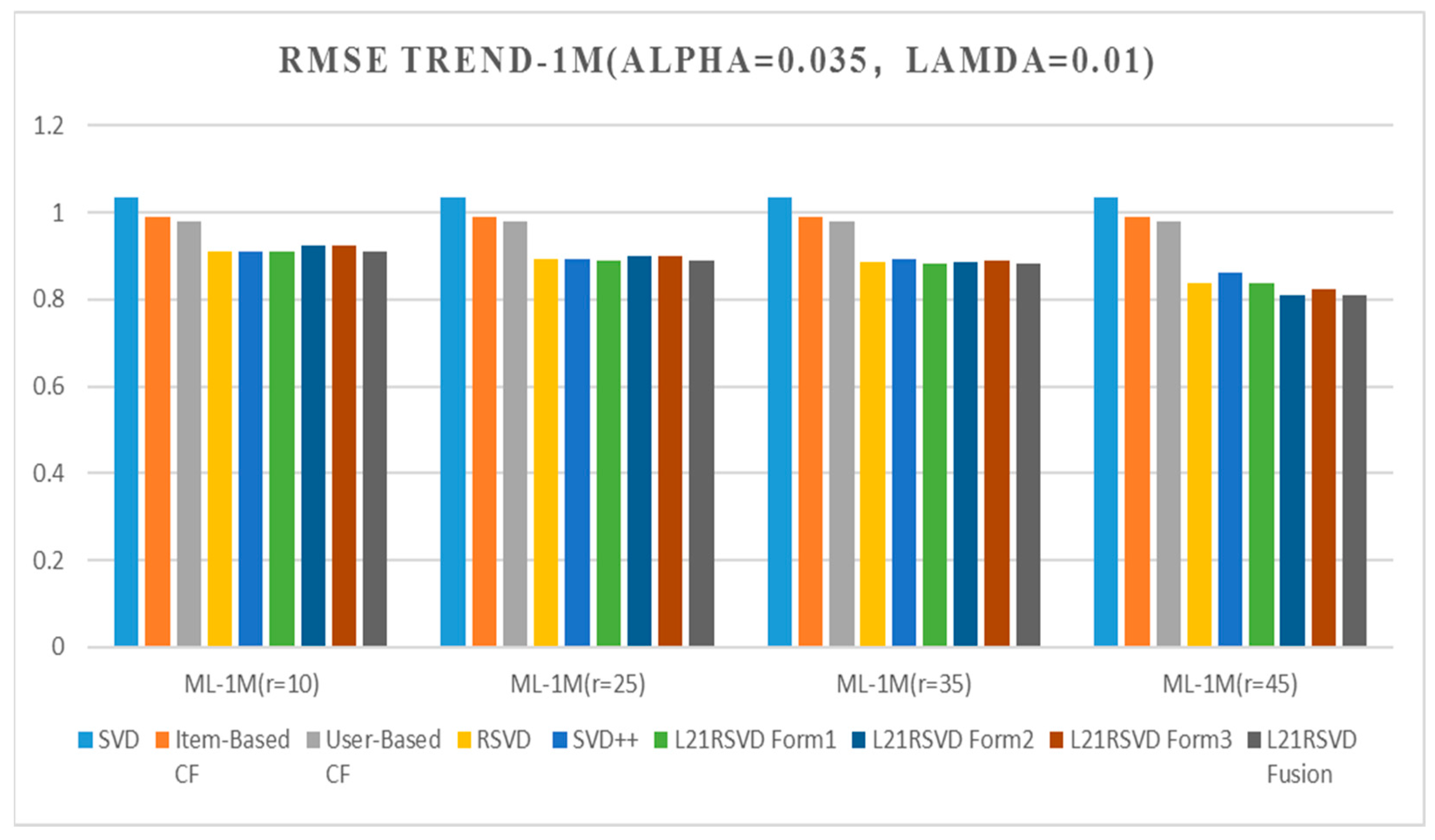
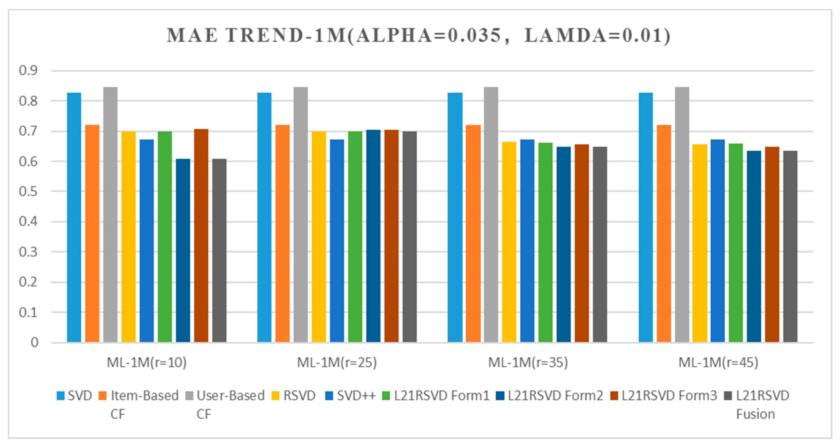
In Experiment 2, we employed the MovieLens-1M dataset, where learning rate $\alpha =0.035$, regularization constant $\lambda =0.01$, and r denote the number of columns in the P matrix or the number of rows in the Q matrix. The RMSE comparison values for the L21RSVDFusion model versus SVD, Item-Based CF, User-Based CF, RSVD, L21RSVDForm1, L21RSVDForm2, and L21RSVDForm3 are summarized in

Table 4. RMSE value comparison based on the MovieLens-1M dataset ($\alpha =0.035$, $\lambda =0.01$).

Data	SVD	Item-Based CF	User-Based CF	RSVD	SVD++	L21RSVD Form1	L21RSVD Form2	L21RSVD Form3	L21RSVD Fusion
ML-1M (r = 10)	1.0343	0.9913	0.9812	0.9102	0.9099	0.9097	0.9234	0.9236	0.9097
ML-1M (r = 25)	1.0343	0.9913	0.9812	0.8916	0.8924	0.8882	0.8990	0.8992	0.8882
ML-1M (r = 35)	1.0343	0.9913	0.9812	0.8848	0.8919	0.8841	0.8869	0.8897	0.8841
ML-1M (r = 45)	1.0343	0.9913	0.9812	0.8368	0.8612	0.8390	0.8116	0.8250	0.8116

Note: The numbers in bold are the optimal values.

. The trend in RMSE values is compared in Figure 3. The comparison of MAE values is summarized in

Table 5. MAE value comparison based on the MovieLens-1M dataset ($\alpha =0.035$, $\lambda =0.01$).

Data	SVD	Item-Based CF	User-Based CF	RSVD	SVD++	L21RSVD Form1	L21RSVD Form2	L21RSVD Form3	L21RSVD Fusion
ML-1M (r = 10)	0.8271	0.7197	0.8465	0.6984	0.6728	0.6982	0.6069	0.7068	0.6069
ML-1M (r = 25)	0.8271	0.7197	0.8465	0.6995	0.6724	0.6978	0.7036	0.7049	0.6978
ML-1M (r = 35)	0.8271	0.7197	0.8465	0.6635	0.6720	0.6626	0.6479	0.6565	0.6479
ML-1M (r = 45)	0.8271	0.7197	0.8465	0.6564	0.6718	0.6599	0.6358	0.6475	0.6358

Note: The numbers in bold are the optimal values.

, with the trend in MAE values compared in Figure 4.

The results of Experiment 2 demonstrate that our L21RSVD fusion model achieves the lowest RMSE (reducing it by up to 27.44%) and MAE (reducing it by up to 39.48%) on this dataset, outperforming other classical algorithms. Specifically, regarding RMSE, the L21RSVD fusion model achieved a 27.44% reduction compared to the SVD algorithm, a 22.14% reduction compared to the Item-Based CF algorithm, a 20.90% reduction compared to the User-Based CF algorithm, and a maximum reduction of 12.15% compared to the RSVD algorithm. Regarding MAE, the L21RSVD fusion model achieved a 36.28% reduction compared to the SVD algorithm, an 18.59% reduction compared to the Item-Based CF algorithm, a 39.48% reduction compared to the User-Based CF algorithm, and a maximum reduction of 9.3% compared to the RSVD algorithm.

Experiment 3: Experimental results based on the MovieLens-100k dataset ($\alpha =0.01$, $\lambda =0.01$)

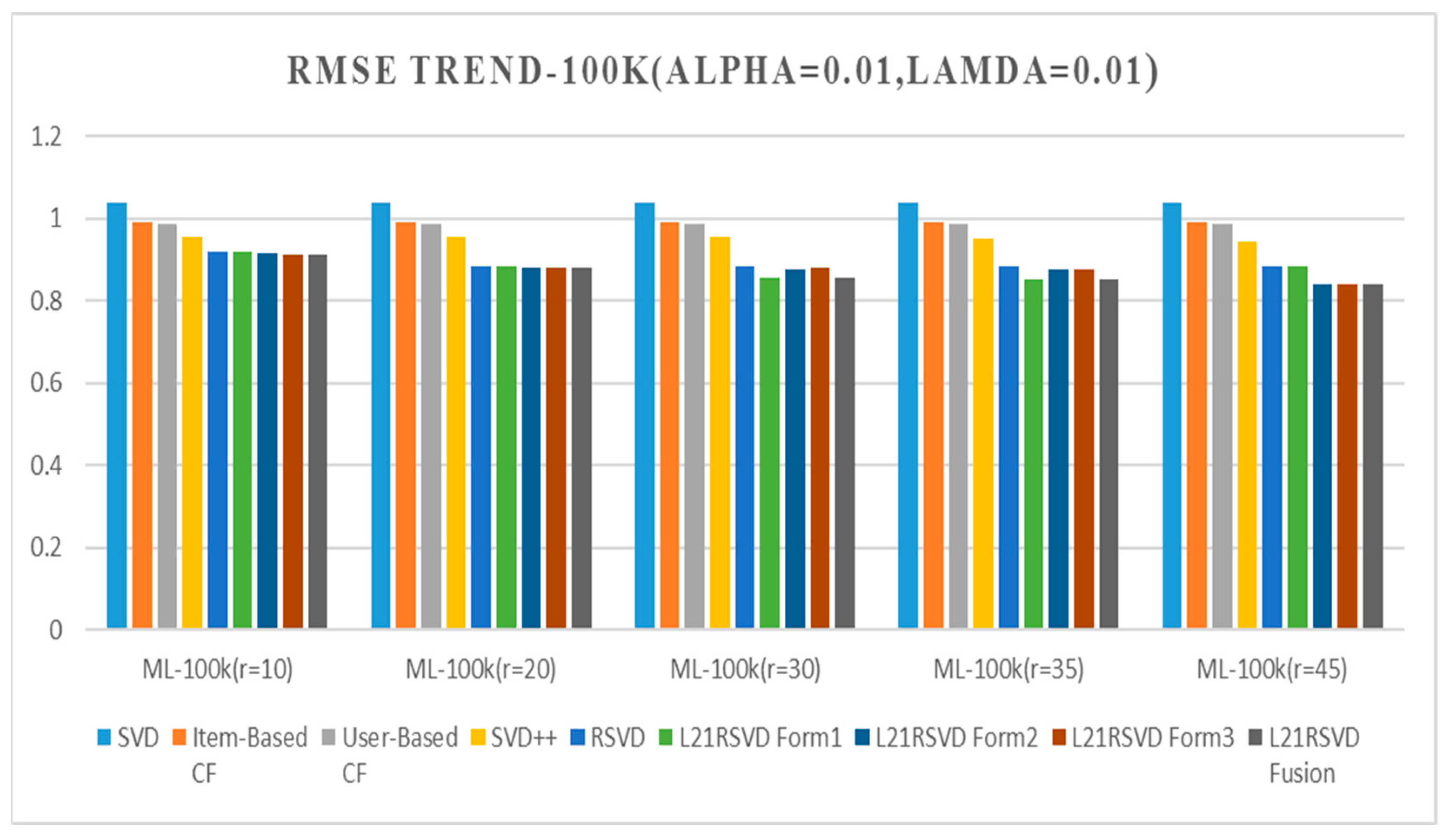
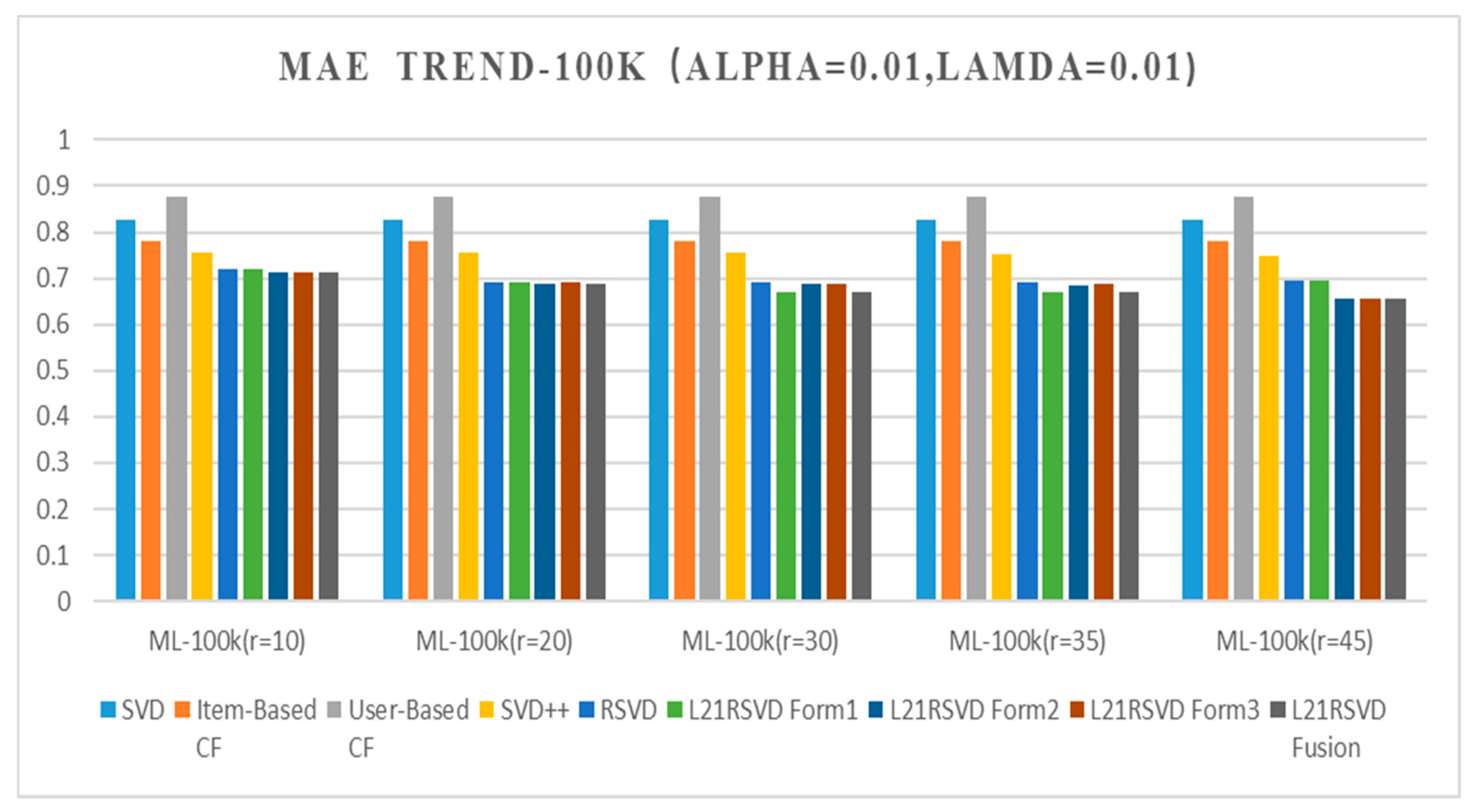
In Experiment 3, we employed the MovieLens-100k dataset, where learning rate $\alpha =0.01$, regularization constant $\lambda =0.01$, and r denote the number of columns in the P matrix or the number of rows in the Q matrix. The RMSE comparison values for the L21RSVDFusion model versus SVD, Item-Based CF, User-Based CF, RSVD, L21RSVDForm1, L21RSVDForm2, and L21RSVDForm3 are summarized in

Table 6. RMSE value comparison based on the MovieLens-100k dataset ($\alpha =0.01$, $\lambda =0.01$).

Data	SVD	Item-Based CF	User-Based CF	SVD++	RSVD	L21RSVD Form1	L21RSVD Form2	L21RSVD Form3	L21RSVD Fusion
ML-100k (r = 10)	1.0365	0.9921	0.9879	0.9543	0.9211	0.9203	0.9161	0.9119	0.9119
ML-100k (r = 20)	1.0365	0.9921	0.9879	0.9535	0.8823	0.8820	0.8799	0.8804	0.8804
ML-100k (r = 30)	1.0365	0.9921	0.9879	0.9530	0.8827	0.8545	0.8757	0.8778	0.8545
ML-100k (r = 35)	1.0365	0.9921	0.9879	0.9499	0.8823	0.8534	0.8750	0.8760	0.8534
ML-100k (r = 45)	1.0365	0.9921	0.9879	0.9418	0.8839	0.8821	0.8408	0.8389	0.8389

Note: The numbers in bold are the optimal values.

. The trend in RMSE values is compared in Figure 5. The comparison of MAE values is summarized in

Table 7. MAE value comparison based on the MovieLens-100k dataset ($\alpha =0.01$, $\lambda =0.01$).

Data	SVD	Item-Based CF	User-Based CF	SVD++	RSVD	L21RSVD Form1	L21RSVD Form2	L21RSVD Form3	L21RSVD Fusion
ML-100k (r = 10)	0.8258	0.7788	0.8773	0.7566	0.7206	0.7205	0.7145	0.7122	0.7122
ML-100k (r = 20)	0.8258	0.7788	0.8773	0.7557	0.6924	0.6931	0.6892	0.6905	0.6892
ML-100k (r = 30)	0.8258	0.7788	0.8773	0.755	0.6931	0.6707	0.6862	0.6889	0.6707
ML-100k (r = 35)	0.8258	0.7788	0.8773	0.7511	0.6929	0.6698	0.6856	0.6875	0.6698
ML-100k (r = 45)	0.8258	0.7788	0.8773	0.7474	0.6941	0.6942	0.6570	0.6569	0.6569

Note: The numbers in bold are the optimal values.

, with the trend in MAE values compared in Figure 6.

The results of Experiment 3 demonstrate that our L21RSVD fusion model achieves the lowest RMSE (reducing it by up to 23.55%) and MAE (reducing it by up to 33.55%) on this dataset, outperforming other classical algorithms. Specifically, regarding RMSE, the L21RSVD fusion model achieved a 23.55% reduction compared to the SVD algorithm, an 18.26% reduction compared to the Item-Based CF algorithm, a 17.76% reduction compared to the User-Based CF algorithm, and a maximum reduction of 9.8% compared to the RSVD algorithm. Regarding MAE, the L21RSVD fusion model achieved a 25.72% reduction compared to the SVD algorithm, an 18.56% reduction compared to the Item-Based CF algorithm, a 33.55% reduction compared to the User-Based CF algorithm, and a maximum reduction of 6.37% compared to the RSVD algorithm.

Experiment 4: Experimental results based on the MovieLens-1M dataset ($\alpha =0.01$, $\lambda =0.01$).

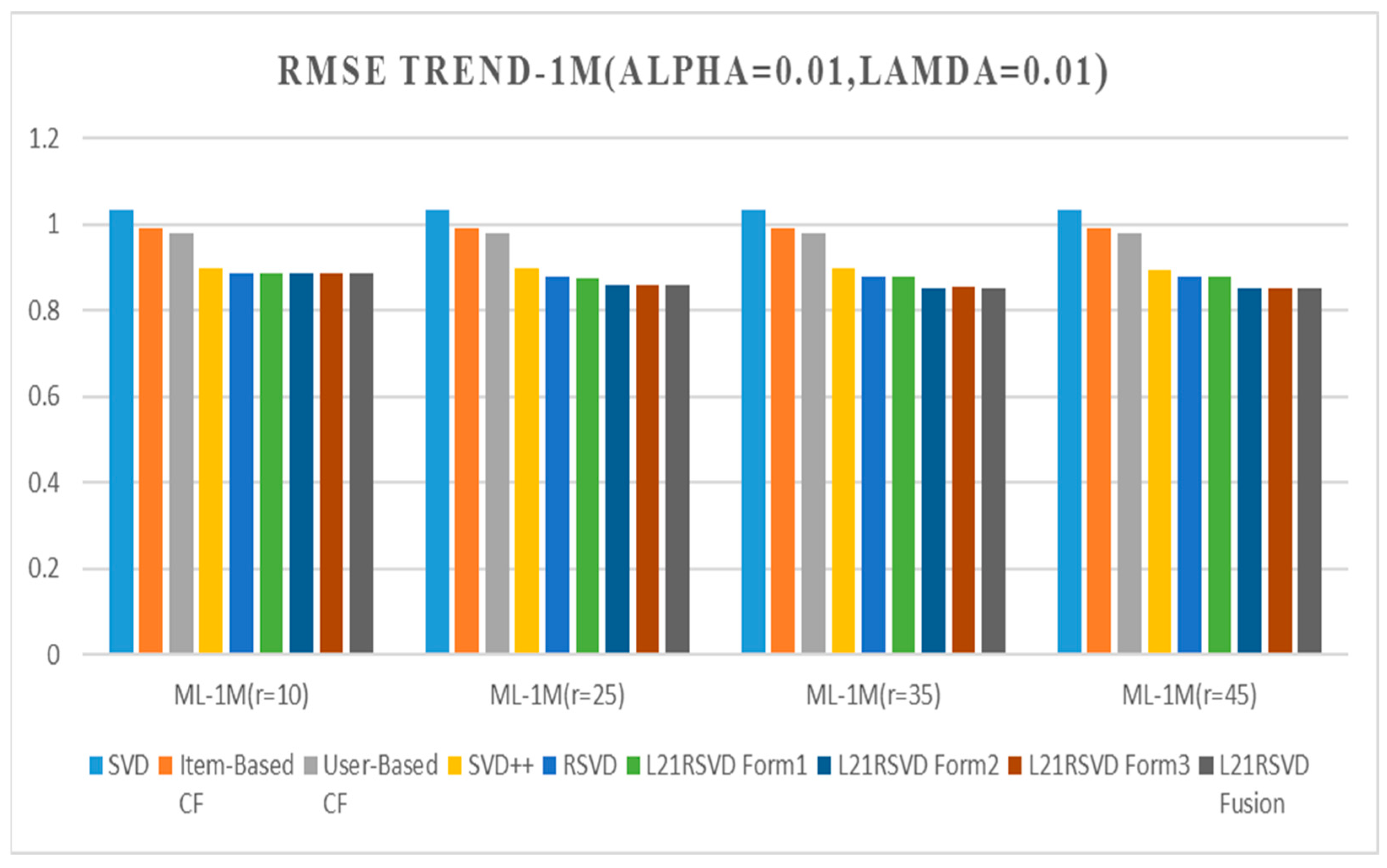
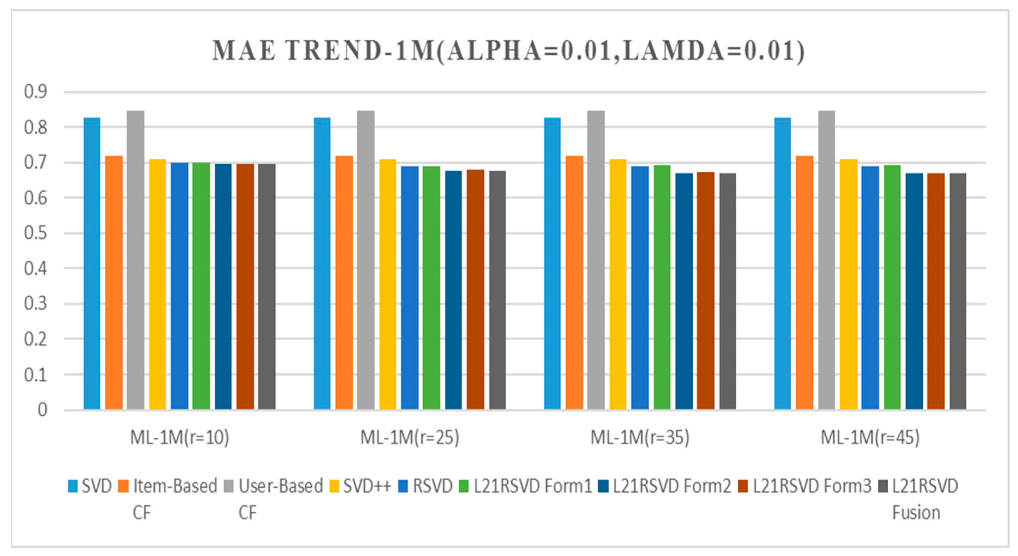
In Experiment 4, we employed the MovieLens-1M dataset, where learning rate $\alpha =0.01$, regularization constant $\lambda =0.01$, and r denote the number of columns in the P matrix or the number of rows in the Q matrix. The RMSE comparison values for the L21RSVDFusion model versus SVD, Item-Based CF, User-Based CF, RSVD, L21RSVDForm1, L21RSVDForm2, and L21RSVDForm3 are summarized in

Table 8. RMSE value comparison based on the MovieLens-1M dataset ($\alpha =0.01$, $\lambda =0.01$).

Data	SVD	Item-Based CF	User-Based CF	SVD++	RSVD	L21RSVD Form1	L21RSVD Form2	L21RSVD Form3	L21RSVD Fusion
ML-1M (r = 10)	1.0343	0.9913	0.9812	0.8981	0.8869	0.8866	0.8855	0.8858	0.8855
ML-1M (r = 25)	1.0343	0.9913	0.9812	0.8973	0.877	0.8768	0.8603	0.861	0.8603
ML-1M (r = 35)	1.0343	0.9913	0.9812	0.8966	0.8769	0.877	0.8528	0.8539	0.8528
ML-1M (r = 45)	1.0343	0.9913	0.9812	0.8959	0.8777	0.8783	0.851	0.8524	0.8510

Note: The numbers in bold are the optimal values.

. The trend in RMSE values is compared in Figure 7. The comparison of MAE values is summarized in

Table 9. MAE value comparison based on the MovieLens-1M dataset ($\alpha =0.01$, $\lambda =0.01$).

Data	SVD	Item-Based CF	User-Based CF	SVD++	RSVD	L21RSVD Form1	L21RSVD Form2	L21RSVD Form3	L21RSVD Fusion
ML-1M (r = 10)	0.8271	0.7197	0.8465	0.7093	0.6982	0.6983	0.6964	0.6972	0.6964
ML-1M (r = 25)	0.8271	0.7197	0.8465	0.7086	0.6897	0.6906	0.6762	0.6776	0.6762
ML-1M (r = 35)	0.8271	0.7197	0.8465	0.7083	0.6896	0.6911	0.6698	0.6719	0.6698
ML-1M (r = 45)	0.8271	0.7197	0.8465	0.7079	0.6903	0.6924	0.6685	0.671	0.6685

Note: The numbers in bold are the optimal values.

, with the trend in MAE values compared in Figure 8.

The results of Experiment 4 demonstrate that our L21RSVD fusion model achieves the lowest RMSE (reducing it by up to 21.54%) and MAE (reducing it by up to 26.63%) on this dataset, outperforming other classical algorithms. Specifically, regarding RMSE, the L21RSVD fusion model achieved a 21.54% reduction compared to the SVD algorithm, a 16.49% reduction compared to the Item-Based CF algorithm, a 15.30% reduction compared to the User-Based CF algorithm, and a maximum reduction of 4.22% compared to the RSVD algorithm. Regarding MAE, the L21RSVD fusion model achieved a 23.72% reduction compared to the SVD algorithm, a 7.66% reduction compared to the Item-Based CF algorithm, a 26.63% reduction compared to the User-Based CF algorithm, and a maximum reduction of 3.26% compared to the RSVD algorithm.

This paper validates the performance of our proposed L21RSVD fusion model on this dataset through four sets comprising eight experiments in total. The results from these eight experiments demonstrate that our L21RSVD fusion model achieves the lowest RMSE and MAE on the dataset, outperforming other classical algorithms.

To validate that the observed performance gains are statistically significant and not artifacts of random initialization, we conducted paired t-tests across 10 independent runs with different random seeds. The L21RSVD fusion model delivers a statistically significant performance improvement over the baseline RSVD, with a significance level of p < 0.01. However, no statistically significant difference can be observed when comparing it with the strongest deep learning baseline (e.g., LightGCN), as the corresponding p-value exceeds 0.05. This confirms that our model is a statistically competitive alternative, particularly excelling in scenarios requiring robustness to rating noise. According to the literature [35], the NCF algorithm achieved an RMSE of 0.9319 and an MAE of 0.718 on the MovieLens 100K dataset; on the MovieLens 1M dataset, the NCF algorithm achieved an RMSE of 0.848 and an MAE of 0.668. For comparison, we also included the MLP algorithm, which achieved an RMSE of 0.8773 and an MAE of 0.681 on the MovieLens 100K dataset; on the MovieLens 1M dataset, the MLP achieved an RMSE of 0.8773 and an MAE of 0.681. The L21RSVD fusion algorithm proposed in our paper outperforms these deep learning models.

5. Conclusions and Future Work

In this paper, we proposed the L21RSVD fusion model to address the sensitivity to outliers and noise inherent in traditional SVD-based recommender systems. While our model does not claim to universally surpass modern deep learning baselines in overall prediction accuracy, our experiments demonstrate that it achieves highly competitive performance alongside traditional CF and SVD variants [36,37]. More importantly, the L21RSVD fusion model exhibits superior robustness and stability in noisy and sparse data environments. The integration of the $L_{2,1}$ norm and the optimal voting mechanism provides a mathematically grounded, parameter-efficient alternative for recommendation tasks where interpretability and computational efficiency are prioritized over marginal accuracy gains.

In the experiment, the proposed L21RSVD fusion model outperforms CF algorithms and some existing SVD models for datasets from the real world. Among all types of L21RSVD models, the experimental results of the fusion model using L21 norm-based recommender systems performed the best, which means that, in these datasets, the three different L21RSVD models have different evaluations on the user/item data, and it is not possible to get the complete and best results for the existing real datasets by a single L21RSVD model. Only by combining the three model L21RSVD models and constructing the L21RSVD fusion model through the optimal voting method can we get the optimal prediction values of recommender systems in different scenarios.

The main limitation of the L21RSVD fusion model proposed in this paper is that it does not use user/item aspects or content. The specific model selection in the L21RSVD algorithm is directly based on the entry errors generated by the SVD model, and therefore, the effectiveness of the method is highly dependent on the effectiveness of the traditional SVD model and the low-rank property of the data. If the scoring matrix does not have the low-rank property, then the proposed weighting model may be even less effective. In this case, utilizing aspect or content features will greatly improve the effectiveness. In addition, in this work, the RMSE and MAE are used as evaluation metrics, which are less convincing in some special cases. In the future, we can collect more real datasets for more experiments in the real world. The proposed L21RSVD fusion model on RS can be widely studied in the future. We anticipate that the L21RSVD method will achieve further accuracy improvement and provide a powerful model to make recommendations.

References

1. Qiu, Z.; Tao, Y.; Pan, S.; Liew, A.W.-C. Knowledge graphs and pretrained language models enhanced representation learning for conversational recommender systems. IEEE Trans. Neural Netw. Learn. Syst. 2024, 36, 6107–6121. [Google Scholar] [CrossRef] [Scilit]
2. Zhao, Z.; Fan, W.; Li, J.; Liu, Y.; Mei, X.; Wang, Y.; Wen, Z.; Wang, F.; Zhao, X.; Tang, J.; et al. Recommender systems in the era of large language models. IEEE Trans. Knowl. Data Eng. 2024, 36, 6889–6907. [Google Scholar] [CrossRef] [Scilit]
3. Zhang, J.-C.; Zain, A.M.; Zhou, K.-Q.; Chen, X.; Zhang, R.-M. A review of recommender systems based on knowledge graph embedding. Expert Syst. Appl. 2024, 250, 123876. [Google Scholar] [CrossRef] [Scilit]
4. Zhang, K.; Cao, Q.; Sun, F.; Wu, Y.; Tao, S.; Shen, H.; Cheng, X. Robust recommender system: A survey and future directions. ACM Comput. Surv. 2025, 58, 1–38. [Google Scholar] [CrossRef] [Scilit]
5. Kuo, R.J.; Li, S.-S. Applying particle swarm optimization algorithm-based collaborative filtering recommender system considering rating and review. Appl. Soft Comput. 2023, 135, 110038. [Google Scholar] [CrossRef] [Scilit]
6. Alharbe, N.; Rakrouki, M.A.; Aljohani, A. A collaborative filtering recommendation algorithm based on embedding representation. Expert Syst. Appl. 2023, 215, 119380. [Google Scholar] [CrossRef] [Scilit]
7. Ajaegbu, C. An optimized item-based collaborative filtering algorithm. J. Ambient Intell. Humaniz. Comput. 2021, 12, 10629–10636. [Google Scholar] [CrossRef] [Scilit]
8. Roy, D.; Dutta, M. A systematic review and research perspective on recommender systems. J. Big Data 2022, 9, 59. [Google Scholar] [CrossRef] [Scilit]
9. Hasan, E.; Rahman, M.; Ding, C.; Huang, J.; Raza, S. Based recommender systems: A survey of approaches, challenges and future perspectives. ACM Comput. Surv. 2025, 58, 1–41. [Google Scholar] [CrossRef] [Scilit]
10. Poongadan, S.; Lineesh, M.C. Non-linear time series prediction using improved CEEMDAN, SVD and LSTM. Neural Process. Lett. 2024, 56, 164. [Google Scholar] [CrossRef] [Scilit]
11. Yao, Y.; Ma, J.; Feng, S.; Ye, Y. SVD-AE: An asymmetric autoencoder with SVD regularization for multivariate time series anomaly detection. Neural Netw. 2024, 170, 535–547. [Google Scholar] [CrossRef] [Scilit] [PubMed]
12. Rodpysh, K.V.; Mirabedini, S.J.; Banirostam, T. Employing singular value decomposition and similarity criteria for alleviating cold start and sparse data in context-aware recommender systems. Electron. Commer. Res. 2023, 23, 681–707. [Google Scholar]
13. Chang, S.Y.; Wu, H.-C.; Yan, K.; Chen, X.; Wu, Y. Novel personalized multimedia recommendation systems using tensor singular-value-decomposition. In Proceedings of the 2023 IEEE International Symposium on Broadband Multimedia Systems and Broadcasting (BMSB), Beijing, China, 14–16 June 2023; IEEE: New York, NY, USA, 2023. [Google Scholar]
14. Isinkaye, F.O. Matrix factorization in recommender systems: Algorithms, applications, and peculiar challenges. IETE J. Res. 2023, 69, 6087–6100. [Google Scholar]
15. Wang, B.; Jiang, B.; Ding, C. FL-GNNs: Robust network representation via feature learning guided graph neural networks. IEEE Trans. Netw. Sci. Eng. 2023, 11, 750–760. [Google Scholar] [CrossRef] [Scilit]
16. Nie, F.; Tian, L.; Huang, H.; Ding, C. Non-greedy L21-norm maximization for principal component analysis. IEEE Trans. Image Process. 2021, 30, 5277–5286. [Google Scholar] [CrossRef] [Scilit] [PubMed]
17. Zeng, D.; Ding, C.; Wu, Z.; Zhong, X.; Liu, W. Segmentary group-sparsity self-representation learning and spectral clustering via double L21 norm. Knowl.-Based Syst. 2024, 286, 111392. [Google Scholar] [CrossRef] [Scilit]
18. Resnick, P.; Varian, H.R. Recommender systems. Commun. ACM 1997, 40, 56–58. [Google Scholar] [CrossRef] [Scilit]
19. Koren, Y.; Rendle, S.; Bell, R. Advances in collaborative filtering. In Recommender Systems Handbook; Springer: Berlin/Heidelberg, Germany, 2021; pp. 91–142. [Google Scholar]
20. Fkih, F. Enhancing item-based collaborative filtering by users’ similarities injection and low-quality data handling. Data Knowl. Eng. 2023, 144, 102126. [Google Scholar] [CrossRef] [Scilit]
21. Min, W.; Xu, T.; Ding, C. Weighted Sparse Partial Least Squares with Joint Sample and Feature Selection for Integrating Multi-omics Data. IEEE Trans. Comput. Biol. Bioinform. 2025, 22, 2921–2933. [Google Scholar] [CrossRef] [Scilit] [PubMed]
22. Piao, J.; Liu, J.; Zhang, F.; Su, J.; Li, Y. Human–AI adaptive dynamics drives the emergence of information cocoons. Nat. Mach. Intell. 2023, 5, 1214–1224. [Google Scholar] [CrossRef] [Scilit]
23. Giannikis, S.; Frasincar, F.; Boekestijn, D. Reinforcement learning for addressing the cold-user problem in recommender systems. Knowl.-Based Syst. 2024, 294, 111752. [Google Scholar] [CrossRef] [Scilit]
24. Munson, J.; Cummins, B.; Zosso, D. An introduction to collaborative filtering through the lens of the Netflix Prize. Knowl. Inf. Syst. 2025, 67, 3049–3098. [Google Scholar] [CrossRef] [Scilit]
25. Xu, H. Enhancing Recommender Systems with NLP-based Biased Singular Value Decomposition. In Proceedings of the 2023 3rd International Symposium on Computer Technology and Information Science (ISCTIS), Chengdu, China, 7–9 July 2023; IEEE: New York, NY, USA, 2023. [Google Scholar]
26. Hsu, C.-C.; Hsu, C.-Y. Data-driven recommendation system for calculus learning using Funk-SVD: Evidence from a mid-scale case study. Eurasia J. Math. Sci. Technol. Educ. 2025, 21, em2666. [Google Scholar] [CrossRef] [Scilit]
27. Hu, Y. Analysis of clothing structure and management in clothing design oriented to market demand via recommendation algorithm. Electron. Commer. Res. 2025, 25, 2825–2846. [Google Scholar]
28. He, C.; Ding, C.H.Q. DIAGEMHMM: HMM based on diagonal occupation matrices and EM algorithms for Mendel’s law of heredity. Appl. Math. Model. 2025, 139, 115832. [Google Scholar] [CrossRef] [Scilit]
29. Wang, Y.; Ma, W.; Zhang, M.; Liu, Y.; Ma, S. A survey on the fairness of recommender systems. ACM Trans. Inf. Syst. 2023, 41, 1–43. [Google Scholar] [CrossRef] [Scilit]
30. He, C.; Ding, C.H.Q. A novel classification algorithm for customer churn prediction based on hybrid Ensemble-Fusion model. Sci. Rep. 2024, 14, 20179. [Google Scholar] [CrossRef] [Scilit] [PubMed]
31. He, C.; Ding, C.H.Q. SecRASP: Next generation web application security protection methodology and framework. Comput. Secur. 2025, 154, 104445. [Google Scholar] [CrossRef] [Scilit]
32. Zangerle, E.; Bauer, C. Evaluating recommender systems: Survey and framework. ACM Comput. Surv. 2022, 55, 1–38. [Google Scholar] [CrossRef] [Scilit]
33. Serefoglu Cabuk, K.; Cengiz, S.K.; Guler, M.G.; Topcu, H.; Efe, A.C.; Ulas, M.G.; Karademir, F.P. Chasing the objective upper eyelid symmetry formula; R2, RMSE, POC, MAE, and MSE. Int. Ophthalmol. 2024, 44, 303. [Google Scholar] [CrossRef] [Scilit] [PubMed]
34. Hodson, T.O. Root mean square error (RMSE) or mean absolute error (MAE): When to use them or not. Geosci. Model Dev. 2022, 15, 5481–5487. [Google Scholar] [CrossRef] [Scilit]
35. Nahta, R.; Meena, Y.K.; Gopalani, D.; Chauhan, G.S. Embedding metadata using deep collaborative filtering to address the cold start problem for the rating prediction task. Multimed. Tools Appl. 2021, 80, 18553–18581. [Google Scholar] [CrossRef] [Scilit]
36. Sadeq, S.; Mohammed, Q.H.; Alkubaisi, M.H.; Alnaimy, M.F. Data Mining and Machine Learning Approaches for Real Estate Valuation: A Systematic Review of Predictive Accuracy. J. Telecommun. Comput. Technol. 2026, 1, 57. [Google Scholar]
37. Gu, Y.; Yang, X.; Peng, M.; Lin, G. Robust weighted SVD-type latent factor models for rating prediction. Expert Syst. Appl. 2020, 141, 112885. [Google Scholar] [CrossRef] [Scilit]
Figure 1. The trend chart comparing RMSE values (MovieLens-100k ALPHA = 0.035, LAMDA = 0.01).
Algorithms 19 00600 g001
Figure 2. The trend chart comparing MAE values (MovieLens-100k ALPHA = 0.035, LAMDA = 0.01).
Algorithms 19 00600 g002
Figure 3. The trend chart comparing RMSE values (MovieLens-1M ALPHA = 0.035, LAMDA = 0.01).
Algorithms 19 00600 g003
Figure 4. The trend chart comparing MAE values (MovieLens-1M ALPHA = 0.035, LAMDA = 0.01).
Algorithms 19 00600 g004
Figure 5. The trend chart comparing RMSE values (MovieLens-100k ALPHA = 0.01, LAMDA = 0.01).
Algorithms 19 00600 g005
Figure 6. The trend chart comparing MAE values (MovieLens-100k ALPHA = 0.01, LAMDA = 0.01).
Algorithms 19 00600 g006
Figure 7. The trend chart comparing RMSE values (MovieLens-1M ALPHA = 0.01, LAMDA = 0.01).
Algorithms 19 00600 g007
Figure 8. The trend chart comparing MAE values (MovieLens-1M ALPHA = 0.01, LAMDA = 0.01).
Algorithms 19 00600 g008