Explorations on Improving Interpretability of Decision Making Processes of Rule-Based Classifiers

Abstract

Rule-based classifiers are often preferred over other types of learners due to the transparent mode in which decisions are made. Each decision rule includes in its premise conditions on attributes. When they are satisfied, the conclusion part of the rule comes into play and leads to assigning an object to a specific class. Following the classification process is relatively straightforward but can become more complex when the cardinality of rule set is high. Furthermore, when rules are induced from continuous data, the conditions listed belong to this domain as well, which makes them less general. This paper presents an illustrative example for the exploratory research methodology where the sets of rules are induced in the continuous input domain, but next, they are transformed by discretisation procedures, which results in a simplified representation of the data and knowledge patterns learnt. In addition, the rule sets are also filtered based on rankings obtained for variants of the transformed data. The processing results in reduced decision algorithms with categorical conditions. This simplification is advantageous in and of itself, but the experiments carried out on datasets in the stylometric domain show that it can also lead to enhanced performance of rule-based classifiers.

1. Introduction

Reducing the complexity of a data model is an important step on the way to achieving interpretability of a decision making process [1]. Dimensionality reduction is a widely studied problem, with permanently increasing importance due to constantly accumulating amounts of data, which also increase in volume. With too many descriptive features to choose from, their relevance for any given task and the characteristics of a domain can become lost under information overload and work to disadvantage rather than help in understanding the properties of the data and leading to effective knowledge discovery.

Simplification of a space under consideration is a challenge that can be approached in many ways and directed at various aspects. Feature selection algorithms can be employed to provide some insight into importance of variables, evaluated outside or in addition to expert knowledge [2]. The ranking mechanisms, which can be embedded in the data exploration or applied in the data preprocessing stage, organise the available attributes into ordered lists, from the most relevant to the least relevant elements. This list can be exploited to retrieve only a subset of features found to be the most interesting or most important for the problem under study [3].

Characteristics of the input space, and dependencies and patterns that can be detected change when this space is transformed. Discretisation is a process that aims essentially at the simplification of data while preserving some part of the informative content [4]. The continuous space is partitioned into ranges of values, and datapoints are represented by the corresponding intervals defined along the way. Typically, discretisation is considered among data preprocessing methods and applied in the initial preparation stage. The categorical attributes obtained make data mining less demanding, and a wider range of approaches can handle them due to much simplified calculations. However, knowledge discovery based on discretised data means learning in conditions where some information becomes inaccessible. Supervised discretisation algorithms, by their focus on class distinction, are capable of rejecting attributes by assigning a single interval to represent their entire domains [5], which means operation as a feature reduction method.

Taking advantage of both reasoning from all available data and simplification resulting from discretisation means reversing the order of standard processing steps [6]. Instead of first preparing the data and then exploring them, discretisation can follow knowledge discovery. Yet, for this approach to work, the patterns extracted from the data need to be directly accessible; therefore, the methodology can be applied only in the situation of transparent representation of learnt knowledge. Such is the case with sets of decision rules.

In the field of supervised machine learning, rule-based classifiers are often preferred over other approaches, even at the cost of lowered expectations with respect to performance. This is due to the relatively easy interpretability of the decision making process. Each decision rule directly shows the premises on which a decision is made. Induction algorithms search for rules and return their sets of varied cardinalities, which can, next, be applied to labelling unknown samples. With many rules firing for a sample, a conflict can occur that needs to be resolved by some strategy [7], such as voting. When the numbers of inferred rules are high, the operation of a rule-based classifier is more complex and takes more time. To counteract this, pruning of rule sets can be attempted [8]. Individual rules are evaluated with some measure that reflects their quality, and then only the subset is selected. In the research presented in this paper, three mechanisms were examined with the aim of improving the interpretability of a decision making process for rule-based classifiers. These simplification approaches included discretisation of the data, transformations of the knowledge patterns learnt, and rule filtering combined with feature selection based on attribute rankings.

Operating in stylometry as an application domain [9], two datasets with numerical attributes were prepared for an exploratory analysis of writing styles. Each dataset represented a task of binary authorship attribution based on linguistic preferences and habits of authors, represented through stylometric features [10]. From the continuous input space, the sets of decision rules were induced by the Dominance-Based Rough Set Approach (DRSA) [11]. DRSA is an extension of the classical rough set approaches invented by Pawlak [12] that could handle only nominal or discrete data. By incorporating dominance relation, the Dominance-Based Rough Set Approach can process directly numerical attributes and returns sets of decision rules including conditions on them in their premises.

Within the illustrated methodology, the conditions in the inferred rules were discretised by replacing them with the corresponding categorical representations found in transformations of the data, which caused a noticeable simplification and enhanced generalisation properties of the rules. Several discretisation approaches were applied to the data and patterns: the Kononenko algorithm [13] of the supervised category and several variants of equal-frequency and equal-width binning from the group of unsupervised methods. For all investigated domains, continuous and discrete, the sets of decision rules were filtered. The selection process was controlled by rankings of attributes to include information on their relevance in considerations. In all filtering procedures, the performance of rule classifiers was evaluated with test sets discretised by two modes of transformation, independent and dependent, and examined in the context of two strategies of conflict resolution, weighted voting versus simple majority voting.

The described research expanded on the results obtained in previous experiments [14]. In the earlier works, as discretisation approaches, the algorithm by Fayyad and Irani and variants of equal frequency binning were employed. Classifier performance was evaluated only with dependently transformed test sets. Weighted voting was used as the only available conflict resolution strategy. This paper includes new directions and elements of the methodology by exploiting different discretisation methods, considering transformations adapted to sets used for evaluation of classifiers, examining the influence of conflicts occurring when many rules fire for a sample, and the characteristics of reduced rule sets.

The experimental results show the merits of the methodology presented. In most of the rule filtering procedures executed, some conditions for improved interpretability were detected while at the same time at least preserving, but also increasing, the power of rule-based classifiers. The improvement was visible in rule premises simplified by discretisation, and in noticeably smaller rule sets retrieved after filtering.

The main contributions of this paper are as follows.

• Presentation of the research methodology where the representation of knowledge discovered by data mining was transformed by discretisation;
• Investigation into an application of simplification approaches to the process of decision making by rule-based classifiers;
• Study of rule filtering executed in various directions and with different rule selection strategies;
• Examination of the influence of various operation conditions while labelling samples using rule-based classifiers.

The content of the paper was prepared as follows. Section 2 describes the research background and an explanation of the methodology used in the experiments. Section 3 includes comments on the results obtained, with the discussion provided in Section 4, while Section 5 concludes the paper.

2. Materials and Methods

The research reported in this paper involved the application of some simplification approaches to the task of decision making by rule-based classifiers. The simplification included transformations of the considered input space and also knowledge patterns discovered there by discretisation, and filtering sets of decision rules induced from the data. The section presents all elements of the background, as well as a description of the experimental setup, giving the scope and extent of investigations.

2.1. Decision Making Process of Rule-Based Classifiers

One of the key elements needed for effective data mining is understanding how the decision making process works and being able to interpret the knowledge patterns discovered by explorations [15]. Among a multitude of methods and algorithms that belong to supervised machine learning, rule-based classifiers deserve special mention because not only can they be used to label unknown samples but they also provide direct access to learnt knowledge represented by inferred rules, and the act of reaching a conclusion based on given premises is always completely transparent [16].

A decision rule of the $If\dots then$ form consists of two parts. The premise includes the conjunction of descriptors, pairs of attribute–value, which give conditions on attributes. The conclusion provides the decision with respect to the assigned class, when all listed conditions are met. The number of conditions is referred to as the length of the rule, which is an important characteristic. Shorter rules are less detailed, and therefore, they possess better generalisation properties [17]. Longer rules describe some training data closely, sometimes too closely, which can lead to overfitting. A decision rule is discriminative with respect to classes when, for all covered training samples, that is, those with attribute values matching conditions, the assigned labels also match. Such covered samples support decisions based on the listed premise; therefore, this term is used as another important rule characteristic. The higher the value of the rule support, the more often it occurs or it represents a major pattern, while lower supports indicate some minor patterns described by the rules.

To infer decision rules, an induction algorithm needs to process values that comprise domains of attributes. The nature of the input domain reflects the relational operators used in the descriptors. Some approaches work only for nominal or discrete data, and then, the operator is that of equality. When attributes are numerical, either discretisation must precede the search for rules, or the rule induction algorithm must be able to handle real values [18]. In the latter case, the range of operators can then be extended to include some elements of the set $\{=,\ne ,<,\le ,>,\ge ,\in \}$, leading to consideration of ordered attribute values or comparisons with a set or range of values.

When decision rules are inferred from the input data, they can be next applied in the process of assigning class labels to unknown samples. For all yet unattributed examples, rules that cover them are sought. If for a sample, a single rule is found with conditions that match the values of attributes included, then its decision attribute gives the corresponding class label. When several rules cover the sample, the question of labelling can become more complex, depending on agreement or lack of it, between individual decisions provided by firing rules. When all matching rules point to one and the same class, then they can kind of support each other in the process of reaching the final decision. If, however, some rules disagree on where a sample should be assigned, the resulting conflict must be resolved by some strategy [19].

The most radical strategy would be to treat all samples with ambiguous decisions caused by conflicts as unattributed, without the final decision about how they are classified. In consequence of such processing, only the samples with unanimous decisions reached by covering decision rules would be labelled. In cases where the sets of rules have a high cardinality, that could possibly mean even zero decisions. Furthermore, with this approach, the samples not covered could not be distinguished from those covered but by conflicting rules, which do not correctly reflect the characteristics of knowledge discovery [20]. When there is no coverage, it means that the patterns represented by the sample under study were absent in the data from which the rules were induced. A conflict shows that a sample is representative of multiple detected patterns, characteristic to not one but various classes.

Another tactic leads to exploiting mechanisms typically associated with collaborative decision making [21]. Decisions of all matching rules are considered as if they were submitted by elementary inducers, and some form of voting returns the needed final verdict. If each rule is assigned a single vote, regardless of its characteristics, and the class with the highest number of votes is chosen as the final label, then simple majority voting is applied. Disregarding the issue of rule quality can cause the situation where weaker rules outvote stronger rules simply because they are more numerous. An alternative procedure is provided by weighted voting. Each decision rule is assigned as many votes as its support, and then, the votes are calculated. With this approach, decisions submitted by stronger rules are reinforced to reflect the dominance of patterns represented by them.

Information on the extent of decisions that need to be reached through some strategy due to clashing assignments given by firing rules can be provided by the conflict rate. It can be expressed as a fraction of samples from a set under study for which conflicts occurred. A conflict rate equal zero means that when there are rules matching an example, they always agree on the decision. A conflict rate equal to one denotes the case where for all covered samples, at least one rule disagrees with the others with respect to the assigned class label. However, lower values of the conflict rate should not be interpreted as leading to higher accuracy, since the lack of conflict is not equivalent to only correct decisions being made. Therefore, this characteristic rather reflects the overall complexity of a decision making process for a classifier.

2.2. Exploration of Data with Dominance-Based Rough Set Approach

In a rough set perspective, the universe of discourse is perceived as granular. In the Classical Rough Set Approach (CRSA), invented by Pawlak as a way of dealing with uncertainty in data [12], the granules of knowledge are equivalence classes of objects formed by the indiscernibility relation. The notion of indiscernibility is fundamental for processing and data exploration yet requires nominal attributes. When two objects are indiscernible because of values of features describing them, they should be classified in the same way, to the same class. For CRSA, only nominal classification is possible.

For ordinal classification and numerical attributes, such as those that occur in problems of multi-criteria decision making, some modification of the exploration procedure is needed. In the Dominance-Based Rough Set Approach (DRSA), the relation of indiscernibility is replaced by dominance, and the objects become dominating or dominated [22]. The values of all attributes, including decisions, are considered preference-ordered. The cost type denotes lower values leading to more preferred classes, while the gain type means that higher values point to more preferred classes. The dominance or Pareto principle states that when an object x is evaluated as at most as good as another object y, it should be classified at most as good. When an object is evaluated as at least as good as another object, it should be classified as at least as good. The induced decision rules take one of the main four forms:

$$\begin{array}{c}If(a_{i_1}\le v_1)\wedge \dots \wedge (a_{i_k}\le v_k)then{v}_d^{\le }\hfill \\ If(a_{i_1}\ge v_1)\wedge \dots \wedge (a_{i_k}\ge v_k)then{v}_d^{\le }\hfill \\ If(a_{i_1}\ge v_1)\wedge \dots \wedge (a_{i_k}\ge v_k)then{v}_d^{\ge }\hfill \\ If(a_{i_1}\le v_1)\wedge \dots \wedge (a_{i_k}\le v_k)then{v}_d^{\ge }\hfill \end{array}$$

(1)

$a_i$ with the corresponding $v_i$ are descriptors with the operator ≤ for the cost type and ≥ for the gain type, connected in a premise by the conjunction operator ∧. $v_d$ gives values of the decision attribute, and $v_d^{\le }$ and $v_d^{\ge }$ are, respectively, downward and upward unions of decision classes. These forms lead to objects being assigned not to a specific class but to at most some class or at least some class.

The condition attributes do not have to represent one and the same type of preference; their combinations are possible. In the case of numerical attributes, ordering of their values is only natural, but preferences are not. For some application domains and attributes, establishing preference ordering comes in consequence of understanding the data or through the available expert knowledge. When knowledge is insufficient, preference can be discovered by data exploration, but that means an extension of processing and increasing computational costs. A much simpler solution can be applied instead, which, however, cannot guarantee finding the preference ordering most advantageous to performance or rule characteristics. Some variants of preference are proposed for attributes, and small subsets of rules (for example, providing a minimal cover) are induced. Then, evaluation of performance leads to choosing these preference orderings that turned out to be most beneficial.

2.3. Rule Sets and Filtering

Cardinalities of sets of decision rules obviously depend primarily on the input data but also heavily on the specifics of algorithms used for inferring them. Various approaches to the induction of decision rules were invented [23]. There are heuristics that generate only subsets of rules by focusing on some specific criteria, which could refer to direct rule characteristics such as length or support. Minimal cover algorithms find only the minimal number of decision rules that are sufficient to provide coverage of all training samples, which can be achieved by sequential covering, that is, removing from considerations the samples covered by the rules already found [24]. The quality of individual rules is not necessarily taken into account. Therefore, they may be insufficiently general to match unattributed samples but have the advantage of being found relatively quickly and enabling simpler decision making.

The exhaustive search for rules returns all rules on examples with minimal premises that can be defined. The premises of rules must satisfy the principle of containing only the minimal number of descriptors, that is, removing any of them would return the rule invalid, no longer true for the training data. This type of procedure is typically complex and costly, and the sets of inferred rules have much higher cardinalities. With more rules, the chances of obtaining coverage of unknown samples increase, but decision making takes longer, and strategies for conflict resolution are needed more often.

Before their application to the problem of labelling samples, sets of decision rules can be analysed more closely, to study characteristics and possibly evaluate quality [25]. The defined measures can then be employed in the rule filtering procedure, aiming at reducing dimensionality and recalling only these rules that are deemed interesting, however it is estimated. A strategy for selecting rules to discard or retrieve can rely on some calculated weighting factors or included conditions [26]. The task can be executed as a single preparation step in the construction of rule-based classifiers, or as a process with multiple steps and processing direction.

The forward search procedure starts with the empty set to which elements are gradually added. In each step, a subset of rules is recalled from the entire set of available rules. The starting point for the backward search is the entire set of rules from which subsets of elements are rejected with each step [27]. For both directions, typically two main variants of the stopping point are considered: either when the set of selected rules satisfies some set requirements (for example, based on the number of recalled rules, or the performance of rule-based classifier), or when the set of rules to analyse is exhausted (for forward search, it means all rules were selected, and for backward search, all rules were discarded). With the latter approach, observations of general trends are possible.

2.4. Discretisation as Data Preprocessing Method

Discretisation can be categorised as a data processing method that aims at reducing dimensionality and simplifying data. It transforms the domains of numerical attributes by forming intervals, also called bins, to represent ranges of continuous values. This kind of representation change can be needed to prepare the input space for exploration, which is why it is typically considered at the initial data preprocessing stage [28]. Not all learners can directly handle real-valued data, but even when they can, discretised features cause lower computational requirements and costs and can also positively influence the performance of inducers.

Depending on the way intervals are found, discretisation approaches can be divided into many different groups and types [4]. The most fundamental distinction is based on the treatment of information on recognised classes. If this information is taken into account and, to some extent, governs the process of defining bins, the algorithms are called supervised and often rely on the idea of modelling by shortest data description and the minimum description length principle [29]. Transformations go either from top to bottom or from bottom to top. For the former, the procedure starts with assigning one interval to represent the entire domain, and then, this interval is possibly partitioned into smaller sub-intervals. For the latter, the small intervals proposed at the beginning are next merged. The transformation is executed iteratively as long as the stopping criterion remains unsatisfied. It stops when further modification of intervals would not be advantageous to discrimination of classes, so it is possible that for some attribute, a single categorical representation is found. The quality of cutpoints between bins is evaluated using some measure that could employ entropy [30], which is often used to express the purity of the data. Popular algorithms in this category are the Fayyad and Irani [31], and Kononenko [13] methods.

When in translation from continuous to a discrete domain, the focus of the procedure is only on values of the processed attribute; the transformation is unsupervised [32]. Equal-width and equal-frequency binning are two representatives of this category. The approach of equal-width binning is most basic and intuitive as it means the uniform decrease in scale of distinguished details of description. The input parameter specifies the number of intervals of equal width that are defined to represent the domain. For binning based on equal frequency, the required number of intervals is formed by referring to distribution of datapoints, and bins are defined to provide categorical representation for the same number of original datapoints.

Due to their support for class distinction, supervised methods are widely perceived as leading to more advantageous representation than unsupervised algorithms. However, this should not be considered universal truth. No method can guarantee that it always leads to the best representation. The degree of complexity of the transformation depends on the data. Any irregularities existing in space can greatly influence the processing and the quality of the resulting categorical representation [33].

When data to be processed are kept in datasets composed of several separate sets with the same attributes, as in the case of training and test sets, the problem of discretisation becomes even more complicated. The processing of these sets and the samples included in them can be approached in various ways [34]. Independent transformations are the simplest to implement because each individual set is discretised completely disregarding the others. However, in consequence of proceeding this way, not only are different definitions for intervals formed, with different cutpoints, but it is possible that different numbers of bins are found due to local set characteristics [35]. Another path leads to dependent transformations, that is, imposing definitions of intervals learnt for one set (a training set) to represent values present in the other set (a test set). With independent transformations, the discrete data models are found and then the comparison of their characteristics becomes a part of the knowledge discovery process. Dependent discretisation means that the test data are perceived through the perspective of granules of information learnt from the training data.

2.5. Relevance of Features

Understanding an application domain includes recognition of the importance of characteristic features describing concepts. Expert domain knowledge can provide this information; however, it often happens that many alternative attributes are available. Using all of them would lead to an unnecessary increase in dimensionality. Furthermore, the excessive number of variables tends to be disadvantageous as it is more difficult for inducers to detect major patterns when they are obscuring each other. Some data exploration methods possess their own inherent mechanisms directed at the evaluation of relevance, such as, for example, the notion of reducts in rough set theory [36]. In addition to these embedded procedures, to help the situation, other methods and approaches from the field of feature selection and reduction can be employed [37].

The group of filters [38] consists of algorithms that estimate relevance without taking into account any characteristics or specifics of the methods applied for knowledge discovery. Rankings belong to this category of mechanisms. They return a list of attributes ordered by their importance, with the top-ranking positions assigned to variables with the highest relevance and the bottom left to least relevant. An ordering can be obtained by calculating a score that can be based on some statistical measures [39]. If entropy (or entropy-based weighting factor) is used in evaluation, it is possible that some variables, found as irrelevant, are not included on the list and only a proper subset is returned. On the other hand, algorithms such as Relief [40] find all attributes as relevant to some degree and always return non-zero score.

Wrappers discover relevance by conditioning it on a specific predictive model. In an iteratively executed search procedure, the performance of the model serves as the basis for the selection of features. This close tailoring to a particular learning algorithm tends to result in high accuracy but brings additional processing costs [41]. When the obtained ordering of attributes is used for a different type of inducer, it results in the hybrid combination of the filter-wrapper approach to ranking.

2.6. Experimental Setup

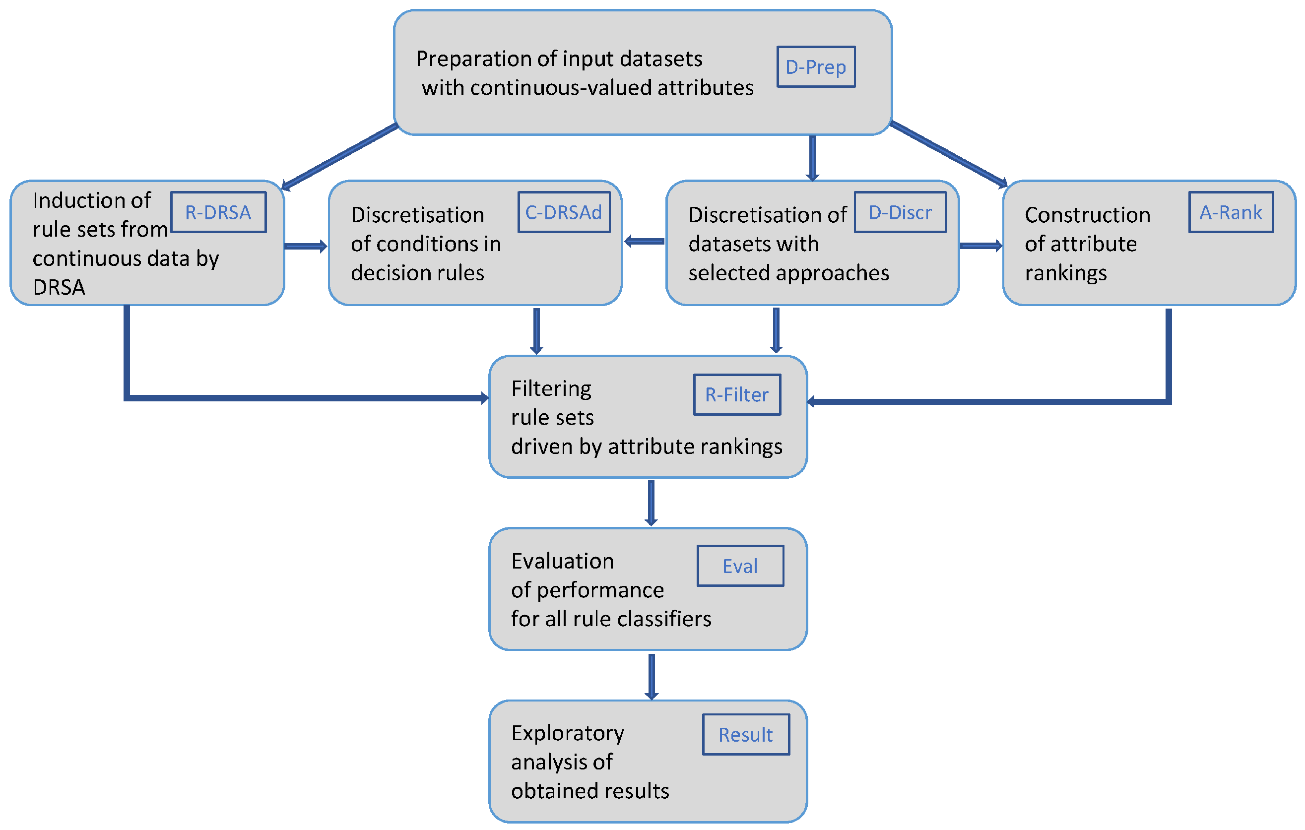
The research work described in this paper consisted of several stages, shown in Figure 1. It began with the selection of the application domain for the illustrative example. Once the input datasets were prepared for the experiments (D-Prep), they were explored with the Dominance-Based Rough Set Approach to find sets of decision rules (R-DRSA). For DRSA data mining, 4eMka2 Software was used, developed at Poznań University of Technology [42]. Then, both the data (D-Discr) and the knowledge patterns discovered and represented by the decision rules (C-DRSAd) were discretised by applying some algorithms available in the Waikato Environment for Knowledge Analysis (WEKA workbench) [43]. In the next stage, the sets of rules were filtered (R-Filter) by referring to rankings of attributes found for all data variants, continuous and discrete (A-Rank). For all constructed rule-based classifiers, performance was evaluated (Eval) and then analysed (Result). This subsection details the extent and conditions of the experiments that were carried out, while the results are given in the next section.

2.6.1. Application Domain of Stylometry

Stylometry aims at the impossible: measuring something as subtle and vague as a writing style and expressing it in quantitative terms [44]. Accepting that this ideal cannot be reached, approximations are sought, and writer profiles are constructed by explorative analysis of texts of known authorship to discover linguistic patterns. The task of authorship attribution is considered the most important in this application domain. It combines elements of other problems: author characterisation and author comparison. When profiles are first learnt and then compared against characteristics detected for text samples of unknown or questioned authorship, the attribution is treated as a classification, with stylometric markers playing the role of characteristic features, and recognised authors used as class labels.

Two datasets were prepared for the experiments, both dedicated to binary authorship attribution, and well-known writers of classical literature as considered authors [45]. The female writer dataset (F-writers) reflected the profiles of Edith Wharton and Mary Johnston, while the male writer dataset (M-writers) was focused on works by Jack London and James Oliver Curwood. Each dataset consisted of one training set and two test sets, including samples based on text blocks, found by partitioning long literary works into smaller chunks of comparable size. Samples obtained through the division and processing of one longer text (such as a novel) show a closer similarity. The way of textual data preparation leads to a space where not only classes are recognised but also hidden stratification of subclasses exists, imposed by groups of samples based on the same longer works.

Various sets of features can be used in stylometric analysis. More reliable are markers that are less likely to be imitated because they belong to linguistic elements used rather subconsciously, habitually, such as common function words [46], or they appear in text due to individual preferences or learnt traits, such as patterns of sentence formulation indicated by punctuation marks [47]. When the frequency of occurrence for these lexical and syntactic markers is calculated, the resulting values of the attributes are continuous.

In the investigations reported in this paper, the set of 24 features (22 lexical and two syntactic) was used. They are listed in

Table 1. Stylometric attributes and short symbols assigned to them.

Sym	Attr	Sym	Attr	Sym	Attr	Sym	Attr	Sym	Attr	Sym	Attr
a1	that	a5	what	a9	then	a13	same	a17	though	a21	around
a2	on	a6	who	a10	any	a14	such	a18	until	a22	within
a3	but	a7	there	a11	after	a15	during	a19	almost	a23	;
a4	by	a8	how	a12	never	a16	before	a20	whether	a24	,

with short symbols assigned to make presentation simpler. For both datasets, the same attributes were employed for analysis. To avoid problems connected with learning from imbalanced data, in all sets (training sets and test sets), both authors were represented by the same number of samples and also with the same hidden stratification structures.

2.6.2. Discretisation Approaches Used

To transform the input space, the representatives of both supervised and unsupervised discretisation algorithms were applied. From the former category, the Kononenko method was used [13]. In addition to that, unsupervised equal-width binning and equal-frequency binning were employed [4]. The Kononenko approach is non-parametric, but for the unsupervised procedures, the input parameter needs to provide the required number of bins to be defined for all attributes. This number ranged from two to ten. Therefore, the total number of variants of representation of the training data was equal to 20: one continuous, one for Kononenko discretisation (denoted dsK), nine for equal width, and nine for equal-frequency binning (denoted, respectively, duwi and dufi, with i giving the number of bins).

In the case of test sets, the number of discrete variants was doubled. Each test set was transformed independently on other sets (denoted Test independent, Tind), but also dependently. The observed values were then replaced with the corresponding categorical representation found in transformation of the training data (denoted Test on Learnt, ToL).

2.6.3. Stylometric Features and Rankings

Any transformation of the space also makes changes in dependencies and characteristics that can be detected. To account for this, an evaluation of the relevance of stylometric features was performed for all data variants explored, in the original continuous and all discrete domains investigated. The attributes were ranked with the help of the One Rule (OneR) algorithm [48]. It is based on the properties of the decision rules. In the procedure, short rules are constructed using attribute values for conditions, and performance serves as the weighting factor. The rankings obtained for all domains are listed in

Table 2. OneR rankings of attributes based on all data variants studied.

			Unsupervised Equal Frequency (dufi) Binning with i Bins									Unsupervised Equal Width (duwi) Binning with i Bins
R	Real	dsK	duf2	duf3	duf4	duf5	duf6	duf7	duf8	duf9	duf10	duw2	duw3	duw4	duw5	duw6	duw7	duw8	duw9	duw10
Female writer dataset
1	a24	a24	a24	a18	a24	a24	a24	a24	a24	a24	a24	a24	a24	a24	a24	a24	a24	a24	a24	a24
2	a18	a2	a2	a2	a2	a2	a2	a2	a2	a18	a2	a2	a2	a14	a2	a2	a2	a2	a2	a2
3	a2	a18	a18	a24	a18	a18	a18	a18	a18	a2	a18	a3	a23	a2	a23	a18	a18	a18	a18	a18
4	a23	a23	a23	a21	a23	a14	a23	a21	a23	a3	a23	a23	a7	a3	a14	a21	a14	a23	a14	a23
5	a21	a21	a14	a3	a14	a21	a21	a3	a21	a21	a21	a7	a14	a9	a3	a3	a21	a14	a21	a21
6	a14	a3	a21	a14	a21	a3	a3	a14	a3	a14	a3	a5	a3	a5	a7	a23	a3	a21	a3	a14
7	a7	a14	a3	a7	a3	a7	a7	a23	a14	a23	a9	a10	a5	a18	a21	a7	a23	a7	a23	a3
8	a3	a7	a7	a9	a7	a23	a14	a9	a9	a9	a7	a14	a10	a4	a18	a14	a7	a3	a5	a9
9	a13	a9	a9	a10	a9	a9	a9	a5	a7	a11	a14	a9	a9	a11	a9	a5	a9	a9	a7	a7
10	a9	a10	a5	a5	a5	a5	a13	a7	a5	a5	a5	a12	a18	a10	a10	a10	a10	a5	a10	a5
11	a22	a5	a10	a23	a13	a4	a8	a4	a8	a10	a10	a1	a8	a8	a11	a8	a5	a10	a8	a10
12	a5	a13	a11	a4	a8	a8	a5	a13	a4	a13	a13	a11	a11	a23	a13	a4	a13	a8	a13	a13
13	a8	a4	a4	a8	a22	a10	a4	a8	a13	a4	a4	a18	a13	a13	a4	a13	a8	a4	a4	a8
14	a6	a8	a13	a22	a19	a13	a1	a17	a22	a7	a8	a16	a6	a17	a5	a9	a1	a22	a9	a22
15	a17	a11	a22	a11	a17	a22	a10	a10	a15	a1	a22	a13	a19	a6	a17	a22	a22	a12	a22	a4
16	a15	a22	a19	a6	a11	a11	a17	a22	a10	a22	a15	a19	a17	a7	a22	a11	a16	a16	a17	a17
17	a12	a16	a17	a16	a16	a15	a22	a19	a19	a17	a17	a17	a16	a16	a12	a16	a4	a17	a12	a12
18	a10	a12	a1	a15	a4	a6	a15	a15	a11	a8	a19	a8	a12	a19	a1	a17	a6	a13	a15	a11
19	a19	a15	a6	a19	a15	a19	a11	a1	a17	a15	a11	a6	a21	a21	a19	a12	a11	a11	a11	a6
20	a11	a17	a15	a13	a12	a16	a16	a6	a6	a19	a1	a20	a1	a22	a8	a6	a15	a15	a6	a15
21	a1	a1	a16	a17	a6	a1	a12	a11	a16	a12	a12	a22	a22	a12	a16	a15	a12	a19	a19	a19
22	a20	a20	a8	a12	a1	a17	a6	a12	a20	a16	a20	a21	a4	a20	a20	a19	a19	a20	a16	a20
23	a16	a6	a12	a1	a20	a12	a19	a16	a1	a20	a16	a15	a20	a1	a6	a20	a20	a6	a1	a16
24	a4	a19	a20	a20	a10	a20	a20	a20	a12	a6	a6	a4	a15	a15	a15	a1	a17	a1	a20	a1
Male writer dataset
1	a24	a24	a24	a24	a24	a24	a24	a24	a24	a24	a24	a24	a24	a24	a24	a24	a24	a24	a24	a24
2	a18	a18	a18	a7	a18	a2	a18	a18	a18	a4	a4	a3	a4	a18	a18	a18	a18	a18	a18	a18
3	a17	a4	a4	a17	a4	a10	a4	a4	a4	a2	a18	a1	a18	a7	a2	a4	a7	a2	a4	a4
4	a7	a7	a7	a3	a2	a4	a2	a2	a2	a10	a14	a2	a7	a17	a4	a17	a4	a7	a17	a2
5	a4	a2	a2	a19	a7	a14	a7	a17	a17	a14	a2	a18	a2	a4	a17	a7	a2	a4	a7	a17
6	a3	a17	a14	a2	a1	a7	a14	a14	a14	a18	a1	a4	a19	a3	a19	a3	a19	a17	a19	a7
7	a10	a14	a3	a14	a19	a18	a1	a10	a7	a7	a7	a7	a10	a1	a3	a1	a3	a1	a3	a10
8	a19	a3	a1	a10	a3	a3	a10	a19	a1	a17	a17	a9	a3	a19	a14	a2	a17	a19	a10	a1
9	a14	a1	a17	a18	a17	a19	a19	a7	a3	a1	a9	a10	a9	a10	a1	a19	a10	a10	a1	a19
10	a2	a19	a19	a8	a8	a1	a3	a9	a10	a19	a10	a19	a6	a2	a7	a10	a14	a14	a2	a3
11	a8	a10	a10	a1	a14	a23	a8	a3	a9	a3	a3	a12	a17	a9	a9	a14	a9	a3	a14	a14
12	a9	a8	a13	a9	a10	a9	a17	a23	a8	a9	a19	a6	a14	a6	a21	a8	a6	a9	a23	a23
13	a1	a9	a6	a23	a16	a17	a13	a1	a23	a22	a23	a21	a16	a5	a6	a5	a8	a13	a13	a16
14	a22	a13	a8	a13	a6	a22	a22	a21	a16	a8	a22	a17	a21	a14	a8	a22	a22	a22	a9	a21
15	a21	a23	a22	a5	a5	a8	a16	a8	a19	a6	a21	a8	a20	a20	a5	a21	a16	a23	a22	a13
16	a15	a5	a9	a4	a11	a6	a21	a22	a22	a15	a16	a11	a5	a21	a22	a6	a21	a8	a21	a22
17	a23	a6	a21	a21	a22	a5	a5	a16	a6	a16	a8	a5	a1	a13	a10	a9	a1	a21	a16	a5
18	a20	a21	a23	a6	a21	a13	a23	a15	a15	a21	a12	a14	a22	a22	a13	a15	a15	a6	a15	a6
19	a16	a22	a11	a16	a23	a15	a11	a20	a5	a20	a15	a23	a8	a12	a23	a13	a23	a15	a8	a8
20	a5	a16	a15	a15	a15	a21	a15	a6	a13	a23	a20	a13	a12	a11	a20	a23	a13	a5	a5	a9
21	a13	a20	a20	a22	a20	a20	a6	a5	a21	a13	a6	a16	a13	a23	a15	a16	a20	a20	a6	a15
22	a11	a11	a5	a20	a13	a16	a9	a13	a20	a5	a11	a20	a11	a8	a12	a20	a5	a12	a20	a20
23	a12	a12	a12	a12	a9	a11	a20	a12	a11	a11	a5	a15	a23	a16	a11	a12	a12	a11	a12	a12
24	a6	a15	a16	a11	a12	a12	a12	a11	a12	a12	a13	a22	a15	a15	a16	a11	a11	a16	a11	a11

Column R provides a ranking position detected in the continuous (Real) and discrete domains, supervised Kononenko (dsK), and unsupervised equal-frequency (duf) and equal-width (duw) binning. The colour scale of the heat map is based on the ranking in the continuous domain given in the column Real. Colour scales are based on the rankings in the continuous domain, to show how relevance is affected by discretisation. The deepest blue reflects the highest ranking variables, and the deepest red the least important attributes.

, where the column R provides a ranking position for all domains studied, from 1 (top) to 24 (bottom).

The form of a heat map adopted to simplify presentation relies on colour scales based on the rankings in the original continuous domain to visualise the effects of discretisation. They are mostly different between the two datasets, that is, similarities (when the same colour is used for the same attribute for both datasets) occurred only when some variables were ranked in the same way. The variables placed at the top, which means that they are considered the most important, were shown with a blue gradation, fading to white in the middle ranges of relevance, and then changing to deeper shades of red for the least important features.

With a single exception, both datasets agreed with respect to the attribute found as the most important for all data variants: it was a24 (comma). Only for the female writer dataset transformed with the duf3 approach was the highest ranked variable a18 (until). There were also cases where an attribute was relatively more important in the continuous domain, but after discretisation, its relevance was noticeably changed, either lower or higher, for example, for F-writers, a21 (around) in the duw2 approach or a4 (by) and the duf5 approach, and for M-writers, again a4 and duf3, or a6 (who) and the duw3 discretisation. Generally, higher degrees of similarity could be observed between rankings resulting from some variants of the same unsupervised discretisation algorithms, but no two rankings were the same. All rankings were employed to drive the rule filtering process.

2.6.4. Procedure of Ranking-Driven Rule Filtering

The rule filtering procedure (with the pseudo-code given by Algorithm 1) was executed iteratively, with the number of iteration steps equal to the number of attributes available. Each step involved considerations on one attribute. The order in which the variables were selected was determined by the rankings investigated but could be driven by any defined ordering. In the continuous domain, one ranking was studied, obtained for the original input training sets. In each discrete domain, in addition to this ranking based on the input data, the ranking calculated for this particular discrete data variant was also applied in rule filtering to examine the influence of both the original and transformed data on the process.

Two directions of the search procedure were used: forward and backward. For the forward direction, the starting point was the empty set to which rules were gradually added by referring to attributes listed by the ranking, beginning with the top positions. The stopping point was reached when the least important variable was selected and all induced rules were included in the recalled set. The backward search began at the bottom of the ranking, with the entire set of available rules, from which the elements were discarded in iteration steps, as indicated by gradually more and more important features. The procedure stopped when reaching the top of a ranking, when all attributes and rules were discarded.

Algorithm 1 Pseudo-code for rule filtering controlled by an ordering of attributes

Input: number of attributes M,             set of attributes Attrib,             ordering of attributes $Orde{r}_A$,             set of decision rules Rules,             search direction Direction to follow ordering of attributes OrderA; begin if Direction=Forward then             //initialisation              Attrib-TMP = $Ø$              Rules-TMP = $Ø$ else             Attrib-TMP = Attrib              Rules-TMP = Rules for i = 1 to $M$ do                              //process iteratively all $M$ attributes              if Direction=Forward then                           select attribute from the ordering attr = OrderA[i]  //select the variable                           Attrib-TMP = Attrib-TMP ∪ attr     //expand the set of variables                           Rules-TMP = SelectRules(Rules, Attrib-TMP)       //select the rules                                     including conditions on attributes limited to the selected subset             else                   select attribute from the ordering attr = OrderA[M − i + 1]                                       //select the variable                   Attrib-TMP = Attrib-TMP \attr                  //reduce the set of variables                   Rules-TMP = Rules-TMP \ SelectRules(Rules-TMP, Attrib \ Attrib-TMP)                                     //from the currently considered set of rules remove those with                                     conditions on attributes limited to the discarded subset endfor end {algorithm}

Different strategies of rule selection were assigned to the two investigated directions. For forward search, these rules were recalled, which in their premises included conditions on variables that belonged to the set of elements considered for each specific iteration step. In the first step, only rules with single conditions on the top ranking variables could be selected. In the second step, the recalled rules could have at most two conditions and refer to one or two top ranking features, and so on. In the backward search procedure, the rules were rejected when they did not include any condition on variables still remaining in considerations. Therefore, for the forward search, the iteration step also indicated the number of variables. For the backward search, it could not be interpreted in this way because still some rules could be present in the remaining set because the conditions were included on other, higher ranked attributes. In consequence of these two strategies, at the same iteration step, there could be a huge difference in the number of rules between the two directions.

Taking into account different rankings and directions, the rule filtering procedures examined were as follows.

• Real-Forward (RF)—Based on the ranking in the continuous domain, starting at the top, and gradually expanding the set of rules, applied in all domains;
• Real-Backward (RB)—Based on the ranking in the continuous domain, starting at the bottom, and with discarding rules with each iteration step, applied in all domains;
• Discrete-Forward (DF)—Based on a ranking in a specific discrete domain and used only in this domain, executed forward;
• Discrete-Backward (DB)—Based on a ranking in a specific discrete domain, applied only in this domain, and search performed backward.

To sum it up, for both female and male writer datasets in the continuous domain, two filtering procedures (RF and RB) were performed, while each discrete variant was subjected to four procedures (RF and RB, and DF and DB). This makes a total of 78 procedures per dataset studied taking into account several characteristics.

2.6.5. Evaluation of Performance

To evaluate the performance of rule-based classifiers, the measure of classification accuracy was selected. It specifies the percentage of correctly classified samples, regardless of class. This choice was made because of the working conditions of inducers [49]: the classification task was binary; the recognised classes were equally represented, so there was no imbalance; and both classes were of the same importance, with the same misclassification costs (false negative had the same meaning as false positive). The classification accuracy was calculated individually for the test sets used and then averaged. This average is the final elementary result given. In discrete domains, because of two modes of transformation adapted to test sets, independent and dependent, the evaluations and then calculated averages were studied for both.

The application of test sets in the evaluation, as opposed to some variant of a popular cross-validation technique [50] results from the characteristics of the input space studied, with hidden stratification formed by subclasses, which is the consequence of data preparation. In such conditions, cross-validation tends to return falsely over-optimistic evaluations. To make it more reliable would involve the selection of not just random samples, as per the standard, but groups of samples corresponding to entire subclasses [51]. This kind of processing was unfeasible because greatly extends the processing time and increases computational costs, which in the reported research, would be even greater due to multiple data variants examined and the relatively complex data exploration and then transformation. Using averages calculated over test sets provides a reasonable compromise and a sufficiently reliable estimation of accuracy.

3. Results

For all domains in which the input data were investigated, original continuous and all discrete variants, the process of rule filtering based on attribute rankings was executed. This section is focused on the observations of trends in the performance of the constructed rule-based classifiers, while characteristics of the rule filtering process performed under various conditions are discussed in the following.

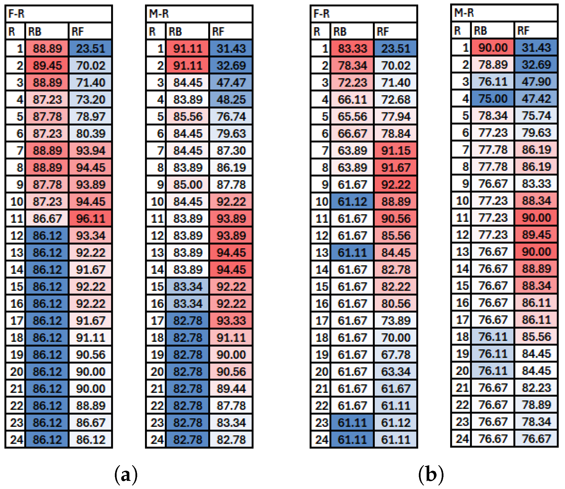
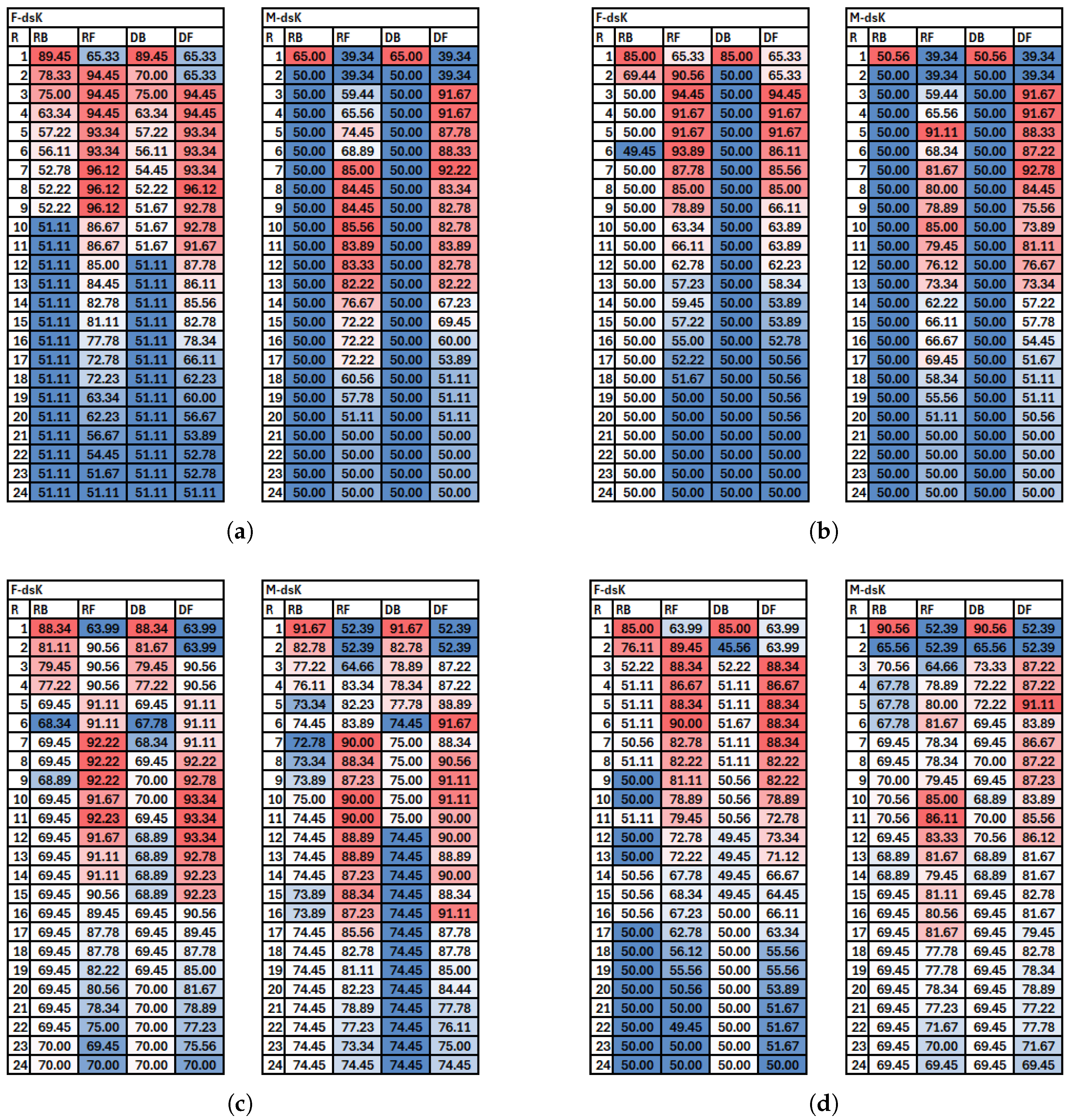
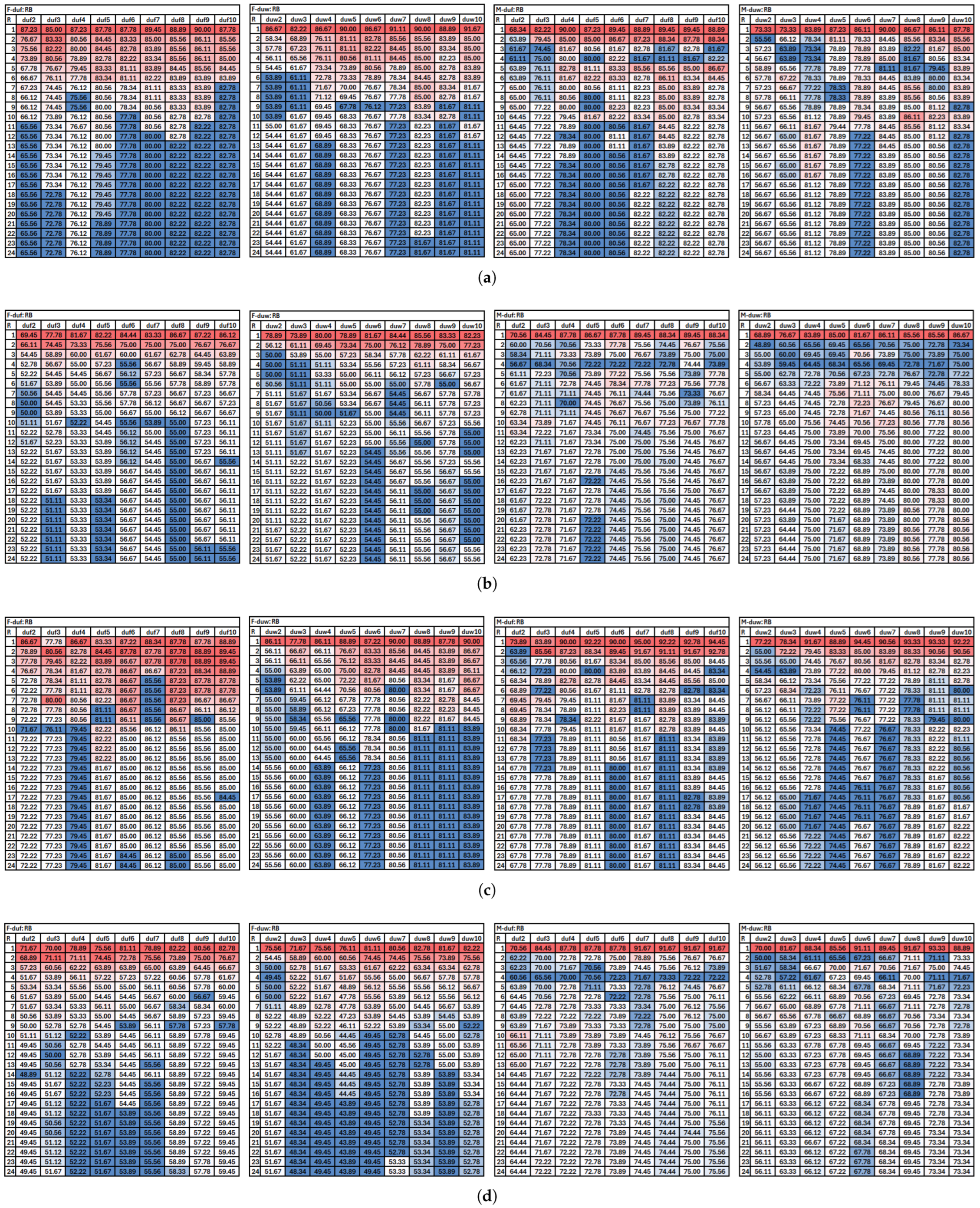
The performance of inducers, evaluated by the classification accuracy averaged over test sets, is shown in figures separately for the datasets and rule filtering procedure, for the two conflict resolving methods and modes of transformation applied for discretised test sets. Each filtering procedure adopts its own individual colouring scheme: the highest values are displayed with shades of red background, gradually becoming lighter until the middle range is reached, which is white, and then lower and lower predictions are given with darkening shades of blue. This form of heat map simplifies the detection of trends in performance and facilitates intuitive understanding of the presentation. The results marked as hot (red) correspond to higher values, while cold (blue) zones indicate lower predictions.

For all procedures, the entire path was examined, from zero attributes and rules to all attributes and rules, or the other way round. R corresponds to the ranking positions considered. For the forward search, it directly specifies the number of iteration steps currently processed and equals the number of features selected. This is not true for the backward search due to the different strategies in discarding rules and the starting point of all available rules. The value of the ranking position for R equal 24 denotes the entire set of induced rules available; therefore, the only difference between directions could happen for different types of voting in the case of existing conflicts.

3.1. Operation with All Rules

Exploration of the original input data in the continuous domain with DRSA for all rules on the example algorithm implemented in 4eMka2 Software returned the sets of decision rules for both datasets, with the characteristics listed in

Table 3. Characteristics of rule sets in the continuous domain.

		Length			Support					Accuracy
Dataset	NrR	Avg	Min	Max	Avg	Min	Max	ConfR	Cover	VS:W	VS:M
F-writers	23006	5.40	1	12	3.22	1	92	0.917	1	86.12	61.11
M–writers	40179	4.55	1	10	8.47	1	78	0.983	1	82.78	76.67

Columns list the number of rules NrR, characteristics of rule length and support: average Avg, minimum Min and maximum Max, conflict rate ConfR, coverage Cover, and classification accuracy [%] for each voting strategy VS (either weighted W voting or simple majority M voting).

. These two sets of decision rules provided the basis for all procedures and transformations directed at simplification, resulting in some improvement in the interpretability of decision making. The performance evaluated for these two sets, including all induced rules involved in labelling the test samples, constituted a reference point for comparison in the investigations.

For the female writer dataset, the difference in evaluation dependent on the conflict resolution strategy was noticeably larger, but for both datasets, weighted voting caused higher classification accuracy than simple majority voting. The two sets of decision rules provided perfect coverage of the test samples. The conflict rate was close to one due to the high number of rules. The numbers of rules which fired for a test sample varied but generally were in the range of several thousands. For both datasets, the minimum rule length was equal to one. It was also the minimal value of the rule support. The maximum length was higher for F-writers than for M-writers but so was the maximal value of support. Despite the lower number of rules; for the female writer dataset, the average support was lower; and the average rule length was larger than these two important characteristics of rules for the male writer dataset.

One of the approaches used in this research for the purpose of simplification of a decision-making process was discretisation. The transformation was applied both to the data and the patterns learnt from the data and then represented by the sets of decision rules. Discretisation of conditions included in rule premises returned sets with the same general characteristics such as the numbers of rules, their lengths, and supports, but the translation could cause different working conditions, that is, different conflict rates, coverage, and obviously the performance. These elements are given in

Table 4. Characteristics of rule sets in the discrete domains.

	Female Writer Dataset								Male Writer Dataset
	Tind Test Sets				ToL Test Sets				Tind Test Sets				ToL Test Sets
			Accuracy				Accuracy				Accuracy				Accuracy
Domain	ConfR	Cover	VS:W	VS:M	ConfR	Cover	VS:W	VS:M	ConfR	Cover	VS:W	VS:M	ConfR	Cover	VS:W	VS:M
dsK	1.000	1	51.11	50.00	1.000	1	70.00	50.00	1.000	1	50.00	50.00	1.000	1	74.45	69.45
duf2	1.000	1	65.56	52.22	1.000	1	72.22	49.45	1.000	1	65.00	62.23	1.000	1	67.78	64.44
duf3	1.000	1	72.78	51.11	1.000	1	77.23	51.67	1.000	1	77.22	72.78	1.000	1	77.78	72.22
duf4	0.994	1	76.12	53.33	0.994	1	79.45	52.22	1.000	1	78.34	71.67	1.000	1	78.89	72.22
duf5	0.983	1	78.89	53.34	1.000	1	81.67	51.67	1.000	1	80.00	72.22	1.000	1	81.11	72.78
duf6	0.983	1	77.78	56.67	0.994	1	84.45	53.89	1.000	1	80.56	74.45	1.000	1	80.00	73.89
duf7	0.967	1	80.00	54.45	0.989	1	86.12	55.56	0.994	1	82.22	75.56	1.000	1	81.67	74.45
duf8	0.972	1	82.22	55.00	0.994	1	85.00	58.33	0.994	1	82.22	75.00	1.000	1	81.11	74.44
duf9	0.972	1	82.22	56.11	0.983	1	85.56	57.78	0.994	1	82.22	74.45	1.000	1	83.34	75.00
duf10	0.961	1	82.78	55.56	0.978	1	85.00	59.45	0.994	1	82.78	76.67	1.000	1	84.45	75.56
duw2	1.000	1	54.44	51.67	1.000	1	55.56	51.67	1.000	1	56.67	57.23	1.000	1	56.12	56.11
duw3	1.000	1	61.67	52.22	1.000	1	60.00	48.34	1.000	1	65.56	64.44	1.000	1	65.56	63.33
duw4	1.000	1	68.89	51.67	1.000	1	63.89	49.45	1.000	1	81.12	75.00	1.000	1	72.22	66.12
duw5	1.000	1	68.33	52.23	1.000	1	66.12	43.89	1.000	1	78.89	71.67	1.000	1	74.45	67.22
duw6	1.000	1	76.67	54.45	1.000	1	77.23	49.45	1.000	1	77.22	68.89	1.000	1	76.67	67.78
duw7	1.000	1	77.23	56.11	1.000	1	80.56	53.33	1.000	1	83.89	73.89	1.000	1	76.67	68.34
duw8	1.000	1	81.67	55.56	0.994	1	81.11	53.34	1.000	1	85.00	80.56	1.000	1	78.89	69.45
duw9	1.000	1	81.67	56.67	0.994	1	81.11	53.89	1.000	1	80.56	77.78	0.994	1	81.67	73.34
duw10	1.000	1	81.11	55.56	0.994	1	83.89	52.78	1.000	1	82.78	80.56	0.994	1	82.22	73.34

Columns list conflict rate ConfR, coverage Cover, and classification accuracy [%] for each voting strategy VS (either weighted W voting or simple majority M voting) and evaluation by test sets processed independently (Tind) or dependently (ToL).

. Due to the two considered processing modes adopted for the test sets, dependent and independent, the characteristics related to performance evaluation were listed separately for both types of test sets.

In all discrete domains, the complete sets of rules provided coverage for all test samples, regardless of the transformation mode adapted for the test sets. Although for the majority of cases, the conflict rate was equal to one, there were some exceptions to this rule. For the female writer dataset, they occurred for the Tind and discrete domains obtained by unsupervised equal-frequency binning with the number of bins from four to ten, and for the ToL test sets for both unsupervised discretisation approaches, from duf4 to duf10 and from duw8 to duw10. For M-writers, slightly different patterns emerged: for the Tind test sets, the fractional conflict rate was observed for equal-frequency binning with bins ranging from seven to ten, and for the ToL test sets, the same was detected for equal-width binning with nine or ten bins.

A comparison of performance within the voting strategy resulted in the conclusion that for F-writers and weighted voting, the reference point was reached in the duf7 domain for evaluation with dependently transformed test sets, while for all other conditions, the accuracy was lower than in the continuous domain. In this case, the majority voting always fell below the reference point for both types of test sets. On the other hand, some improved accuracy was recorded for M-writers. For the Tind test sets, both for weighted and simple majority voting applied when conflicts occurred, the performance was better in the duw7 and duw8 domains for the former and in the duw8 and duw10 domains for the latter, and for the ToL test sets in the duf9 and duf10 domains for weighted voting.

The discretisation process returned a more general form of definitions for knowledge patterns discovered, which can be considered beneficial because the risk of overfitting the input data reduced. Transformations affected performance and not necessarily to an advantage. The high numbers of inferred rules reflected on the high values of the conflict rate and suggested that an exploratory analysis of rules and rule filtering can lead to dimensionality reduction and possible improvements. The characteristics of decision making with rule sets subjected to filtering driven by attribute rankings were then studied.

3.2. Operation with Rule Filtering

When rule-based classifiers operated in the continuous domain, only one ranking was used as the ordering controlling the rule filtering procedure, based on real-valued attributes, executed in two directions: forward (RF) and backward (RB). Only one type of test set was employed in the performance evaluation, with two voting strategies resolving conflicts, weighted voting, and simple majority voting. Together, this accounts for four sets of results obtained for each dataset, the female writer dataset (denoted F-R) and the male writer dataset (denoted M-R), with R giving the iteration steps, as displayed in Figure 2.

An analysis of patterns of predictions leads to the observation of similarities for both datasets using the same voting strategy but also for processing in the same direction. For the backward search, in the initial steps of discarding rules, the performance was never the best, at most in the middle ranges. Only once sufficiently many rules were rejected did the accuracy improve, with the highest values close to or at the very end of the rule filtering process. In the forward search procedure, the initial iteration steps retrieved relatively few rules, which caused rather poor recognition that was enhanced with more and more rules recalled, but when they became too numerous, the performance degraded. For this direction, the best results could be observed somewhere around the half-way point of the processing path.

Generally, weighted voting was more advantageous to reported performance than simple majority voting, but the differences were more noticeable when more rules were used in the classification. Higher numbers of rules meant that more of them could have lower supports, but by their sheer number, they outvoted stronger rules that were less numerous. For relatively low cardinalities of rule sets, such as recalled in the initial steps of a forward search, the accuracy was either the same or very close for both types of voting. The same was not necessarily true for the ending steps of the backward search, which by the different strategy of retaining rules, caused more of them to be employed in processing until the very last step of filtering.

For all procedures of rule filtering, some improvement over the performance for the entire set of available rules was detected, occurring for noticeably lower numbers of rules. Therefore, this part of the research alone already shows the merits of the adopted methodology. However, the gains were limited mainly to the dimensionality expressed by the cardinalities of the rule sets and their characteristics, while the constituent elementary rules remained unchanged. As a way to modify them further, the translation into discrete domains was also studied in the context of rule filtering.

Each discrete domain was characterised by its own ranking of features, which doubled the number of processing paths. In addition to that, two modes of transformation applied to test sets further doubled the number of performance evaluations and sets of results listed. Therefore, in each domain, the total of 16 groups of records, corresponding to 24 iteration steps, were taken per dataset and studied in categories of voting type and test set type.

Figure 3 includes the results for the discrete domain obtained by application of the supervised Kononenko algorithm (denoted dsK and, respectively, F-dsK and M-dsK) for all four processing paths. Since this discretisation method is supervised and relies on the process of forming intervals on the evaluation of how attributes support the distinction of classes, it can in effect remove some of features from consideration in the discrete space when a single bin is assigned to represent the entire domain. This was the case with the datasets explored. For independent transformations of test sets, different variables were found as single-bin variables due to irregularities in the data, which resulted in generally much degraded performance reported for evaluation with the Tind test sets and entire sets of rules applied in labelling. The ToL test sets, for which discretisation procedures rely on the intervals learnt from the training data, led to better results for both datasets in the case of weighted voting as the conflict resolution strategy, but for simple majority voting only for the male writer datasets, while for F-writers, still, poor accuracy was recorded.

Because of the similarities between rankings in the continuous and discrete dsK domain, also trends in performance were close when filtering was executed in the same direction, but with control by the two different rankings. For backward search, there were fewer or smaller differences. For M-writers, identical evaluations were obtained with the Tind test sets at all steps for the RB and DB procedures with weighted and majority voting. For forward processing, more variations could be detected for both datasets.

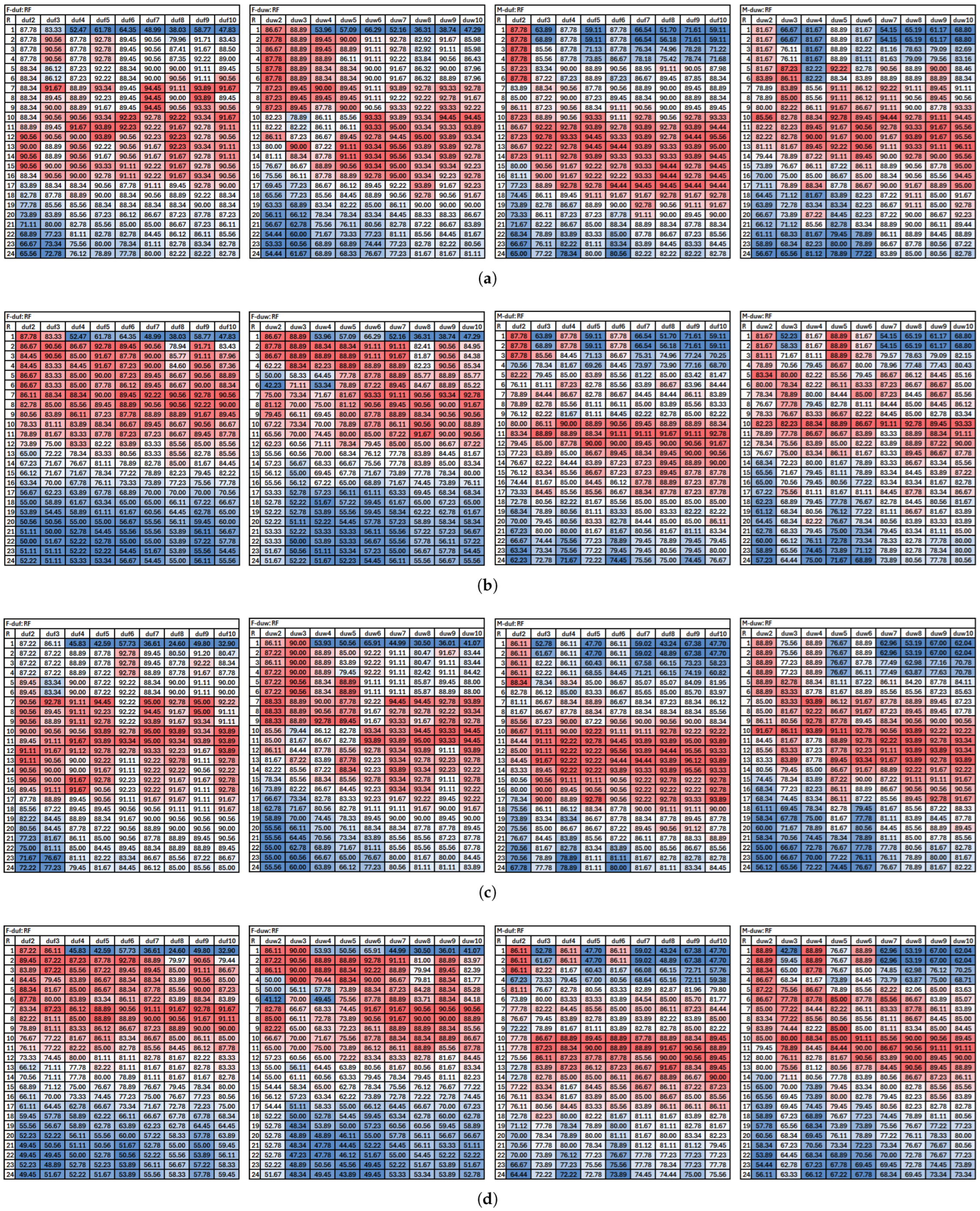
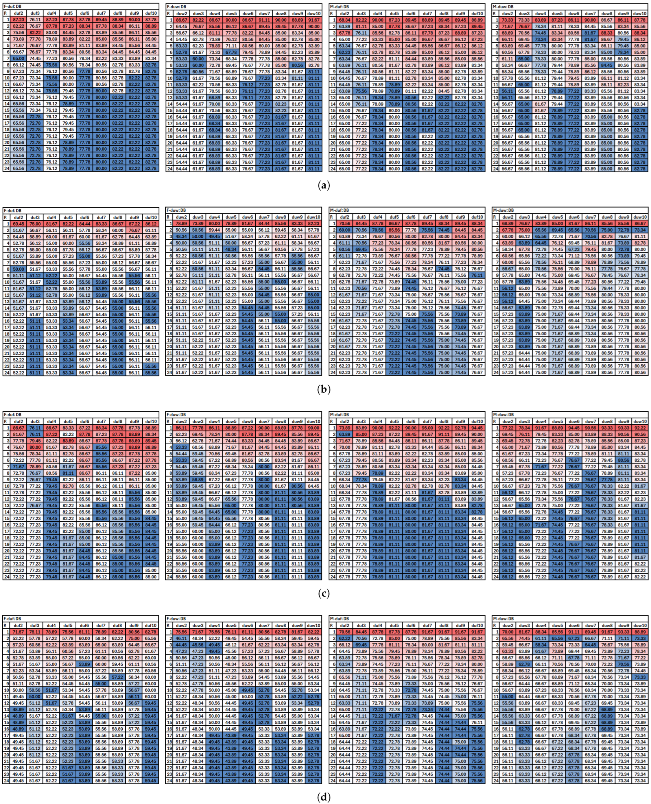
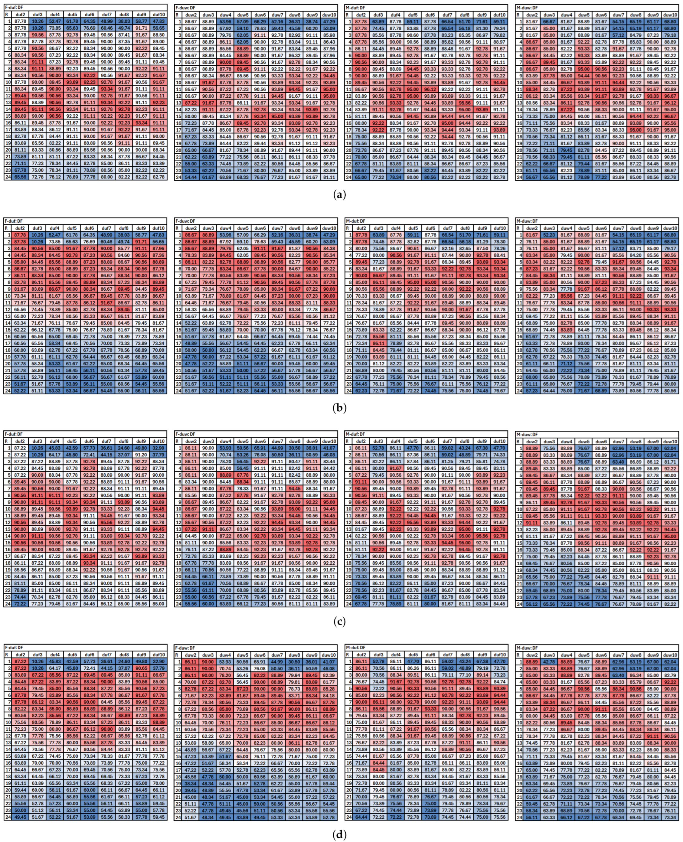
Each of the two unsupervised discretisation methods used in the research, equal width binning (duw) and equal frequency binning (duf), returned nine data variants due to ranging the number of bins from two to ten. For this kind of transformation, for all attributes processed, the required intervals were formed, so no attributes were removed from considerations as a consequence of the changed representation. Both independently and dependently transformed test sets had the same numbers of intervals defined for the variables, but they were not the same because of different cutpoints, which also in this case resulted in differently evaluated accuracy. To allow for closer observations of trends for all discrete data variants, for each filtering procedure characterised by direction and source of ranking, the performance of rule-based classifiers was shown separately by Figure A1, Figure A2, Figure A3 and Figure A4 included and commented on in the Appendix A.

When rule filtering was based on the rankings obtained for each of the discrete data variants considered, it was reasonable to expect that for both forward and backward directions of processing, more differences in the effectiveness of rule-based classifiers constructed should be visible than when one ranking led the way. However, because of similarities between the rankings, these intuitive expectations were not fully confirmed by the experimental results. Some different patterns and trends were observed, but not so striking as to form a contrast with the accuracy evaluations for the RF and RB procedures. Furthermore, the experimental results do not confirm the superiority of supervised methods over unsupervised algorithms used in discretisation. For the same filtering procedure (the same direction and ranking), the Kononenko method did not cause the representation of attributes to be more beneficial to performance evaluation than unsupervised approaches.

For all procedures, rule filtering proved to be effective because it led to acceptable levels of correct predictions. The patterns of accuracy were similar to those observed in the continuous domain. With some variations around the trends, backward search showed improvement with more and more rejected rules, even to the point of the maximum at the very end, at the last iteration step. Forward selection brought a gradual increase in performance, but then, with more retrieved rules, this was followed by a decrease. Not all processing paths and evaluation ways reached the same level as the maximum detected while filtering rules with conditions on numerical variables, but always some subset of rules worked better than the reference point in the continuous domain, that is, working with the entire set of decision rules.

For all domains and all procedures, basic statistics were calculated, including classification accuracy averaged over all processing steps and standard deviation associated with it. The extrema, maximum and minimum, were also detected. These elements are given in the included tables, in which the preferred best results are marked in bold font.

Table 5. Characteristics of performance for rule filtering processes executed in the continuous domain.

	Female Writer Dataset				Male Writer Dataset
	Direction: RB		Direction: RF		Direction: RB		Direction: RF
	VS:W	VS:M	VS:W	VS:M	VS:W	VS:M	VS:W	VS:M
Avg	87.02	64.35	85.29	74.35	84.28	77.41	80.80	77.01
Std	1.18	5.73	15.18	15.17	2.25	2.80	19.50	17.76
Min	86.12	61.11	23.51	23.51	82.78	75.00	31.43	31.43
Max	89.45	83.33	96.11	92.22	91.11	90.00	94.45	90.00

Rows list average Avg, standard deviation Std, and minimum Min and maximum Max classification accuracy [%] for each voting strategy VS (either weighted W voting or simple majority M voting). The preferred best values are marked with bold font.

describes the operation in the continuous domain, where all procedures are shown together for both female and male writer datasets. Due to the different strategy of rule selection associated with processing directions, for the backward search, noticeably lower standard deviation values showed a much smaller range of recorded accuracy in the iteration steps than for the forward search. On the other hand, it was the latter approach that led to the best performance found in the evaluation with weighted voting in the case of occurring conflicts for both datasets.

For discrete domains, due to twice as many filtering procedures, the characteristics were grouped into tables by the specifics of the procedure.

Table 6. Characteristics of performance for rule filtering processes executed backwards in discrete domains based on ranking in the continuous domain.

	Domain
	dsK	duf2	duf3	duf4	duf5	duf6	duf7	duf8	duf9	duf10	duw2	duw3	duw4	duw5	duw6	duw7	duw8	duw9	duw10	VS	Test
Female writer dataset
Avg	55.97	67.96	75.16	77.23	80.83	79.17	81.32	83.29	83.47	83.42	56.06	63.12	71.18	71.34	77.99	78.96	83.43	82.41	82.36	W	Ind
Std.	10.28	5.25	3.68	2.56	2.30	2.57	2.30	1.65	1.99	1.31	6.61	4.52	4.14	5.85	2.69	3.61	1.92	1.54	2.43
Min	51.11	65.56	72.78	75.56	78.89	77.78	80.00	82.22	82.22	82.78	53.89	61.11	68.89	67.78	76.12	77.23	81.67	81.67	81.11
Max	89.45	87.23	85.00	87.23	87.78	87.78	89.45	88.89	90.00	87.78	86.67	82.22	86.67	90.00	86.67	91.11	90.00	88.89	91.67
Avg	52.25	53.29	54.65	55.81	56.69	58.57	57.27	58.01	59.44	58.82	52.50	53.24	53.61	54.77	57.01	57.99	58.50	59.05	57.99	M	Ind
Std.	8.03	4.58	6.92	6.94	7.15	6.72	7.05	7.46	7.30	7.29	5.74	4.82	6.75	6.74	6.71	7.02	7.59	6.41	6.90
Min	49.45	50.00	51.11	52.22	53.34	55.56	53.89	55.00	56.11	55.56	50.00	51.11	50.00	51.67	54.45	54.45	55.00	55.00	55.00
Max	85.00	69.45	77.78	81.67	82.22	84.44	83.33	86.67	87.22	86.12	78.89	73.89	80.00	78.89	81.67	84.44	85.56	83.33	82.23
Avg	71.44	73.56	77.69	80.37	82.15	85.65	86.25	86.18	86.27	86.04	56.55	61.41	65.56	68.78	78.94	81.41	82.20	81.92	84.77	W	ToL
Std.	4.94	3.37	1.00	1.68	0.82	0.96	0.72	0.93	1.22	1.67	6.32	4.04	4.47	5.52	2.72	2.36	1.86	1.57	1.55
Min	68.34	71.6	76.11	79.45	81.11	84.45	85.56	85.00	85.00	84.45	53.89	58.34	63.89	65.56	77.23	80.00	81.11	81.11	83.89
Max	88.34	86.67	80.56	86.67	84.45	87.78	88.34	87.78	88.89	89.45	86.11	77.78	86.11	88.89	87.22	90.00	88.89	87.78	90.00
Avg	52.96	52.06	53.66	55.14	55.51	56.69	58.10	60.79	59.37	61.51	52.57	50.51	51.81	47.66	53.59	55.74	56.46	56.97	56.16	M	ToL
Std.	8.62	5.91	5.63	6.60	6.58	6.68	6.21	5.58	5.91	5.90	5.00	5.14	5.55	7.23	8.16	7.05	7.39	6.82	7.43
Min	50.00	48.89	50.00	52.22	51.67	53.89	55.56	57.78	56.67	57.78	49.45	48.34	49.45	43.89	49.45	52.78	52.78	53.89	52.22
Max	85.00	71.67	71.11	78.89	75.56	81.11	78.89	82.22	80.56	82.78	75.56	71.67	75.56	76.11	81.11	80.56	82.78	81.67	82.22
Male writer dataset
Avg	50.63	64.54	77.13	79.98	80.76	81.76	82.75	83.84	83.12	83.47	57.57	65.86	79.96	79.30	78.15	84.21	84.77	81.00	83.45	W	Ind
Std.	3.06	1.29	1.43	2.74	1.78	2.17	1.84	2.10	1.87	1.83	3.41	1.74	2.61	1.76	1.85	1.41	1.24	1.33	1.19
Min	50.00	61.11	74.45	78.34	80.00	80.56	81.67	81.11	81.67	81.67	55.56	63.89	73.34	78.33	77.22	81.11	81.67	79.45	82.78
Max	65.00	68.34	82.22	90.00	87.23	89.45	88.89	89.45	89.45	88.89	73.33	73.33	83.89	87.23	86.11	90.00	86.67	86.11	87.78
Avg	50.02	62.02	72.34	72.20	73.70	75.76	76.06	75.81	75.30	77.06	56.95	64.21	74.05	72.73	69.72	74.70	79.49	76.92	79.54	M	Ind
Std.	0.11	2.33	2.80	3.39	2.89	2.89	3.02	2.81	3.10	2.54	3.15	3.05	3.63	3.08	3.01	2.93	2.47	2.67	2.53
Min	50.00	56.67	68.34	70.00	72.22	72.22	72.22	72.78	73.33	73.89	48.89	59.45	64.45	68.34	65.56	69.45	72.78	71.67	73.34
Max	50.56	70.56	84.45	87.78	86.67	87.78	89.45	88.34	89.45	88.34	68.89	76.67	83.89	85.00	81.67	86.11	85.56	85.56	86.67
Avg	75.49	68.01	78.38	80.07	81.99	81.71	82.94	82.89	84.33	84.98	57.02	66.37	73.70	76.02	77.96	77.98	79.81	82.57	82.24	W	ToL
Std.	3.94	1.72	2.04	2.82	2.66	2.80	3.36	3.04	2.52	2.70	4.36	2.98	4.14	3.37	4.03	3.21	3.63	3.00	2.96
Min	72.78	63.89	77.22	78.34	80.00	80.00	81.11	81.11	82.78	83.34	54.45	63.89	71.67	74.45	76.11	76.67	77.78	79.45	80.00
Max	91.67	73.89	85.56	90.00	92.22	90.00	95.00	92.22	92.78	94.45	77.22	78.34	91.67	88.89	94.45	90.56	93.33	93.33	92.22
Avg	70.07	64.44	71.74	73.03	73.26	74.00	74.79	75.58	75.83	76.34	55.81	63.49	67.22	68.36	70.00	68.43	70.69	73.59	73.94	M	ToL
Std.	4.49	1.72	3.04	3.22	3.20	3.00	3.83	3.49	3.48	3.40	3.46	4.36	4.80	3.76	4.65	4.58	4.54	4.28	3.23
Min	65.56	60.56	65.56	70.00	70.56	72.22	71.67	73.33	72.22	72.22	50.00	57.22	61.11	65.56	67.23	66.11	68.89	71.11	71.67
Max	90.56	70.56	84.45	87.78	87.78	87.78	91.67	91.67	91.67	91.67	70.00	81.67	88.34	85.56	91.11	89.45	91.67	93.33	88.89

Rows list average Avg, standard deviation Std, and minimum Min and maximum Max classification accuracy [%] for each voting strategy VS (either weighted W voting or simple majority M voting) and evaluation by test sets processed independently (Test: Ind) or dependently (Test: ToL). For each domain, the preferred best values are marked with bold font.

corresponds to the filtering with backward search and control provided by the ranking in the continuous domain for all variants of discrete data. The results for the same ranking but for the forward direction of rule selection are given in

Table 7. Characteristics of performance for rule filtering processes executed forward in discrete domains based on ranking in the continuous domain.

	Domain
	dsK	duf2	duf3	duf4	duf5	duf6	duf7	duf8	duf9	duf10	duw2	duw3	duw4	duw5	duw6	duw7	duw8	duw9	duw10	VS	Test
Female writer dataset
Avg	78.86	83.77	86.51	85.61	89.01	87.10	88.18	86.67	89.60	87.01	75.97	80.65	83.13	83.67	87.51	88.70	87.23	88.37	87.43	W	Ind
Std.	15.65	8.22	5.48	8.24	7.22	6.13	9.20	10.89	7.33	8.78	13.03	11.00	9.05	8.88	7.32	9.62	11.71	11.17	9.56
Min	51.11	65.56	72.78	52.47	61.78	64.35	48.99	38.03	58.77	47.83	53.33	60.00	53.96	57.09	66.29	52.16	36.31	38.74	47.29
Max	96.12	90.56	91.67	91.67	93.89	92.23	94.45	92.23	93.89	91.67	87.78	90.00	90.00	91.11	93.34	95.56	95.00	94.45	94.45
Avg	66.84	69.98	71.87	72.23	75.81	75.41	75.70	74.70	77.43	76.27	62.13	64.17	65.12	69.30	74.61	74.74	74.70	76.45	75.54	M	Ind
Std.	17.14	14.49	14.41	14.02	15.04	13.31	15.51	15.46	14.48	14.23	13.43	13.54	11.80	13.11	14.11	14.94	15.02	15.89	14.58
Min	50.00	50.00	50.00	52.22	52.22	54.45	48.99	38.03	55.56	47.83	42.23	50.00	51.11	52.23	54.45	52.16	36.31	38.74	47.29
Max	94.45	87.78	90.56	88.34	92.78	89.45	92.22	90.56	92.78	90.56	87.78	88.89	88.89	88.89	93.33	91.67	91.67	93.34	92.78
Avg	85.98	86.00	86.76	87.07	87.33	89.77	88.61	87.34	89.51	87.99	75.99	80.12	81.67	80.65	88.74	88.68	86.48	87.54	87.85	W	ToL
Std.	8.50	6.14	4.42	9.32	10.20	7.25	11.40	13.71	8.72	12.13	13.53	10.88	10.22	9.47	6.90	10.11	12.93	11.51	10.65
Min	63.99	71.67	76.67	45.83	42.59	57.73	36.61	24.60	49.80	32.90	55.00	60.00	53.93	50.56	65.91	44.99	30.50	36.01	41.07
Max	92.23	91.11	92.78	91.67	94.45	93.34	95.00	93.89	95.00	93.89	88.33	90.56	92.78	89.45	93.89	94.45	95.00	93.33	94.45
Avg	70.17	70.51	70.62	71.52	73.26	75.23	74.60	73.82	76.48	75.65	61.74	62.87	62.59	64.40	74.81	74.47	72.44	74.00	73.05	M	ToL
Std.	14.52	14.07	13.35	14.36	15.32	14.10	15.74	15.93	14.59	14.63	14.49	14.57	12.33	14.63	15.78	15.56	15.88	16.45	15.36
Min	49.45	49.45	48.89	45.83	42.59	50.56	36.61	24.60	49.80	32.90	41.12	47.23	47.78	43.89	49.45	44.99	30.50	36.01	41.07
Max	90.00	89.45	87.23	87.23	88.89	92.78	91.11	91.67	92.78	91.67	87.22	90.56	88.89	88.89	92.78	91.67	90.56	90.56	90.56
Male writer dataset
Avg	66.61	81.16	84.72	88.84	85.34	89.58	87.42	86.25	87.81	86.49	74.72	76.67	84.79	87.66	84.38	85.79	87.51	84.69	89.25	W	Ind
Std.	15.34	7.73	7.26	3.66	10.17	3.51	8.09	11.27	6.80	10.62	8.94	6.74	3.00	4.32	3.84	10.27	7.87	8.18	7.52
Min	39.34	65.00	63.89	78.34	59.11	80.56	66.54	51.70	71.61	59.11	56.67	65.56	81.12	78.89	77.22	54.15	65.19	61.17	68.80
Max	85.56	87.78	92.78	93.33	94.45	94.44	94.45	94.45	94.44	95.56	85.56	87.23	90.00	92.78	90.56	94.44	93.89	91.67	96.11
Avg	64.46	75.72	80.07	83.59	79.96	85.39	82.39	81.85	83.33	81.75	72.04	71.46	80.86	82.27	79.44	80.33	83.35	81.18	83.53	M	Ind
Std.	14.43	7.26	5.80	4.55	8.33	3.87	6.74	9.94	5.73	9.15	8.95	7.03	3.16	5.54	4.37	8.82	6.53	7.05	5.68
Min	39.34	62.23	63.89	71.67	59.11	74.45	66.54	51.70	71.61	59.11	57.23	52.23	74.45	71.67	68.89	54.15	65.19	61.17	68.80
Max	91.11	87.78	88.89	90.00	90.00	91.11	91.11	91.67	91.11	92.78	83.34	82.23	88.34	88.89	86.67	91.11	92.78	89.45	93.33
Avg	80.86	80.72	83.59	87.20	82.75	88.22	84.99	83.91	86.82	83.07	76.25	76.67	84.31	82.76	86.53	82.86	82.88	85.92	84.90	W	ToL
Std.	10.75	5.85	9.25	3.83	13.22	4.00	10.39	13.90	8.43	14.19	13.58	6.30	7.23	5.10	5.84	7.89	12.28	7.58	9.34
Min	52.39	67.78	52.78	78.89	47.70	80.00	59.02	43.24	67.38	47.70	55.00	65.56	70.00	74.45	76.11	62.96	53.19	67.00	62.04
Max	90.00	88.34	91.67	92.22	92.78	95.56	94.44	94.44	96.12	93.89	91.67	86.11	93.89	91.11	93.34	92.22	93.89	93.89	93.89
Avg	76.13	74.95	78.22	82.36	77.96	83.22	79.94	79.43	81.95	78.69	73.66	69.47	78.84	77.82	82.34	77.39	78.25	81.21	80.23	M	ToL
Std.	8.83	5.87	7.80	4.12	11.49	4.06	8.53	12.34	6.81	12.57	13.13	8.08	8.09	5.15	7.05	6.89	11.07	6.95	8.20
Min	52.39	64.44	52.78	72.22	47.70	73.89	59.02	43.24	67.38	47.70	53.89	42.78	66.12	67.22	67.78	62.96	53.19	67.00	62.04
Max	86.11	86.11	87.23	88.89	90.00	88.89	88.89	91.67	90.56	90.00	88.89	80.00	88.89	85.00	91.11	86.67	90.56	91.11	91.11

Rows list average Avg, standard deviation Std, and minimum Min and maximum Max classification accuracy [%] for each voting strategy VS (either weighted W voting or simple majority M voting) and evaluation by test sets processed independently (Test: Ind) or dependently (Test: ToL). For each domain, the preferred best values are marked with bold font.

.

Table 8. Characteristics of performance for rule filtering processes executed backwards in discrete domains based on the corresponding ranking in the same domain.

	Domain
	dsK	duf2	duf3	duf4	duf5	duf6	duf7	duf8	duf9	duf10	duw2	duw3	duw4	duw5	duw6	duw7	duw8	duw9	duw10	VS	Test
Female writer dataset
Avg	55.72	68.45	74.31	77.43	80.90	79.33	81.57	83.38	83.40	83.61	55.81	63.24	72.38	70.88	78.15	79.17	83.47	82.38	82.62	W	Ind
Std.	9.58	5.76	2.31	3.29	2.68	3.08	2.66	1.92	2.01	1.67	6.96	5.18	5.32	5.86	3.08	4.00	2.33	1.93	2.85
Min	51.11	65.00	72.78	75.56	78.89	77.78	80.00	82.22	82.22	82.78	52.78	60.00	68.34	67.78	76.11	77.23	81.67	80.56	81.11
Max	89.45	87.23	82.22	87.78	87.78	88.34	89.45	88.89	90.00	88.89	86.67	82.22	86.67	90.00	86.67	91.11	90.00	88.89	91.67
Avg	51.46	52.80	53.45	55.04	56.16	57.83	56.39	57.34	58.98	58.03	52.52	52.41	52.87	53.17	56.39	56.97	57.78	58.03	57.29	M	Ind
Std.	7.14	3.63	5.11	5.89	5.98	5.75	6.02	6.54	7.52	6.31	5.69	4.62	6.03	5.60	5.49	5.91	6.27	5.51	5.48
Min	50.00	50.00	51.11	52.22	53.34	55.00	53.89	55.00	55.56	55.56	48.34	50.00	49.45	48.34	54.45	54.45	55.00	55.00	55.00
Max	85.00	69.45	75.00	81.67	82.22	84.44	83.33	86.67	87.22	86.12	78.89	73.89	80.00	78.89	81.67	84.44	85.56	83.33	82.23
Avg	71.44	73.82	77.41	80.51	82.17	85.72	86.16	86.13	86.41	85.79	56.37	60.97	67.43	68.50	79.08	81.53	82.41	81.83	85.00	W	ToL
Std.	5.02	3.61	0.92	2.15	0.61	0.97	0.69	0.92	1.23	1.73	6.56	4.15	5.18	5.53	3.10	2.67	2.36	1.77	1.79
Min	67.78	71.67	76.11	79.45	81.11	84.45	85.56	85.00	85.56	84.45	53.33	58.89	63.89	65.00	77.23	80.00	81.11	80.56	83.89
Max	88.34	86.67	80.00	87.22	83.89	87.78	88.34	87.78	88.89	89.45	86.11	77.78	86.11	88.89	87.78	90.00	89.45	87.78	90.00
Avg	51.60	51.30	53.36	54.44	55.14	56.07	57.85	60.21	60.04	61.27	51.99	48.91	51.13	46.41	52.82	55.32	55.93	56.20	55.56	M	ToL
Std.	7.22	4.73	5.38	5.72	5.35	5.82	5.09	4.88	5.89	4.95	5.42	4.89	5.25	6.51	6.88	5.77	6.15	5.95	6.23
Min	45.56	48.89	50.00	51.67	51.67	53.89	55.00	57.22	56.11	59.45	44.45	45.56	49.45	43.89	49.45	52.78	53.34	52.22	52.78
Max	85.00	71.67	76.11	78.89	75.56	81.11	78.89	82.22	80.56	82.78	75.56	71.67	75.56	76.11	81.11	80.56	82.78	81.67	82.22
Male writer dataset
Avg	50.63	64.79	77.08	80.42	81.23	82.41	83.56	84.26	83.75	84.24	59.68	66.85	79.93	79.97	78.19	84.12	85.56	80.83	83.91	W	Ind
Std.	3.06	1.25	1.51	3.09	2.46	2.48	2.15	2.32	2.24	2.12	5.18	3.00	2.41	1.99	1.91	1.56	0.82	1.44	1.60
Min	50.00	62.23	75.56	78.34	78.89	80.56	81.67	82.22	82.22	82.78	56.11	65.00	73.34	78.89	77.22	81.67	84.45	78.34	82.78
Max	65.00	68.34	82.22	90.00	87.78	89.45	88.89	89.45	89.45	89.45	73.33	76.67	83.89	87.23	86.11	90.00	88.33	86.11	88.34
Avg	50.02	62.32	72.61	73.08	75.09	76.44	77.15	76.62	76.90	78.22	58.71	65.58	73.59	73.43	69.70	75.12	80.35	77.20	80.09	M	Ind
Std.	0.11	1.91	2.70	3.56	4.08	3.20	3.16	3.05	4.04	3.08	3.44	3.30	4.03	2.99	2.79	3.16	1.80	2.49	2.18
Min	50.00	60.00	69.45	70.56	72.22	74.45	75.56	74.45	73.89	76.11	56.12	63.89	64.45	69.45	65.56	70.56	75.00	72.78	73.34
Max	50.56	70.56	84.45	87.78	86.67	87.78	89.45	88.34	89.45	88.34	68.89	76.67	83.89	85.00	81.67	86.11	85.56	85.56	86.67
Avg	76.11	68.13	78.68	80.32	82.57	81.92	83.27	83.03	84.52	85.37	59.22	67.39	73.59	76.64	78.26	77.87	80.35	82.64	83.10	W	ToL
Std.	3.88	1.76	1.87	2.98	2.55	2.90	3.33	3.15	2.27	2.62	5.57	3.63	4.13	3.64	3.99	3.13	3.83	3.02	2.92
Min	74.45	63.89	77.78	78.89	81.11	80.00	81.67	81.11	83.34	82.78	56.12	65.00	71.67	74.45	76.67	76.67	77.78	80.56	81.11
Max	91.67	73.89	85.00	90.00	92.22	90.00	95.00	92.22	92.78	94.45	77.22	78.34	91.67	88.89	94.45	90.56	93.33	93.33	92.22
Avg	70.58	64.63	72.34	73.84	75.28	74.91	75.95	76.25	77.11	77.92	57.71	65.09	66.69	69.21	70.14	68.91	71.25	73.91	74.75	M	ToL
Std.	4.49	1.47	2.76	3.32	4.26	3.16	3.73	3.77	4.13	3.92	3.62	4.27	5.10	3.99	4.71	4.54	4.73	4.24	3.41
Min	65.56	62.22	69.45	72.22	71.67	72.78	73.34	74.44	74.44	75.56	55.00	62.78	58.34	65.56	67.23	64.45	68.89	70.56	73.33
Max	90.56	70.56	84.45	87.78	87.78	87.78	91.67	91.67	91.67	91.67	70.00	81.67	88.34	85.56	91.11	89.45	91.67	93.33	88.89

Rows list average Avg, standard deviation Std, and minimum Min and maximum Max classification accuracy [%] for each voting strategy VS (either weighted W voting or simple majority M voting) and evaluation by test sets processed independently (Test: Ind) or dependently (Test: ToL). For each domain, the preferred best values are marked with bold font.

and

Table 9. Characteristics of performance for rule filtering processes executed forward in discrete domains based on the corresponding ranking in the same domain.

	Domain
	dsK	duf2	duf3	duf4	duf5	duf6	duf7	duf8	duf9	duf10	duw2	duw3	duw4	duw5	duw6	duw7	duw8	duw9	duw10	VS	Test
Female writer dataset
Avg	77.04	84.24	80.55	84.11	88.34	86.66	87.04	85.98	88.84	85.98	77.43	82.96	81.50	80.04	87.80	87.75	85.58	86.88	86.91	W	Ind
Std.	16.79	7.15	22.29	8.39	8.56	6.52	10.68	13.35	7.15	10.86	12.17	10.80	8.63	10.97	6.49	11.17	14.43	12.31	11.90
Min	51.11	65.56	10.26	52.47	61.78	64.35	48.99	38.03	58.77	47.83	53.33	61.67	53.96	57.09	66.29	52.16	36.31	38.74	47.29
Max	96.12	89.45	91.11	90.56	93.89	92.23	93.34	92.78	93.34	92.23	87.22	91.67	90.00	89.45	93.34	95.00	94.45	93.89	95.00
Avg	64.26	70.09	66.50	71.24	75.29	75.58	75.83	75.64	76.62	75.52	62.59	67.04	66.62	66.73	73.75	72.66	72.36	73.43	72.96	M	Ind
Std.	15.79	12.93	21.24	12.74	13.41	12.17	14.28	14.53	13.06	13.51	13.90	13.97	11.75	13.40	13.43	14.45	16.00	14.80	14.49
Min	50.00	51.67	10.26	52.47	53.34	56.11	48.99	38.03	53.89	47.83	47.78	50.00	51.11	50.00	54.45	52.16	36.31	38.74	47.29
Max	94.45	87.78	90.56	86.67	92.78	88.89	91.67	89.45	91.71	89.45	86.67	88.89	84.45	88.89	91.11	91.67	91.67	90.56	90.00
Avg	85.87	86.39	80.99	85.37	85.56	88.78	86.63	85.88	88.65	86.46	77.55	82.48	80.28	75.44	88.07	87.06	84.40	85.53	86.75	W	ToL
Std.	9.34	4.97	22.12	10.18	13.16	8.00	14.51	17.17	8.62	15.97	11.68	11.79	9.53	11.64	6.97	12.67	16.54	13.50	13.75
Min	63.99	72.22	10.26	45.83	42.59	57.73	36.61	24.60	49.80	32.90	55.00	60.00	53.93	50.56	65.91	44.99	30.50	36.01	41.07
Max	93.34	90.56	91.11	91.11	93.89	93.34	95.56	93.89	93.89	94.45	87.22	91.11	88.89	88.34	92.78	94.45	95.00	92.78	95.00
Avg	69.13	70.95	66.23	71.32	72.92	75.05	74.41	74.24	76.55	74.08	60.02	65.51	65.28	60.91	73.62	72.08	69.65	71.96	71.37	M	ToL
Std.	13.61	12.60	20.57	12.47	15.01	13.21	15.97	16.17	13.63	15.77	15.16	16.50	13.22	12.80	15.65	15.80	17.46	15.89	15.26
Min	50.00	49.45	10.26	45.83	42.59	53.89	36.61	24.60	49.80	32.90	38.34	47.78	49.45	43.89	49.45	44.99	30.50	36.01	41.07
Max	88.34	87.78	87.22	85.56	90.56	90.00	90.00	88.89	91.67	88.89	86.11	90.00	85.00	87.23	92.22	91.67	90.56	89.45	88.89
Male writer dataset
Avg	68.00	81.50	86.04	88.63	88.78	90.69	88.87	88.14	88.91	88.15	77.59	78.13	82.89	88.66	84.91	85.27	88.21	86.81	89.70	W	Ind
Std.	18.55	8.23	6.68	3.54	7.87	3.79	7.90	11.11	5.25	7.55	9.22	7.88	2.29	5.35	4.10	11.96	7.67	8.41	7.65
Min	39.34	65.00	63.89	78.34	59.11	80.56	66.54	51.70	71.61	59.11	56.67	65.56	79.45	78.89	77.22	54.15	65.19	61.17	68.80
Max	92.22	90.56	92.22	93.33	95.00	96.12	95.00	95.56	93.89	94.45	88.34	89.45	87.22	95.00	91.67	94.44	95.00	93.33	96.67
Avg	65.38	76.83	80.30	84.12	84.94	87.20	84.47	84.21	85.36	85.08	71.97	74.84	79.44	83.84	79.65	80.53	84.67	82.71	85.56	M	Ind
Std.	18.03	7.77	5.27	5.30	8.16	5.10	6.94	10.65	6.05	7.42	9.54	9.01	3.64	6.48	4.57	10.89	7.03	7.52	7.04
Min	39.34	62.23	63.89	71.67	59.11	74.45	66.54	51.70	71.61	59.11	57.23	52.23	71.12	71.67	68.89	54.15	65.19	61.17	68.80
Max	92.78	90.00	86.67	90.56	95.00	95.00	92.22	92.78	93.89	93.34	87.23	88.34	85.56	92.78	87.23	91.67	92.22	93.33	93.34
Avg	83.65	81.60	85.05	87.87	88.57	89.37	87.31	86.42	89.19	86.55	79.01	80.05	84.86	84.88	87.75	83.10	85.38	87.20	87.60	W	ToL
Std.	10.97	7.32	8.75	4.05	9.55	3.89	9.47	13.15	6.06	9.88	11.80	7.03	6.01	6.14	4.77	8.83	10.82	6.92	8.62
Min	52.39	67.78	52.78	78.89	47.70	80.00	59.02	43.24	67.38	47.70	56.12	65.56	72.22	74.45	76.67	62.96	53.19	67.00	62.04
Max	91.67	91.11	92.22	92.22	95.56	94.45	94.45	95.00	95.56	92.78	91.11	89.45	92.78	92.22	93.33	91.11	93.89	92.78	95.00
Avg	79.76	77.04	78.08	84.05	84.52	85.21	83.21	82.58	84.98	83.15	73.82	74.88	80.81	80.14	83.59	78.14	80.03	82.04	82.74	M	ToL
Std.	9.82	7.06	7.19	5.47	9.82	5.77	9.04	12.58	6.89	9.95	10.79	10.45	7.12	6.27	6.14	8.26	9.87	6.16	8.03
Min	52.39	64.44	52.78	72.22	47.70	73.89	59.02	43.24	67.38	47.70	56.11	42.78	66.12	67.22	67.78	62.96	53.19	67.00	62.04
Max	91.11	90.56	86.11	91.67	93.33	93.33	92.78	92.78	93.89	94.44	88.89	88.34	89.45	90.56	91.11	88.34	90.56	91.11	92.22

Rows list average Avg, standard deviation Std, and minimum Min and maximum Max classification accuracy [%] for each voting strategy VS (either weighted W voting or simple majority M voting) and evaluation by test sets processed independently (Test: Ind) or dependently (Test: ToL). For each domain, the preferred best values are marked with bold font.

refer to the characteristics of the rule selection processes based on the rankings obtained within each particular discrete domain, for the backward and forward search directions, respectively.

Within each discrete domain, the best results were marked for each characteristic studied. These preferred values can be analysed within each specific rule filtering procedure to learn which form of evaluation produced the best results. They can also be considered the other way round, that is, where, for which procedure, the results were the best. In the backward search based on the ranking obtained in the continuous domain, with the statistics shown in Table 6, for both female and male writer datasets, the majority of preferred best values for the characteristics studied are grouped mainly for evaluations with the test sets transformed based on definitions of intervals learnt from the training data and weighted voting. Some of best values are also present in evaluation by independently processed test sets but also with resolving conflicts by weighting votes of rules. For the female writer dataset, almost all highest values of maximum accuracy were found in this latter approach. When averages of accuracy calculated over the entire filtering path are taken into account, for F-writers, the highest values were observed mainly for evaluation with the ToL test sets, and the standard deviation associated with them was also mostly lowest, showing the relative stability of performance. For M-writers, the preferred Std values occurred mainly for evaluation with the Tind test sets, while favourable averages can be observed in almost the same number of cases for both the Tind and ToL test sets.

The simple majority voting applied as a conflict resolution strategy almost never caused the preferred best values of the characteristics calculated for the RB filtering procedures. There were only five exceptions, one for the female writer dataset and four for the male writer dataset, three times relating to standard deviation and twice to the maximum performance. Very similar patterns were detected for the backward filtering directed by discrete rankings, shown in Table 8, with only one more case added to those marked in the majority voting territory, the highest value of minimum accuracy.

For the forward direction, with statistics shown for a ranking from the continuous domain in Table 7 and Table 9 for the rankings specific to discrete domains, there were many more cases of the best results achieved through simple majority voting, but they were mainly for the category of the best minimal accuracy (highest) and the best (lowest) standard deviation, and still, more advantageous observations were detected for weighted voting. For these procedures, the dominance of evaluation by independently transformed test sets over cases when dependently discretised test sets were employed was also noted for M-writers and both the RF and DF processing, and for F-writers for RF.

Table 7 shows for the female writer dataset a closer grouping of the best results for weighted voting, with almost evenly distributed averages between the evaluation by the Tind and ToL test sets, but the maxima are marked mainly for the dependently discretised test sets. For the male writer dataset, the majority of distinguished entries belong to weighted voting and evaluation by independently transformed test sets.

Due to differences between rankings, fewer repetitions of individual values of characteristics were also noted, even though some patterns and groupings of preferred observations were reminiscent of those visible for filtering relying on ranking mechanism working in the continuous domain. Weighted voting was many times more advantageous than simple majority voting. Furthermore, in the case of F-writers and the backward direction, the application of the ToL test sets caused more favourable evaluations of characteristics with the exception of maximum accuracy, which was often higher for the Tind sets. For the male writer dataset, the highest maxima were always obtained by the ToL test sets. On the other hand, for the two datasets and the forward direction (with characteristics shown in Table 9), more preferred values were in the territory marked by evaluation based on the independently processed test sets.

Observations of performance trends as well as examination of overall statistics calculated for rule filtering processes showed the advantages of the processing adapted to rule sets. Comparison of the results obtained with the reference points led to the conclusion that enhanced accuracy in recognition can be achieved through the proposed transformations. Still, further investigation of conditions where improvement was detected was warranted, in particular when analysed in the perspective of other rule characteristics, such as length or support. These considerations are given in the next section of this paper.

4. Discussion

When an optimised solution is sought, dimensions in the optimisation space need to be clearly defined. In the investigation, two primary descriptive elements were selected: performance and number of rules. The former obviously should be the highest possible, as the classifier should be as effective as possible, and the latter should be the smallest to reduce dimensionality, complexity, and processing time. The form of representation was also taken into account, and discrete domains were preferred over the continuous domain because they guaranteed more general and simpler forms of conditions for interpretation.

The operation of all constructed rule-based classifiers was studied in the context of multiple factors: discretisation approach, ranking leading selection of rules, direction of processing and associated with it the method of rule selection; conflict resolution strategy; mode of transformation adapted for test sets; the number of attributes; the number of rules; and some rule characteristics, such as length, support, coverage, and conflict rate. The best performance recorded for a filtering path is an important characteristic. It can be employed as a stopping criterion for the search procedure. However, the maximum can only be found by examination of the entire set of iteration steps and their results. The number of rules remaining in consideration and the highest ranking position where it occurred are also essential for locating an optimised structure of a rule-based classifier.

For all filtering procedures executed, the best performance cases were selected and are given together with the corresponding describing elements and characteristics in

Table 10. Best performance and associated characteristics of rule filtering processes executed in the continuous domain.

	Female Writer Dataset				Male Writer Dataset
	Direction: RB		Direction: RF		Direction: RB		Direction: RF
	VS:W	VS:M	VS:W	VS:M	VS:W	VS:M	VS:W	VS:M
MaxA	89.45	83.33	96.11	92.22	91.11	90.00	94.45	90.00
R	2	1	11	9	1		13	11
NrR	8292	684	491	193	2410		2319	1443
AvgL	5.635	3.566	3.029	2.358	3.927		3.285	3.037
AvgS	4.927	14.730	14.206	18.777	19.399		13.089	17.570
ConfR	0.456	0.300	0.411	0.278	0.356		0.761	0.678

Rows list maximum MaxA classification accuracy [%] and conditions (ranking position R and number of recalled rules NrR), where the fewest rules led to the highest predictions for each voting strategy VS (either weighted W voting or simple majority M voting). Also, the average rule length (AvgL) and average rule support (AvgS) are given together with the conflict rate (ConfR). The preferred best values are marked with bold font.

for the original continuous domain for both search directions and in

Table 11. Best performance and associated characteristics of rule filtering processes executed backwards in discrete domains based on ranking in the continuous domain.

	Domain
	dsK	duf2	duf3	duf4	duf5	duf6	duf7	duf8	duf9	duf10	duw2	duw3	B	duw5	duw6	duw7	duw8	duw9	duw10	VS	Test
Female writer dataset
MaxA	89.45	87.23	85.00	87.23	87.78	87.78	89.45	88.89	90.00	87.78	86.67	82.22	86.67	90.00	86.67	91.11	90.00	88.89	91.67	W	Ind
	85.00	69.45	77.78	81.67	82.22	84.44	83.33	86.67	87.22	86.12	78.89	73.89	80.00	78.89	81.67	84.44	85.56	83.33	82.23	M
	$|\leftarrow$	R = 1,       NrR = 684,      AvgL = 3.57,      AvgS = 14.73																	$\to |$
ConfR	1.000	1.000	0.478	1.000	0.411	0.344	0.400	0.289	0.278	0.306	1.000	0.444	0.544	1.000	0.372	0.450	0.389	0.367	0.428
MaxA	88.34	86.67	80.56	86.67	84.45	87.78	88.34	87.78	88.89	89.45	86.11	77.78	86.11	88.89	87.22	90.00	88.89	87.78	90.00	W	ToL
R	1		2	1	2		1		2		$|\leftarrow$	1							$\to |$
NrR	684		8292	684	8292		684		8292		$|\leftarrow$	684							$\to |$
AvgL	3.57		5.64	3.57	5.64		3.57		5.64		$|\leftarrow$	3.57							$\to |$
AvgS	14.73		4.93	14.73	4.93		14.73		4.93		$|\leftarrow$	14.73							$\to |$
ConfR	0.994	1.000	0.783	0.672	0.622	0.650	0.511	0.444	0.589	0.567	1.000	0.583	0.650	0.706	0.433	0.539	0.500	0.461	0.467
MaxA	85.00	71.67	71.11	78.89	75.56	81.11	78.89	82.22	80.56	82.78	75.56	71.67	75.56	76.11	81.11	80.56	82.78	81.67	82.22	M
R	1		2	$|\leftarrow$	1														$\to |$
NrR	684		8292	$|\leftarrow$	684														$\to |$
AvgL	3.57		5.64	$|\leftarrow$	3.57														$\to |$
AvgS	14.73		4.93	$|\leftarrow$	14.73														$\to |$
ConfR	0.994	1.000	0.783	0.672	0.500	0.511	0.511	0.444	0.422	0.411	1.000	0.583	0.650	0.706	0.433	0.539	0.500	0.461	0.467
Male writer dataset
MaxA	65.00	68.34	82.22	90.00	87.23	89.45	88.89	89.45	89.45	88.89	73.33	73.33	83.89	87.23	86.11	90.00	86.67	86.11	87.78	W	Ind
	50.56	70.56	84.45	87.78	86.67	87.78	89.45	88.34	89.45	88.34	68.89	76.67	83.89	85.00	81.67	86.11	85.56	85.56	86.67	M
	$|\leftarrow$	R = 1,       NrR = 2410,      AvgL = 3.93,      AvgS = 19.40																	$\to |$
ConfR	0.767	1.000	0.333	0.500	0.533	0.333	0.417	0.444	0.328	0.361	1.000	0.456	0.689	0.589	0.456	0.561	0.539	0.456	0.406
MaxA	91.67	73.89	85.56	90.00	92.22	90.00	95.00	92.22	92.78	94.45	77.22	78.34	91.67	88.89	94.45	90.56	93.33	93.33	92.22	W	ToL
R	1		2	$|\leftarrow$	1														$\to |$
NrR	2410		7596	$|\leftarrow$	2410														$\to |$
AvgL	3.93		4.89	$|\leftarrow$	3.93														$\to |$
AvgS	19.40		9.46	$|\leftarrow$	19.40														$\to |$
ConfR	0.967	1.000	0.989	0.622	0.656	0.428	0.567	0.583	0.417	0.500	1.000	0.556	0.761	0.550	0.556	0.661	0.550	0.550	0.461
MaxA	90.56	70.56	84.45	87.78	87.78	87.78	91.67	91.67	91.67	91.67	70.00	81.67	88.34	85.56	91.11	89.45	91.67	93.33	88.89	M
	$|\leftarrow$	R = 1,       NrR = 2410,      AvgL = 3.93,      AvgS = 19.40																	$\to |$
ConfR	0.967	1.000	0.433	0.622	0.656	0.428	0.567	0.583	0.417	0.500	1.000	0.556	0.761	0.550	0.556	0.661	0.550	0.550	0.461

Rows list maximum MaxA classification accuracy [%] and conditions (ranking position R and number of recalled rules NrR) where the fewest rules led to the highest predictions for each voting strategy VS (either weighted W voting or simple majority M voting), and evaluation by test sets processed independently (Test: Ind) or dependently (Test: ToL). Also the average rule length (AvgL) and average rule support (AvgS) are given together with the conflict rate (ConfR). The preferred best values were marked with bold font.

,

Table 12. Best performance and associated characteristics of rule filtering processes executed forward in discrete domains based on ranking in the continuous domain.

	Domain
	dsK	B	duf3	duf4	duf5	duf6	duf7	duf8	duf9	duf10	duw2	duw3	duw4	duw5	duw6	duw7	duw8	duw9	duw10	VS	Test
Female writer dataset
MaxA	96.12	90.56	91.67	91.67	93.89	92.23	94.45	92.23	93.89	91.67	87.78	90.00	90.00	91.11	93.34	95.56	95.00	94.45	94.45	W	Ind
R	7	12	7	11		10	7	12	7		2	13	7	$|\leftarrow$	13	$\to |$	12	10
NrR	122	740	122	491		325	122	740	122		21	1062	122	$|\leftarrow$	1062	$\to |$	740	325
AvgL	2.02	3.30	2.02	3.03		2.65	2.02	3.30	2.02		1.52	3.46	2.02	$|\leftarrow$	3.46	$\to |$	3.30	2.65
AvgS	25.39	11.50	25.39	14.21		18.02	25.39	11.50	25.39		54.14	10.01	25.39	$|\leftarrow$	10.01	$\to |$	11.50	18.02
ConfR	0.828	0.994	0.706	0.85	0.789	0.733	0.361	0.733	0.322		0.589	0.989	0.706	0.994	0.872	0.900	0.789	0.656	0.567
MaxA	94.45	87.78	90.56	88.34	92.78	89.45	92.22	90.56	92.78	90.56	87.78	88.89	88.89	88.89	93.33	91.67	91.67	93.34	92.78	M
R	3	1	2	7	2		$|\leftarrow$	7		$\to |$	2	1	3		7	3	11	7
NrR	31	6	21	122	21		$|\leftarrow$	122		$\to |$	21	6	31		122	31	491	122
AvgL	1.71	1.00	1.52	2.02	1.52		$|\leftarrow$	2.02		$\to |$	1.52	1.00	1.71		2.02	1.71	3.03	2.02
AvgS	41.45	60.83	54.14	25.39	54.14		$|\leftarrow$	25.39		$\to |$	54.14	60.83	41.45		25.39	41.45	14.21	25.39
ConfR	0.039	0.000	0.244	0.850	0.022	0.006	0.361	0.339	0.322	0.322	0.589	0.000	0.589	0.450	0.483	0.072	0.711	0.367	0.317
MaxA	92.23	91.11	92.78	91.67	94.45	93.34	95.00	93.89	95.00	93.89	88.33	90.56	92.78	89.45	93.89	94.45	95.00	93.33	94.45	W	ToL
R	11	12	7	11	7	11	7	10	7	10	7	5	9		11	7	11	10
NrR	491	740	122	491	122	491	122	325	122	325	122	52	193		491	122	491	325
AvgL	3.03	3.30	2.02	3.03	2.02	3.03	2.02	2.65	2.02	2.65	2.02	1.75	2.36		3.03	2.02	3.03	2.65
AvgS	14.21	11.50	25.39	14.21	25.39	14.21	25.39	18.02	25.39	18.02	25.39	32.89	18.78		14.21	25.39	14.21	18.02
ConfR	0.939	0.994	0.783	0.828	0.544	0.767	0.439	0.672	0.394	0.628	0.856	0.822	0.894	0.856	0.772	0.389	0.744	0.617	0.594
Max A	90.00	89.45	87.23	87.23	88.89	92.78	91.11	91.67	92.78	91.67	87.22	90.56	88.89	88.89	92.78	91.67	90.56	90.56	90.56	M
R	6	2	7	2	7	2	$|\leftarrow$	7		$\to |$	$|\leftarrow$	2			$\to |$	$|\leftarrow$	7		$\to |$
NrR	60	21	122	21	122	21	$|\leftarrow$	122		$\to |$	$|\leftarrow$	21			$\to |$	$|\leftarrow$	122		$\to |$
AvgL	1.83	1.52	2.02	1.52	2.02	1.52	$|\leftarrow$	2.02		$\to |$	$|\leftarrow$	1.52			$\to |$	$|\leftarrow$	2.02		$\to |$
AvgS	29.08	54.14	25.39	54.14	25.39	54.14	$|\leftarrow$	25.39		$\to |$	$|\leftarrow$	54.14			$\to |$	$|\leftarrow$	25.39		$\to |$
ConfR	0.344	0.100	0.783	0.067	0.544	0.011	0.439	0.461	0.394	0.444	0.606	0.733	0.578	0.439	0.050	0.389	0.361	0.378	0.356
Male writer dataset
MaxA	85.56	87.78	92.78	93.33	94.45	94.44	94.45	94.45	94.44	95.56	85.56	87.23	90.00	92.78	90.56	94.44	93.89	91.67	96.11	W	Ind
R	10	1	$|\leftarrow$	12	$\to |$	13	17		12		10	5	12	10	11	10	12	11	13
NrR	932	9	$|\leftarrow$	1877	$\to |$	2319	5925		1877		932	90	1877	932	1443	932	1877	1443	2319
AvgL	2.92	1.00	$|\leftarrow$	3.18	$\to |$	3.29	3.78		3.18		2.92	2.02	3.18	2.92	3.04	2.92	3.18	3.04	3.29
AvgS	18.62	62.22	$|\leftarrow$	15.04	$\to |$	13.09	10.97		15.04		18.62	26.69	15.04	18.62	17.57	18.62	15.04	17.52	13.09
ConfR	1.000	0.000	0.967	0.933	0.917	0.900	0.956	0.944	0.811		1.000	0.761	1.000	0.928	0.961	0.889	0.922	0.883	0.917
MaxA	91.11	87.78	88.89	90.00	90.00	91.11	91.11	91.67	91.11	92.78	83.34	82.23	88.34	88.89	86.67	91.11	92.78	89.45	93.33	M
R	5	1	11	10	12	$|\leftarrow$	11			$\to |$	5	10		1	$|\leftarrow$		10		$\to |$
NrR	90	9	1443	932	1877	$|\leftarrow$	1443			$\to |$	90	932		9	$|\leftarrow$		932		$\to |$
AvgL	2.02	1.00	3.04	2.92	3.18	$|\leftarrow$	3.04			$\to |$	2.02	2.92		1.00	$|\leftarrow$		2.92		$\to |$
AvgS	26.69	62.22	17.57	18.62	15.04	$|\leftarrow$	17.57			$\to |$	26.69	18.62		62.22	$|\leftarrow$		18.62		$\to |$
ConfR	0.694	0.000	0.956	0.933	0.917	0.850	0.811	0.806	0.767	0.756	0.861	0.994		0.000	0.922	0.889	0.828	0.822	0.794
MaxA	90.00	88.34	91.67	92.22	92.78	95.56	94.44	94.44	96.12	93.89	91.67	86.11	93.89	91.11	93.34	92.22	93.89	93.89	93.89	W	ToL
R	13	5	13	11		12	13	12	13	11	10		7	10	13	11	10	12	13
NrR	2319	90	2319	1443		1877	2319	1877	2319	1443	932		305	932	2319	1443	932	1877	2319
AvgL	3.29	2.02	3.29	3.04		3.18	3.29	3.18	3.29	3.04	2.92		2.46	2.92	3.29	3.04	2.92	3.18	3.29
AvgS	13.09	26.69	13.09	17.57		15.04	13.09	15.04	13.09	17.57	18.62		23.44	18.62	13.09	17.57	18.62	15.04	13.09
ConfR	0.994	0.722	0.967	0.894	0.889	0.867	0.894	0.833	0.861	0.806	1.000	0.994	0.867	0.922	0.978	0.961	0.833	0.906	0.928
MaxA	86.11	86.11	87.23	88.89	90.00	88.89	88.89	91.67	90.56	90.00	88.89	80.00	88.89	85.00	91.11	86.67	90.56	91.11	91.11	M
R	11	1	11	10	11	10	$|\leftarrow$	11	$\to |$	14	1	10	1	6	10	$|\leftarrow$	11		$\to |$
NrR	1443	9	1443	932	1443	932	$|\leftarrow$	1443	$\to |$	2806	9	932	9	151	932	$|\leftarrow$	1443		$\to |$
AvgL	3.04	1.00	3.04	2.92	3.04	2.92	$|\leftarrow$	3.04	$\to |$	3.49	1.00	2.92	1.00	2.06	2.92	$|\leftarrow$	3.04		$\to |$
AvgS	17.57	62.22	17.57	18.62	17.57	18.62	$|\leftarrow$	17.57	$\to |$	12.14	62.22	18.62	62.22	27.05	18.62	$|\leftarrow$	17.57		$\to |$
ConfR	0.983	0.000	0.956	0.850	0.889	0.794	0.822	0.817	0.783	0.878	0.000	0.994	0.000	0.633	0.917	0.961	0.911	0.894	0.850

Rows list maximum MaxA classification accuracy [%] and conditions (ranking position R and number of recalled rules NrR) where the fewest rules led to the highest predictions for each voting strategy VS (either weighted W voting or simple majority M voting), and evaluation by test sets processed independently (Test: Ind) or dependently (Test: ToL). Also the average rule length (AvgL) and average rule support (AvgS) are given together with the conflict rate (ConfR). The preferred best values were marked with bold font.

,

Table 13. Best performance and associated characteristics of rule filtering processes executed backwards in discrete domains based on the corresponding ranking in the same domain.

	Domain
	dsK	duf2	duf3	duf4	duf5	duf6	duf7	duf8	duf9	duf10	duw2	duw3	duw4	duw5	duw6	duw7	duw8	duw9	duw10	VS	Test
Female writer dataset
MaxA	89.45	87.23	82.22	87.78	87.78	88.34	89.45	88.89	90.00	88.89	86.67	82.22	86.67	90.00	86.67	91.11	90.00	88.89	91.67	W	Ind
R	1		3	2	1	2	$|\leftarrow$	1	$\to |$	2	$|\leftarrow$	1							$\to |$
NrR	684		10571	4491	684	4491	$|\leftarrow$	684	$\to |$	4491	$|\leftarrow$	684							$\to |$
AvgL	3.57		5.72	5.81	3.57	5.81	$|\leftarrow$	3.57	$\to |$	5.81	$|\leftarrow$	3.57							$\to |$
AvgS	14.73		4.16	3.70	14.73	3.70	$|\leftarrow$	14.73	$\to |$	3.70	$|\leftarrow$	14.73							$\to |$
ConfR	1.000		0.989	0.989	0.411	0.944	0.400	0.289	0.278	0.894	1.000	0.444	0.544	0.650	0.372	0.450	0.389	0.367	0.428
MaxA	85.00	69.45	75.00	81.67	82.22	84.44	83.33	86.67	87.22	86.12	78.89	73.89	80.00	78.89	81.67	84.44	85.56	83.33	82.23	M
R	$|\leftarrow$	1																	$\to |$
NrR	684		7674	$|\leftarrow$	684														$\to |$
AvgL	3.57		5.81	$|\leftarrow$	3.57														$\to |$
AvgS	14.73		4.22	$|\leftarrow$	14.73														$\to |$
ConfR	1.000		0.133	0.583	0.411	0.344	0.400	0.289	0.278	0.306	1.000	0.444	0.544	0.650	0.372	0.450	0.389	0.367	0.428
Max	88.34	86.67	80.00	87.22	83.89	87.78	88.34	87.78	88.89	89.45	86.11	77.78	86.11	88.89	87.78	90.00	89.45	87.78	90.00	W	ToL
R	1		4	2	3	2	1		2	3	$|\leftarrow$	1		$\to |$	2	1	2	1
NrR	684		14778	4491	10571	4491	684		8292	10571	$|\leftarrow$	684		$\to |$	4491	684	4491	684
AvgL	3.57		5.70	5.81	5.72	5.81	3.57		5.64	5.72	$|\leftarrow$	3.57		$\to |$	5.81	3.57	5.81	3.57
AvgS	14.73		3.80	3.70	4.16	3.70	14.73		4.93	4.16	$|\leftarrow$	14.73		$\to |$	3.70	14.73	3.70	14.73
ConfR	0.994	1.000	0.989	0.994	0.972	0.961	0.511	0.444	0.589	0.928	1.000	0.583	0.650	0.706	0.961	0.539	0.989	0.461	0.467
MaxA	85.00	71.67	76.11	78.89	75.56	81.11	78.89	82.22	80.56	82.78	75.56	71.67	75.56	76.11	81.11	80.56	82.78	81.67	82.22	M
R	$|\leftarrow$	1																	$\to |$
NrR	684		7674	$|\leftarrow$	684														$\to |$
AvgL	3.57		5.81	$|\leftarrow$	3.57														$\to |$
AvgS	14.73		4.22	$|\leftarrow$	14.73														$\to |$
ConfR	0.994	1.000	0.133	0.672	0.500	0.511	0.511	0.444	0.422	0.411	1.000	0.583	0.650	0.706	0.433	0.539	0.500	0.461	0.467
Male writer dataset
MaxA	65.00	68.34	82.22	90.00	87.78	89.45	88.89	89.45	89.45	89.45	73.33	76.67	83.89	87.23	86.11	90.00	88.33	86.11	88.34	W	Ind
R	$|\leftarrow$	1		$\to |$	2	$|\leftarrow$	1		$\to |$	2	1	2	$|\leftarrow$	1		$\to |$	3	1	3
NrR	$|\leftarrow$	2410		$\to |$	9222	$|\leftarrow$	2410		$\to |$	9865	2410	9865	$|\leftarrow$	2410		$\to |$	13801	2410	14273
AvgL	$|\leftarrow$	3.93		$\to |$	4.36	$|\leftarrow$	3.93		$\to |$	4.37	3.93	4.37	$|\leftarrow$	3.93		$\to |$	4.67	3.93	4.66
AvgS	$|\leftarrow$	19.40		$\to |$	12.74	$|\leftarrow$	19.40		$\to |$	12.34	19.40	12.34	$|\leftarrow$	19.40		$\to |$	10.13	19.40	9.95
ConfR	0.767	1.000	0.333	0.500	0.950	0.333	0.417	0.444	0.328	0.833	1.000	1.000	0.689	0.589	0.456	0.561	0.978	0.456	0.972
MaxA	50.56	70.56	84.45	87.78	86.67	87.78	89.45	88.34	89.45	88.34	68.89	76.67	83.89	85.00	81.67	86.11	85.56	85.56	86.67	M
	$|\leftarrow$	R = 1,       NrR = 2410,       AvgL = 3.93,       AvgS = 19.40																	$\to |$
ConfR	0.767	1.000	0.333	0.500	0.533	0.333	0.417	0.444	0.328	0.361	1.000	0.456	0.689	0.589	0.456	0.561	0.539	0.456	0.406
MaxA	91.67	73.89	85.00	90.00	92.22	90.00	95.00	92.22	92.78	94.45	77.22	78.34	91.67	88.89	94.45	90.56	93.33	93.33	92.22	W	ToL
R	1		2	$|\leftarrow$	1														$\to |$
NrR	2410		7171	$|\leftarrow$	2410														$\to |$
AvgL	3.93		4.69	$|\leftarrow$	3.93														$\to |$
AvgS	19.40		8.92	$|\leftarrow$	19.40														$\to |$
ConfR	0.967	1.000	1.000	0.622	0.656	0.428	0.567	0.583	0.417	0.500	1.000	0.556	0.761	0.550	0.556	0.661	0.550	0.550	0.461
MaxA	90.56	70.56	84.45	87.78	87.78	87.78	91.67	91.67	91.67	91.67	70.00	81.67	88.34	85.56	91.11	89.45	91.67	93.33	88.89	M
	$|\leftarrow$	R = 1,       NrR = 2410,       AvgL = 3.93,       AvgS = 19.40																	$\to |$
ConfR	0.967	1.000	0.433	0.622	0.656	0.428	0.567	0.583	0.417	0.500	1.000	0.556	0.761	0.550	0.556	0.661	0.550	0.550	0.461

Rows list maximum MaxA classification accuracy [%] and conditions (ranking position R and number of recalled rules NrR) where the fewest rules led to the highest predictions for each voting strategy VS (either weighted W voting or simple majority M voting), and evaluation by test sets processed independently (Test: Ind) or dependently (Test: ToL). Also the average rule length (AvgL) and average rule support (AvgS) are given together with the conflict rate (ConfR). The preferred best values were marked with bold font.

and

Table 14. Best performance and associated characteristics of rule filtering processes executed forward in discrete domains based on the corresponding ranking in the same domain.

	Domain
	dsK	duf2	duf3	duf4	duf5	duf6	duf7	duf8	duf9	duf10	duw2	duw3	duw4	duw5	duw6	duw7	duw8	duw9	duw10	VS	Test
Female writer dataset
MaxA	96.12	89.45	91.11	90.56	93.89	92.23	93.34	92.78	93.34	92.23	87.22	91.67	90.00	89.45	93.34	95.00	94.45	93.89	95.00	W	Ind
R	8	12	7	12	10	10	11	14	16	13	13	10	7	7	15	15	11	14	11
NrR	156	733	134	658	355	325	487	1443	2546	884	895	373	117	106	2003	2100	527	1238	527
AvgL	2.21	3.35	2.13	3.11	2.59	2.64	2.84	3.71	4.25	3.46	3.59	2.79	2.03	2.11	3.98	4.02	3.02	3.65	3.02
AvgS	21.35	10.92	23.84	12.48	17.32	18.02	14.38	8.44	5.72	10.16	8.42	15.20	26.91	19.60	7.04	6.69	13.55	8.65	13.55
ConfR	0.983	1.000	0.689	0.906	0.761	0.733	0.717	0.839	0.861	0.783	1.000	0.972	0.883	0.650	0.983	0.917	0.744	0.917	0.728
MaxA	94.45	87.78	90.56	86.67	92.78	88.89	91.67	89.45	91.71	89.45	86.67	88.89	84.45	88.89	91.11	91.67	91.67	90.56	90.00	M
R	3	1	3	9	4	8	11	9	2	9	1		4	5	3		9	3	9
NrR	31	6	31	252	37	156	487	252	21	252	6		27	31	31		252	31	252
AvgL	1.71	1.00	1.71	2.34	1.76	2.21	2.84	2.34	1.52	2.34	1.00		1.78	1.87	1.71		2.34	1.71	2.34
AvgS	41.45	60.83	41.45	21.11	36.62	21.35	14.38	21.11	54.14	21.11	60.83		22.78	20.90	41.45		21.11	41.45	21.11
ConfR	0.039	0.000	0.356	0.772	0.133	0.544	0.717	0.589	0.006	0.539	0.000		0.244	0.078	0.100	0.072	0.522	0.083	0.489
MaxA	93.34	90.56	91.11	91.11	93.89	93.34	95.56	93.89	93.89	94.45	87.22	91.11	88.89	88.34	92.78	94.45	95.00	92.78	95.00	W	ToL
R	10	8	8	8	10	9	12	9	17	10	13	13	5	6	14	12	10	15	9
NrR	369	156	212	156	355	252	633	252	3744	355	895	888	54	80	1238	674	355	2003	252
AvgL	2.70	2.21	2.21	2.21	2.59	2.34	3.17	2.34	4.52	2.59	3.59	3.43	1.83	2.08	3.65	3.27	2.59	3.98	2.34
AvgS	16.65	21.25	24.03	21.35	17.32	21.11	12.26	21.11	5.04	17.32	8.42	9.38	29.20	20.83	8.65	11.73	17.32	7.04	21.11
ConfR	0.994	0.956	0.844	0.722	0.756	0.678	0.794	0.878	0.911	0.656	1.000	0.994	0.444	0.428	0.944	0.850	0.672	0.917	0.533
MaxA	88.34	87.78	87.22	85.56	90.56	90.00	90.00	88.89	91.67	88.89	86.11	90.00	85.00	87.23	92.22	91.67	90.56	89.45	88.89	M
R	3	6	3		7	7	11	9	6	9	1		8	5	3	8	7	3	8
NrR	31	60	31		134	127	487	252	63	252	6		153	31	31	156	122	31	148
AvgL	1.71	1.83	1.71		2.13	2.06	2.84	2.34	1.87	2.34	1.00		2.09	1.87	1.71	2.21	2.02	1.71	2.23
AvgS	41.45	29.08	41.45		23.84	25.27	14.38	21.11	28.64	21.11	60.83		23.75	20.90	41.52	21.35	25.29	41.45	24.20
ConfR	0.067	0.667	0.494	0.200	0.544	0.578	0.744	0.878	0.244	0.572	0.000		0.917	0.044	0.111	0.467	0.361	0.083	0.383
Male writer dataset
MaxA	92.22	90.56	92.22	93.33	95.00	96.12	95.00	95.56	93.89	94.45	88.34	89.45	87.22	95.00	91.67	94.44	95.00	93.33	96.67	W	Ind
R	7	7	16	13	11	11	16	13	14	10	11	7	11	8	12	10	17	12
NrR	268	293	6230	2392	1217	1248	5433	2670	2806	784	1006	202	1044	503	1810	932	7611	1768
AvgL	2.27	2.31	3.55	3.29	3.00	3.02	3.73	3.23	3.49	2.91	3.06	2.44	3.09	2.63	3.15	2.92	3.87	3.16
AvgS	21.74	22.88	11.49	13.03	14.11	14.72	11.31	13.92	12.14	14.51	11.69	17.29	13.73	21.37	15.10	18.62	10.61	14.49
ConfR	0.956	0.911	0.994	0.950	0.894	0.811	0.939	0.900	0.878	0.600	1.000	0.744	0.994	0.867	0.961	0.889	0.983	0.917	0.878
MaxA	92.78	90.00	86.67	90.56	95.00	95.00	92.22	92.78	93.89	93.34	87.23	88.34	85.56	92.78	87.23	91.67	92.22	93.33	93.34	M
R	7	7	7	4	8	8	6		5	5	6	7	10	5	8	5	10	12	6
NrR	268	293	286	72	478	362	229		195	141	190	202	830	128	346	91	741	1768	163
AvgL	2.27	2.31	2.46	1.76	2.57	2.57	2.15		2.14	1.97	2.20	2.44	2.98	1.91	2.40	1.98	2.92	3.16	2.11
AvgS	22.60	22.88	21.95	28.04	20.82	16.11	24.62		24.70	24.49	22.51	17.29	15.74	27.37	19.10	23.15	15.38	14.49	22.60
ConfR	0.956	0.911	0.772	0.272	0.672	0.489	0.372	0.417	0.222	0.194	0.967	0.744	0.989	0.517	0.839	0.311	0.750	0.917	0.411
MaxA	91.67	91.11	92.22	92.22	95.56	94.45	94.45	95.00	95.56	92.78	91.11	89.45	92.78	92.22	93.33	91.11	93.89	92.78	95.00	W	ToL
R	6		16	10	12	11	15	13	14	10	12	7	9	8	9	8	11	12	14
NrR	163		6230	820	1531	1248	4678	2670	2806	784	1751	202	490	503	481	358	1178	1768	3486
AvgL	2.11		3.55	2.94	3.12	3.02	3.58	3.23	3.49	2.91	3.24	2.44	2.78	2.63	2.77	2.58	3.04	3.16	3.53
AvgS	22.60		11.49	14.77	12.12	14.72	11.93	13.92	12.14	14.51	10.18	17.29	17.14	21.37	16.31	20.16	15.93	14.49	11.72
ConfR	0.750	0.828	0.994	0.833	0.900	0.817	0.939	0.883	0.878	0.644	1.000	0.778	0.967	0.889	0.822	0.756	0.872	0.911	0.928
MaxA	91.11	90.56	86.11	91.67	93.33	93.33	92.78	92.78	93.89	94.44	88.89	88.34	89.45	90.56	91.11	88.34	90.56	91.11	92.22	M
R	5		7	4	5	8	4		5	6	1	7	10	5	8	5		12	4
NrR	91		286	72	195	362	72		195	178	9	202	830	128	346	91		1768	72
AvgL	1.98		2.46	1.76	2.14	2.57	1.76		2.14	2.14	1.00	2.44	2.98	1.91	2.40	1.98		3.16	1.76
AvgS	23.15		21.95	28.04	24.70	16.11	28.04		24.70	21.16	62.22	17.29	15.74	27.37	19.10	23.15		14.49	28.04
ConfR	0.728	0.733	0.806	0.267	0.383	0.494	0.122		0.272	0.239	0.000	0.778	0.978	0.578	0.767	0.278	0.250	0.911	0.122

Rows list maximum MaxA classification accuracy [%] and conditions (ranking position R and number of recalled rules NrR), where the fewest rules led to the highest predictions for each voting strategy VS (either weighted W voting or simple majority M voting), and evaluation by test sets processed independently (Test: Ind) or dependently (Test: ToL). Also, the average rule length (AvgL) and average rule support (AvgS) are given together with the conflict rate (ConfR). The preferred best values are marked with bold font.

for the discrete domains, with each table corresponding to one direction. For the continuous domain, for all characteristics, except the conflict rate, the preferred best values are marked in bold font. In discrete domains, only the best accuracy was marked in this way because other elements often occurred for other entries, and to avoid many repetitions, a more condense presentation was adopted.

In the continuous domain, as a consequence of rule filtering, both directions produced sets of rules with much reduced cardinalities without degrading the power of the rule-based classifiers and maintaining perfect coverage of test samples. In the optimisation space, a single Pareto point did not exist: the best performance was achieved with higher numbers of rules applied in labelling than the best minima, yet the latter offered some improvement over the reference point. The preferred values of the average length and support also did not accompany the best performance, although again, they were reported for classifiers outperforming the original inducers. The conflict rate was varied and did not show any specific relation to performance. For both datasets, the forward search direction was more beneficial, as indicated by more preferred values marked in this area.

The backward filtering procedure based on the rankings from the continuous domain and applied to discrete spaces (shown in Table 11) was characterised by the detection of the best performance close to the end of the processing. With just a few exceptions (a total of seven cases, six times for the female writer dataset and once for the male writer dataset), for the backward search, the maximum accuracy was almost always reported at the last iteration step, and the cardinalities of the rule sets remaining in considerations were mainly the same. Due to the strategy of rule selection associated with this direction, the numbers of rules left were relatively high compared to the forward direction. Still, the dimensionality reduction was noticeable while at the same time almost always protecting, but often also improving, the power of rule classifiers. The degraded performance was recorded in a few cases for unsupervised discretisation methods defining a low number of bins.

When classifier evaluation was performed with independently transformed test sets, for both conflict resolution strategies, the best results were recorded at the same ranking position, which meant essentially one and the same subset of rules, with the same length or support characteristics. For both procedures based on continuous rankings, for the same ranking position reported for the same search direction, the subset of returned rules must consist of the same elements, with the only differences in representation of conditions in rules due to discretisation procedures. However, such a subset could lead to different evaluations and different conflict rates. The same kind of similarities, but on a lower scale, were also observed for evaluations with the ToL test sets.

The forward search procedures controlled by the continuous rankings (Table 12) showed much more variety in the value of the ranking position and resulting from the number of recalled rules between variants of discrete domains. The conditions most advantageous to performance depended on representation, but in the majority of the observations, they were detected around the half-way of processing, for some cases sooner, while for others later, but mainly where around half of attributes and rules referring to them were recalled. Quite often, the number of rules was much lower than for the backward direction, due to the different strategies of rule selection applied. Also in this case, some lower bin numbers for unsupervised methods led to patterns different from those for other discrete variants. The conflict rate values ranged from zero to one and neither lower nor higher values were closely related to better or lower performance.

These trends were similar to some extent for filtering procedures controlled by attribute rankings obtained for discrete domains, characterised by statistics in Table 13 and Table 14. But then, the increased number of situations was observed where for the backward search, the last step of iteration did not lead to the best performance, but second or even third to last, which translated to a higher number of rules kept. For the forward filtering direction based on individual rankings, there were some repetitions with respect to the most favourable ranking positions, but also more varied results, where the same iteration step (which meant for this direction the same number of selected variables) led to different numbers of recalled rules. This was a direct consequence of applying different rankings to drive the rule retrieval processes.

The analysis from the perspective of details of the classifiers’ evaluation process (consisting of decisions on a type of voting and a type of test set employed) also brought some reflections with respect to the rule filtering procedures understood as direction and a type of ranking. There were some exceptions, but overall, within the results listed for each method of voting and both independently and dependently processed test sets, for the female writer dataset, continuous ranking worked better than discrete rankings, while for the male writer dataset, discrete rankings brought higher evaluations for both filtering directions.

The reverse perspective, with the focus on the evaluation process, leads to the conclusion that weighted voting brought higher accuracy than simple majority voting due to the distribution of rules among supports. When allowed, a larger number of rules with low supports tended to overpower less numerous rules with high supports. If the rule support had a narrower range of values, the situation could be different. Additional processing directed at pruning the rules with the lowest supports could help to change the operating conditions. For the most part, evaluation with the independently discretised test sets could be treated as a conservative evaluation of performance. They offered mainly lower predictions because they represent discrete data models formed on the basis of local set characteristics, not copied from the training sets, as did the dependently transformed sets. The closeness of the latter to the training data explains their better preparation for labelling and the higher accuracy resulting from it.

In the vast majority of cases, the processed sets and subsets of decision rules provided perfect cover for the test sets, but there were some exceptions to this rule. The conditions in which imperfect coverage was reported are presented in

Table 15. Cases of imperfect coverage of testing samples detected in the process of rule filtering.

Female Writer Dataset									Male Writer Dataset
Dom-R	Tind	ToL	Dom-R	Tind	ToL	Dom-R	Tind	ToL	Dom-R	Tind	ToL	Dom-R	Tind	ToL	Dom-R	Tind	ToL
Search direction DF
dsK-1	0.817	0.828	duf03-1	0.339	0.339	duw04-1	0.744	0.739	dsK-1	0.639	0.767	duf05-1	0.800	0.728	duw07-1	0.767	0.833
dsK-2	0.817	0.828	duf03-2	0.339	0.339	duw04-2	0.878	0.906	dsK-2	0.639	0.767	duf05-2	0.956	0.989	duw07-2	0.767	0.833
			duf04-1	0.756	0.683	duw04-3	0.961	0.956				duf05-3	0.994	0.994	duw07-3	0.789	0.839
			duf04-2	0.922	0.867	duw05-1	0.778	0.733				duf07-1	0.856	0.811	duw08-1	0.850	0.772
			duf05-1	0.800	0.667	duw05-2	0.806	0.772				duf07-2	0.856	0.811	duw08-2	0.850	0.772
			duf05-2	0.850	0.717	duw05-3	0.839	0.806				duf07-3	0.967	0.950	duw08-3	0.972	0.983
			duf06-1	0.833	0.767	duw05-4	0.839	0.806				duf07-4	0.978	1.000	duw08-4	0.978	0.983
			duf06-2	0.939	0.917	duw06-1	0.833	0.828				duf07-5	0.983	1.000	duw09-1	0.828	0.861
			duf07-1	0.711	0.600	duw06-2	0.956	0.944				duf08-1	0.744	0.689	duw09-2	0.828	0.861
			duf07-2	0.811	0.689	duw07-1	0.728	0.672				duf08-2	0.778	0.733	duw10-1	0.872	0.833
			duf08-1	0.622	0.494	duw07-2	0.800	0.744				duf08-3	0.972	0.944	duw10-2	0.872	0.833
			duf08-2	0.739	0.661	duw08-1	0.600	0.550				duf09-1	0.889	0.867	duw10-3	0.950	0.956
			duf08-3	0.983	1.000	duw08-2	0.689	0.617				duf09-2	0.950	0.944
			duf08-4	0.989	1.000	duw08-3	0.944	0.928				duf09-3	0.978	0.978
			duf09-1	0.778	0.706	duw08-4	0.961	0.944				duf10-1	0.800	0.728
			duf09-2	0.994	0.989	duw08-5	0.961	0.944				duf10-2	0.933	0.917
			duf10-1	0.700	0.572	duw08-6	0.983	0.972				duf10-3	0.939	0.922
			duf10-2	0.772	0.628	duw09-1	0.628	0.600				duf10-4	0.994	0.978
			duf10-3	0.983	1.000	duw09-2	0.817	0.756	Search direction RF
			duf10-4	0.989	1.000	duw10-1	0.694	0.644	dsK-1	0.639	0.767	duf05-1	0.800	0.728	duw07-1	0.767	0.833
						duw10-2	0.750	0.700	dsK-2	0.639	0.767	duf05-2	0.800	0.728	duw07-2	0.767	0.833
						duw10-3	0.961	0.944	dsK-3	0.961	0.889	duf05-3	0.889	0.850	duw07-3	0.961	0.956
						duw10-4	0.972	0.956				duf05-4	0.917	0.928	duw07-4	0.967	0.956
						duw10-5	0.983	0.978				duf07-1	0.856	0.811	duw08-1	0.850	0.772
						duw10-6	0.983	0.978				duf07-2	0.856	0.811	duw08-2	0.850	0.772
Search direction RF												duf07-3	0.922	0.894	duw08-3	0.950	0.872
dsK-1	0.817	0.828	duf04-1	0.756	0.683	duw04-1	0.744	0.739				duf07-4	0.944	0.922	duw08-4	0.956	0.878
			duf05-1	0.800	0.667	duw05-1	0.778	0.733				duf07-5	0.994	0.994	duw08-5	1.000	0.978
			duf06-1	0.833	0.767	duw06-1	0.833	0.828				duf07-6	1.000	0.994	duw09-1	0.828	0.861
			duf07-1	0.711	0.600	duw07-1	0.728	0.672				duf08-1	0.744	0.689	duw09-2	0.828	0.861
			duf08-1	0.622	0.494	duw08-1	0.600	0.550				duf08-2	0.778	0.733	duw09-3	0.956	0.939
			duf08-2	0.917	0.928	duw08-2	0.944	0.928				duf08-3	0.906	0.889	duw09-4	0.961	0.944
			duf08-3	0.983	1.000	duw08-3	0.944	0.928				duf08-4	0.911	0.889	duw10-1	0.872	0.833
			duf08-4	0.989	1.000	duw08-4	0.961	0.944				duf08-5	1.000	0.994	duw10-2	0.872	0.833
			duf09-1	0.778	0.706	duw08-5	0.983	0.972				duf09-1	0.889	0.867	duw10-3	0.967	0.917
			duf09-2	0.994	0.989	duw08-6	0.983	0.972				duf09-2	0.889	0.867	duw10-4	0.972	0.917
			duf10-1	0.700	0.572	duw09-1	0.628	0.600				duf09-3	0.933	0.922	duw10-5	0.989	0.983
			duf10-2	0.944	0.928	duw10-1	0.694	0.644				duf09-4	0.939	0.928	duw10-6	1.000	0.994
			duf10-3	0.983	1.000	duw10-2	0.961	0.944				duf09-5	0.994	0.983
			duf10-4	0.989	1.000	duw10-3	0.961	0.944				duf09-6	0.994	0.989
						duw10-4	0.972	0.956				duf10-1	0.800	0.728
						duw10-5	0.983	0.978				duf10-2	0.800	0.728
						duw10-6	0.983	0.978				duf10-3	0.878	0.839
												duf10-4	0.883	0.856
												duf10-5	0.983	0.983
												duf10-6	1.000	0.994

The description of conditions is provided in the form Dom-R: the domain is indicated by the discretisation approach-iteration step.

. They are divided into groups corresponding to specifics: direction, discretisation method, and processing step. It is worth noting that imperfect coverage was recorded only for the forward direction used with both types of ranking, and some initial iteration steps, when too few rules were retrieved to match all the test samples. Once more rules were recalled, the cover was ensured, which is why such situation did not occur for the backward search, where many more rules were available until the very last step of the filtering procedure.

All variants of rule sets that led to the best accuracy of the constructed classifiers were compared to locate conditions of best performance reported for the fewest rules. For the female writer dataset, for the forward filtering procedure based on the ranking in continuous space, the set of 122 rules was recalled in the seventh step, which in the evaluation by the independently processed test sets labelled with weighted voting used in the case of conflicts led to 96.12% classification accuracy while working with data and rule sets discretised by the supervised Kononenko algorithm. In the case of M-writers, the highest classification accuracy was 96.67%. It was recorded in the discrete domain obtained by unsupervised transformations with equal width binning with ten bins, in the forward filtering procedure controlled by the ranking based on this discrete data variant, and with evaluation by independently transformed test sets and weighted voting in the twelfth iteration step that returned 1768 rules.

For majority voting, the conditions for the highest improvement over the reference point were found as follows. For the female writer dataset, in the dsK domain in the forward search direction with filtering driven by the discrete ranking, when in the third iteration step 31 rules were retrieved, the evaluation by the independently transformed test sets returned a classification accuracy of 94.45%. For the male writer dataset, the same conditions were favourable but used a different discretisation method. In the discrete domain obtained by unsupervised equal-frequency binning with six bins, the eighth iteration step of the DF process led to recalling 362 rules that enabled correct classification of 95.00% of samples from the independently translated Tind test sets.

These selected overall best cases improve all important characteristics. In this context, accuracy is treated as the most important because it dictated the selection of a particular subset of rules. If there were some alternatives, other elements could be taken into account. The number of rules is the second most important property, since it offers dimensionality reduction. Then, the quality of the constituent rules should be considered. In this illustrative example, only fractions of rules were in the recalled set, while their average support increased and their average length decreased, which made for rule-classifiers with noticeably better properties and simpler decision-making processes.

The quality of categorical representation obtained after discretisation of the data is heavily dependent on the specificity of the application domain. When transformation is applied to knowledge patterns discovered by exploration of the input space, data mining approaches put their own mark on characteristics, which further influence the results of discretisation processes. The research presented in the paper was data-driven, with experiments carried out in a specific domain of stylometry. However, the extent of investigations, with several discretisation procedures applied, varied processing directions and methods of evaluations of performance, allowed for a wider scope of observations. In the vast majority of filtering paths, some improvement over the reference points was recorded. This improvement could be understood as an enhanced accuracy, but also dimensionality reduction due to decreased cardinalities of rule sets and simplification of interpretability resulting from discretised forms of conditions in decision rules. All of these elements were detected in the rule filtering procedures, separately but also together, which shows the merits of the illustrated methodology.

One of the elements of the general idea behind the described processing is to apply the transformations to the data not before knowledge explorations but after the patterns are detected and stored. Therefore, this approach is limited to the cases where a) the data mining algorithm can operate with sufficient effectiveness in both the continuous and discrete domains, and b) the results from explorations are directly accessible and can be transformed. Another limitation is provided by the number of input features available and the size of the patterns discovered through exploration. If both are too numerous or too large, the described processing can become unfeasible. However, there is no golden rule leading to the selection of the best discretisation method. Trying different approaches on the data and then mining them could be too costly, but within the presented framework, these costs greatly decrease because the most demanding data explorations are carried out only once and then the discretisation is applied. This makes the application of multiple transformation methods possible. The exploratory nature of the methodology shown in this paper also enables a better understanding of the characteristics of the domain under study and of the decision-making processes of rule-based classifiers.

5. Conclusions

As in many other fields and areas, the computer science and machine learning domains face the challenge of managing constantly increasing amounts and complexities of data. This caused processing aimed at simplification to become a widespread and valued trend, which, when effective, facilitates understanding of the nature of space under study, supports better generalisation, and lowers computational and storage requirements. In the research presented in this paper, three different mechanisms dedicated to simplification were combined to observe their influence on the interpretability of decision-making processes of rule-based classifiers.

By relying on decision rules in the recognition task, the path from the premise to the conclusion is laid bare, transparent, and easy to follow. However, when the number of rules is high and the conditions refer to continuous values, the execution of labelling samples becomes more complicated, while the rules could describe the training data too closely to be general and simply explainable. In the illustrated research methodology, a feature selection algorithm in the form of attribute ranking, discretisation applied to data and discovered patterns, and rule filtering were used together, and the impact of these approaches was examined in the context of the extent of simplification achieved.

The investigations were carried out in the stylometric domain for the task of authorship attribution approached as classification. The selected stylometric features of lexical and syntactic type resulted in the continuous input space that was subjected to mining with the Dominance-Based Rough Set Approach. In the next step, both the input space and the discovered knowledge patterns represented by the sets of induced decision rules were discretised by selected algorithms. Then, based on the rankings of features obtained for all data variants, continuous and discrete, the sets of rules were filtered with the forward and backward search procedures. The performance of rule-based classifiers was evaluated with consideration of two voting strategies for resolving occurring conflicts, and two modes of transformation adapted in transformation of test sets.

The experiments brought observations on the influence of applied forms of transformations on the characteristics of rule sets and trends in performance occurring for varying conditions. An analysis of the results led to the discovery of many cases of improvement over the reference point in the continuous domain and entire sets of available rules, evidenced by sets of rules with noticeably decreased cardinalities, with simplified conditions due to categorical representation, and offering at least the same or even enhanced performance, thereby leading to simpler interpretability. This showed the merits of the methodology presented in the paper.

The adopted processing steps, with discretisation following data mining, can be used not only for sets of induced decision rules but whenever the patterns detected during knowledge exploration are directly accessible. On the other hand, the procedure of rule filtering can be performed based on other criteria, for other strategies of rule selection, and in many different directions. These considerations indicate some of the paths available for future research.

References

1. Theodoridis, S.; Koutroumbas, K. Pattern Recognition, 4th ed.; Academic Press: Cambridge, MA, USA, 2008. [Google Scholar]
2. Guyon, I.; Elisseeff, A. An Introduction to Variable and Feature Selection. J. Mach. Learn. Res. 2003, 3, 1157–1182. [Google Scholar]
3. Blum, A.L.; Langley, P. Selection of relevant features and examples in machine learning. Artif. Intell. 1997, 97, 245–271. [Google Scholar] [CrossRef] [Scilit]
4. Dash, R.; Paramguru, R.L.; Dash, R. Comparative analysis of supervised and unsupervised discretization techniques. Int. J. Adv. Sci. Technol. 2011, 2, 29–37. [Google Scholar] [CrossRef] [Scilit]
5. Stańczyk, U.; Zielosko, B.; Baron, G. Significance of Single-Interval Discrete Attributes: Case Study on Two-Level Discretisation. Appl. Sci. 2024, 14, 4088. [Google Scholar] [CrossRef] [Scilit]
6. Stańczyk, U.; Zielosko, B.; Baron, G. Discretisation of conditions in decision rules induced for continuous data. PLoS ONE 2020, 15, e0231788. [Google Scholar] [CrossRef] [Scilit] [PubMed]
7. Lindgren, T. Methods for Rule Conflict Resolution. In Machine Learning: ECML 2004; Boulicaut, J., Esposito, F., Giannotti, F., Pedreschi, D., Eds.; Lecture Notes in Computer Sicence; Springer: Berlin/Heidelberg, Germany, 2004; Volume 3201, pp. 262–273. [Google Scholar]
8. Fürnkranz, J.; Gamberger, D.; Lavrač, N. Pruning of Rules and Rule Sets. In Foundations of Rule Learning; Springer: Berlin/Heidelberg, Germany, 2012; pp. 187–216. [Google Scholar]
9. He, X.; Lashkari, A.H.; Vombatkere, N.; Sharma, D.P. Authorship Attribution Methods, Challenges, and Future Research Directions: A Comprehensive Survey. Information 2024, 15, 131. [Google Scholar] [CrossRef] [Scilit]
10. Wu, H.; Zhang, Z.; Wu, Q. Exploring syntactic and semantic features for authorship attribution. Appl. Soft Comput. 2021, 111, 107815. [Google Scholar] [CrossRef] [Scilit]
11. Słowiński, R.; Greco, S.; Matarazzo, B. Dominance-based rough set approach to reasoning about ordinal data. In Rough Sets and Emerging Intelligent Systems Pardigms; Kryszkiewicz, M., Peters, J., Rybiński, H., Skowron, A., Eds.; Lecture Notes in Computer Science; Springer: Berlin, Germany, 2007; Volume 4585, pp. 5–11. [Google Scholar]
12. Pawlak, Z. Rough sets and intelligent data analysis. Inf. Sci. 2002, 147, 1–12. [Google Scholar] [CrossRef] [Scilit]
13. Kononenko, I. On Biases in Estimating Multi-valued Attributes. In Proceedings of the 14th International Joint Conference on Artificial Intelligence IJCAI’95, Montreal, QC, Canada, 20–25 August 1995; Volume 2, pp. 1034–1040. [Google Scholar]
14. Stańczyk, U. Simplification Oriented Data and Pattern Transformations vs. Attribute Importance and Rule-Based Classifier Performance. In Emerging Challenges in Intelligent Management Information Systems, Proceedings of the 28th European Conference on Artificial Intelligence ECAI 2025-IMIS Workshop, Volume 1; Hernes, M., Walaszczyk, E., Rot, A., Eds.; Lecture Notes in Networks and Systems; Springer Nature: Cham, Switzerland, 2026; Volume 1767, pp. 96–109. [Google Scholar]
15. Sokol, K.; Flach, P. Interpretable representations in explainable AI: From theory to practice. Datamining Knowl. Discov. 2024, 38, 3102–3140. [Google Scholar] [CrossRef] [Scilit]
16. Cios, K.J.; Pedrycz, W.; Świniarski, R.W.; Kurgan, L. Data Mining: A Knowledge Discovery Approach; Springer: New York, NY, USA, 2007. [Google Scholar]
17. Bruha, I.; Tkadlec, J. Rule quality for multiple-rule classifier: Empirical expertise and theoretical methodology. Intell. Data Anal. 2003, 7, 99–124. [Google Scholar] [CrossRef] [Scilit]
18. Grzymała-Busse, J.W. Three Strategies to Rule Induction from Data with Numerical Attributes. In Transactions on Rough Sets II; Peters, J.F., Skowron, A., Dubois, D., Grzymała-Busse, J.W., Inuiguchi, M., Eds.; Springer: Berlin/Heidelberg, Germany, 2004; pp. 54–62. [Google Scholar]
19. Lindgren, T.; Boström, H. Resolving Rule Conflicts with Double Induction. Intell. Data Anal. 2004, 8, 457–468. [Google Scholar] [CrossRef] [Scilit]
20. Zielosko, B. Application of Dynamic Programming Approach to Optimization of Association Rules Relative to Coverage and Length. Fundam. Informaticae 2016, 148, 87–105. [Google Scholar] [CrossRef] [Scilit]
21. Cutler, A.; Cutler, D.R.; Stevens, J.R. Random Forests. In Ensemble Machine Learning: Methods and Applications; Zhang, C., Ma, Y., Eds.; Springer: New York, NY, USA, 2012; pp. 157–175. [Google Scholar]
22. Greco, S.; Matarazzo, B.; Słowiński, R. Dominance-Based Rough Set Approach as a proper way of handling graduality in rough set theory. Trans. Rough Sets VII 2007, 4400, 36–52. [Google Scholar] [CrossRef] [Scilit]
23. Hastie, T.; Tibshirani, R.; Friedman, J. The Elements of Statistical Learning: Data Mining, Inference, and Prediction, 2nd ed.; Springer Series in Statistics; Springer: Berlin/Heidelberg, Germany, 2009. [Google Scholar]
24. Stefanowski, J. On Combined Classifiers, Rule Induction and Rough Sets. In Transactions on Rough Sets VI: Commemorating the Life and Work of Zdzisław Pawlak, Part I; Peters, J.F., Skowron, A., Düntsch, I., Grzymała-Busse, J., Orłowska, E., Polkowski, L., Eds.; Springer: Berlin/Heidelberg, Germany, 2007; pp. 329–350. [Google Scholar]
25. Wróbel, L.; Sikora, M.; Michalak, M. Rule Quality Measures Settings in Classification, Regression and Survival Rule Induction—An Empirical Approach. Fundam. Informaticae 2016, 149, 419–449. [Google Scholar] [CrossRef] [Scilit]
26. Stańczyk, U. Selection of decision rules based on attribute ranking. J. Intell. Fuzzy Syst. 2015, 29, 899–915. [Google Scholar] [CrossRef] [Scilit]
27. Stańczyk, U. Pruning Decision Rules by Reduct-Based Weighting and Ranking of Features. Entropy 2022, 24, 1602. [Google Scholar] [CrossRef] [Scilit] [PubMed]
28. Huan, L.; Farhad, H.; Lim, T.; Manoranjan, D. Discretization: An Enabling Technique. Data Min. Knowl. Discov. 2002, 6, 393–423. [Google Scholar] [CrossRef] [Scilit]
29. Quinlan, J.R.; Rivest, R.L. Inferring decision trees using the minimum description length principle. Inf. Comput. 1989, 80, 227–248. [Google Scholar] [CrossRef] [Scilit]
30. de Sá, C.R.; Soares, C.; Knobbe, A. Entropy-based discretization methods for ranking data. Inf. Sci. 2016, 329, 921–936. [Google Scholar] [CrossRef] [Scilit]
31. Fayyad, U.; Irani, K. Multi-interval discretization of continuous valued attributes for classification learning. In Proceedings of the 13th International Joint Conference on Artificial Intelligence, Chambéry, France, 28 August–3 September 1993; Volume 2, pp. 1022–1027. [Google Scholar]
32. Dougherty, J.; Kohavi, R.; Sahami, M. Supervised and Unsupervised Discretization of Continuous Features. In Proceedings of the Machine Learning Proceedings 1995: Proceedings of the 12th International Conference on Machine Learning; Morgan Kaufmann Publishers Inc.: San Francisco, CA, USA, 1995; pp. 194–202. [Google Scholar]
33. Das, S.; Datta, S.; Chaudhuri, B.B. Handling data irregularities in classification: Foundations, trends, and future challenges. Pattern Recognit. 2018, 81, 674–693. [Google Scholar] [CrossRef] [Scilit]
34. Baron, G.; Harezlak, K. On Approaches to Discretization of Datasets Used for Evaluation of Decision Systems. In Intelligent Decision Technologies 2016: Proceedings of the 8th KES International Conference on Intelligent Decision Technologies (KES-IDT 2016)–Part II; Czarnowski, I., Caballero, M.A., Howlett, J.R., Jain, C.L., Eds.; Springer International Publishing: Cham, Switzerland, 2016; pp. 149–159. [Google Scholar]
35. Stańczyk, U.; Zielosko, B. Data irregularities in discretisation of test sets used for evaluation of classification systems: A case study on authorship attribution. Bull. Pol. Acad. Sci. Tech. Sci. 2021, 69, 1–12. [Google Scholar] [CrossRef] [Scilit]
36. Shen, Q. Rough feature selection for intelligent classifiers. Trans. Rough Sets 2006, 7, 244–255. [Google Scholar]
37. Liu, H.; Motoda, H. Computational Methods of Feature Selection; CRC Press: Boca Raton, FL, USA, 2007. [Google Scholar]
38. Ferreira, A.; Figueiredo, M. Efficient feature selection filters for high-dimensional data. Pattern Recognit. Lett. 2012, 33, 1794–1804. [Google Scholar] [CrossRef] [Scilit]
39. Mansoori, E. Using statistical measures for feature ranking. Int. J. Pattern Recognit. Artifficial Intell. 2013, 27, 1350003-14. [Google Scholar] [CrossRef] [Scilit]
40. Kononenko, I. Estimating attributes: Analysis and extensions of RELIEF. In Proceedings of the Machine Learning: ECML-94; Bergadano, F., De Raedt, L., Eds.; LNCS; Springer: Berlin/Heidelberg, Germany, 1994; Volume 784, pp. 171–182. [Google Scholar]
41. Novaković, J.; Strbac, P.; Bulatović, D. Toward optimal feature selection using ranking methods and classification algorithms. Yugosl. J. Oper. Res. 2011, 21, 119–135. [Google Scholar] [CrossRef] [Scilit]
42. eMka System—A Rule System for Multicriteria Decision Support Integrating Dominance Relation with Rough Approximation. Laboratory of Intelligent Decision Support Systems. Available online: http://www-idss.cs.put.poznan.pl/ (accessed on 30 May 2026).
43. Hall, M.; Frank, E.; Holmes, G.; Pfahringer, B.; Reutemann, P.; Witten, I.H. The WEKA data mining software: An update. Sigkdd Explor. 2009, 11, 10–18. [Google Scholar] [CrossRef] [Scilit]
44. Savoy, J. Machine Learning Methods for Stylometry: Authorship Attribution and Author Profiling; Springer: Berlin/Heidelberg, Germany, 2020. [Google Scholar]
45. Zhao, Y.; Zobel, J. Searching with Style: Authorship Attribution in Classic Literature. In Proceedings of the Thirtieth Australasian Conference on Computer Science; ACSC ’07; Australian Computer Society, Inc.: Darlinghurst, Australia, 2007; Volume 62, pp. 59–68. [Google Scholar]
46. Zhao, Y.; Zobel, J. Effective and Scalable Authorship Attribution Using Function Words. In Proceedings of the Information Retrieval Technology; Lee, G.G., Yamada, A., Meng, H., Myaeng, S.H., Eds.; Springer: Berlin/Heidelberg, Germany, 2005; pp. 174–189. [Google Scholar]
47. Kalaivani, K.; Kuppuswami, S. Exploring the use of syntactic dependency features for document-level sentiment classification. Bull. Pol. Acad. Sci. Tech. Sci. 2019, 67, 339–347. [Google Scholar] [CrossRef] [Scilit]
48. Holte, R. Very simple classification rules perform well on most commonly used datasets. Mach. Learn. 1993, 11, 63–91. [Google Scholar] [CrossRef] [Scilit]
49. Stąpor, K.; Ksieniewicz, P.; García, S.; Woźniak, M. How to design the fair experimental classifier evaluation. Appl. Soft Comput. 2021, 104, 107219. [Google Scholar] [CrossRef] [Scilit]
50. Wong, T.T. Performance evaluation of classification algorithms by k-fold and leave-one-out cross validation. Pattern Recognit. 2015, 48, 2839–2846. [Google Scholar] [CrossRef] [Scilit]
51. Baron, G.; Stańczyk, U. Standard vs. non-standard cross-validation: Evaluation of performance in a space with structured distribution of datapoints. In Knowledge-Based and Intelligent Information & Engineering Systems: Proceedings of the 25th International Conference KES-2021, Szczecin, Poland, 8–10 September 2021; Wątróbski, J., Salabun, W., Toro, C., Zanni-Merk, C., Howlett, R.J., Jain, L.C., Eds.; Procedia Computer Science; Elsevier: Amsterdam, The Netherlands, 2021; Volume 192, pp. 1245–1254. [Google Scholar]
Figure 1. General procedure of the experiments performed.
Algorithms 19 00593 g001
Figure 2. Performance of rule-based classifiers in the process of rule filtering in the continuous domain, respectively: (a) Weighted voting. (b) Majority voting.
Algorithms 19 00593 g002
Figure 3. Performance of rule-based classifiers in the process of rule filtering in the dsK domain, respectively: (a) Weighted voting, independently transformed test sets. (b) Majority voting, independently transformed test sets. (c) Weighted voting, dependently transformed test sets. (d) Majority voting, dependently transformed test sets.
Algorithms 19 00593 g003