HB-APC: Temporal Redistribution via Charging Depth Control for Wireless Rechargeable Sensor Networks

Abstract

Wireless Rechargeable Sensor Networks (WRSNs) rely on Wireless Charging Vehicles (WCVs) to replenish sensor nodes under limited mission budgets. Existing semi-on-demand strategies mainly emphasize node selection and service ordering, while charging depth is often fixed or treated as a secondary factor rather than being used to regulate future request timing. This work proposes HB-APC, a Hybrid-Budget Adaptive Partial Charging framework for WRSNs. HB-APC uses safeguarded charging and pressure-aware adaptive charging-depth allocation as a temporal request-redistribution mechanism. Safeguarded charging assigns request nodes a target energy level that supports survival beyond a future service window, while pressure-aware adaptive partial charging adjusts the proactive charging depth according to system pressure to balance per-node depth and service coverage. Rather than simply reducing request volume, HB-APC delays and disperses future request arrivals. NS-3 simulation results show that HB-APC maintains comparable performance under light and moderate loads while significantly improving survivability under high-pressure scenarios. In the 1000 × 1000 m, 1900-node static scenario, HB-APC increases First Node Dead Time (FND) from 19,705.07 s to 392,720.97 s and reduces dead nodes from 97.97 to 5.40.

1. Introduction

Wireless Rechargeable Sensor Networks (WRSNs) have been widely studied as a practical way to extend the lifetime of battery-powered sensor networks [1]. By enabling wireless power transfer from a Wireless Charging Vehicle (WCV), sensor nodes can be replenished during network operation, supporting long-term deployment in applications such as environmental monitoring, industrial sensing, and infrastructure inspection [2]. In practice, however, the service capability of a WCV is limited by travel time, charging duration, and mission budget in each service cycle [3]. When node energy consumption becomes heterogeneous or varies over time, multiple nodes may approach the charging threshold within a short period, resulting in temporally clustered charging requests, hereafter referred to as request bursts [4].

Existing WCV scheduling strategies are commonly classified as on-demand, proactive, and semi-on-demand strategies [1]. On-demand methods respond after nodes issue explicit charging requests and are therefore effective for handling immediate energy emergencies [5]. Their primary limitation lies in their reactive nature. Since service decisions are made only after requests have already occurred, these methods have limited ability to regulate future request arrivals. When many nodes approach the request threshold within a short period, the WCV may face a burst of urgent requests, even if the nodes already served are fully recharged. Thus, on-demand charging can maintain individual nodes but provides limited control over system-level temporal congestion. Proactive methods attempt to predict potential energy depletion and recharge nodes before they become critical [6]. These methods can reduce future pressure when predictions are reliable, but their performance depends strongly on the accuracy of energy-consumption estimation. Semi-on-demand approaches combine these two paradigms by prioritizing urgent requests while using remaining resources to serve high-risk nodes, thereby balancing immediate response with long-term stability [7].

Among recent semi-on-demand studies, the BP&R mechanism introduces a proactive bottleneck removal strategy to mitigate request bursts by identifying nodes that may become future bottlenecks [4]. However, its proactive behavior is mainly achieved through candidate selection rather than explicit control of request timing or charging depth. Similarly, the SoC-FVQ scheme adopts a semi-on-demand framework that uses intelligent decision-making to select potential bottleneck nodes [8]. Although both approaches improve scheduling performance, they still focus primarily on which nodes should be served and in what order. In these semi-on-demand settings, charging depth is typically fixed, full, or determined after the service decision, rather than being used as the primary mechanism for regulating future request timing.

Although previous studies may involve charging amount, charging time, or charging cost in their scheduling processes, these factors are usually not used as the main decision variables for actively regulating future request arrivals. For semi-on-demand WCV scheduling, deciding which nodes should be served and in what order is insufficient to mitigate request bursts. A key reason is that the current service decision affects when a node will enter the request state again; if multiple served nodes issue new requests at similar future times, the system may simply postpone the current pressure to later mission cycles and form another temporal congestion pattern. If the delivered energy is too small, a node may re-enter the request state soon after service, increasing short-term request pressure. If too much energy is allocated to a small number of nodes, the WCV may exhaust its mission budget and lose the opportunity to protect other near-critical nodes. Therefore, this paper focuses on how charging depth can be used as a scheduling decision in semi-on-demand WCV scheduling to replenish node energy while delaying and dispersing future charging requests, thereby preventing served or near-critical nodes from forming concentrated requests again in subsequent mission cycles.

To address this scheduling issue, this work proposes a Hybrid-Budget Adaptive Partial Charging (HB-APC) framework for WRSNs. HB-APC treats charging depth as an explicit scheduling decision under a unified mission budget. It first stabilizes on-demand nodes through safeguarded charging, which assigns selected request nodes a target energy level sufficient to survive beyond a future service window. It then uses the remaining budget for pressure-aware adaptive partial charging of proactive candidates. Consequently, the WCV does not simply increase residual battery levels; it uses charging depth to influence future request timing.

The goal of HB-APC is to mitigate temporal request concentration rather than merely reduce the total number of requests. By adjusting charging depth according to node conditions and system pressure, HB-APC delays and disperses future request arrivals, thereby improving survivability under high-pressure conditions where the WCV cannot fully serve all current and near-future demands within one mission budget.

The main contributions of this paper are summarized as follows.

(1)

Charging-depth-aware temporal formulation: We formulate WCV scheduling by incorporating charging depth as a decision variable that affects future request timing, thereby linking energy allocation with temporal request redistribution under a constrained mission budget.

(2)

HB-APC framework: We propose a hybrid-budget adaptive partial charging framework that combines safeguarded on-demand charging with pressure-aware proactive partial charging under a unified mission budget.

(3)

Temporal redistribution mechanism: We explain how safeguarded charging for on-demand nodes and pressure-aware adaptive partial charging for proactive candidates shift future request arrivals and reduce temporal concentration, providing a basis for peak-shaving and valley-filling behavior.

(4)

Simulation validation: We evaluate HB-APC through NS-3 simulations under static, dynamic, sensitivity, and prediction-error scenarios, showing its survivability improvement under high-pressure and uncertain-estimation conditions.

The rest of this work is organized as follows. Section 2 reviews related work and identifies key limitations. Section 3 presents the system model and problem formulation. Section 4 describes the proposed HB-APC framework. Section 5 evaluates the performance through simulations. Section 6 concludes the paper.

2. Related Works

Mobile charging has been widely investigated in wireless rechargeable sensor networks (WRSNs) as a means of extending network lifetime under limited energy resources. Existing studies have addressed this problem from different perspectives, including urgent request response, route optimization, learning-based decision-making, and hybrid on-demand/proactive scheduling. Recent surveys [1] show that the central challenge is not only to deliver enough energy to sensor nodes, but also to schedule mobile charging vehicles (WCVs) under limited mission budgets and dynamic energy-consumption patterns. This section reviews representative studies related to the proposed HB-APC framework and identifies the remaining gap concerning charging-depth control and temporal request redistribution.

Energy-efficient duty cycling provides another approach to extending sensor lifetime by reducing energy consumption rather than replenishing depleted energy. Reddy et al. [9] proposed a collaborative duty-cycling approach that coordinates sensor sleep and wake-up states to improve energy efficiency in IoT-enabled smart industries. Such energy-conservation mechanisms complement WCV-based charging: duty cycling reduces the rate at which sensor energy is consumed, whereas mobile charging restores energy after consumption. The present study focuses on the latter problem and specifically investigates how WCV charging-depth decisions affect future request timing. Therefore, duty-cycling methods are considered relevant energy-management studies rather than direct mobile-charging scheduling baselines.

2.1. On-Demand Charging Strategies

On-demand charging strategies initiate WCV service after sensor nodes issue explicit charging requests, usually when their residual energy falls below a predefined threshold [5]. Early approaches in this category include nearest-job-first (NJF), earliest-deadline-first (EDF), and distance-aware scheduling policies [10,11,12]. These methods are intuitive and straightforward to implement because they rely on observable request information and typically prioritize nodes according to urgency, deadline, or travel cost.

Subsequent studies improved on-demand scheduling by incorporating more system-state information into the decision process. For example, residual energy, energy consumption rate, node importance, and expected service delay have been used to refine charging priorities [13,14]. Multi-criteria decision-making frameworks and intelligent scheduling mechanisms further improve adaptability by combining several factors into a unified priority score [15,16]. These extensions make on-demand scheduling more adaptable than simple distance-based or deadline-based rules.

Nevertheless, on-demand charging remains fundamentally reactive. Since the WCV responds after requests have already occurred, the scheduling policy has limited ability to reshape the future arrival pattern of requests. Several studies have examined the limitations of on-demand charging under different network conditions [17,18]. Their results indicate that on-demand methods can handle immediate energy emergencies, but may become less effective when many nodes approach the request threshold within a short interval. As observed in BP&R [4], such temporal clustering can create request bursts that overload the WCV. Even if individual nodes are successfully recharged, a purely reactive policy does not directly control the timing of near-future requests from other nodes.

2.2. Optimization-Based Scheduling Approaches

Optimization-based approaches formulate mobile charging as a combinatorial optimization problem. Their objectives commonly include maximizing network lifetime, improving sensing coverage, reducing travel cost, or increasing energy efficiency [3,19]. In these formulations, the main decisions usually involve selecting service nodes, determining the visiting sequence, and allocating limited WCV resources within each mission.

Representative studies include joint charging tour planning and depot positioning [6], as well as periodic charging scheduling based on heuristic and metaheuristic algorithms such as PSO-GA [7]. Other works introduce many-objective optimization [3], WCV speed control [20], and multi-antenna charging coordination [21] to improve charging efficiency under more complex deployment settings. These methods provide useful tools for solving large-scale scheduling problems and reducing route-related inefficiencies.

Further extensions consider multi-node charging and charging utility maximization, where the WCV can replenish multiple nodes simultaneously or optimize the utility gained from each charging action [22,23]. Such models improve scalability and resource utilization, especially in dense networks.

However, most optimization-based methods focus on where and when to charge. The amount of energy delivered to each node is often predefined, fixed, or derived from a simple utility model. As a result, charging depth is rarely treated as a variable that can regulate future request timing. This limits the ability of optimization-based scheduling to address temporal congestion directly, particularly in high-pressure scenarios where request bursts rather than average energy level become the main source of network instability.

2.3. Learning-Based Charging Strategies

Learning-based approaches have been introduced to improve WCV scheduling under dynamic and uncertain environments. Reinforcement learning (RL), especially deep Q-network (DQN)-based scheduling, enables the WCV to learn charging policies from observed system states and historical interactions [11,13]. Compared with fixed heuristic methods, learning-based methods can adapt to changes in node energy states, spatial distribution, and service pressure.

Recent studies have also combined learning with prediction-based models, multi-criteria decision-making, and dual-depth learning frameworks [24,25,26]. These methods improve the ability of the charging system to identify high-risk nodes and make adaptive decisions under uncertain energy-consumption patterns. Hybrid learning and optimization frameworks further integrate data-driven decision-making with classical scheduling techniques, allowing better performance in complex network settings [15,27].

Despite these advantages, most learning-based charging strategies still emphasize node selection, request prediction, or policy optimization. Charging depth is often embedded implicitly in the action space or treated as a uniform service setting. As a result, the learned policy may improve which node should be served next, but it does not necessarily explain how different charging depths affect future request timing. The SoC-FVQ framework [8], for example, improves semi-on-demand scheduling through intelligent candidate selection, whereas the present study focuses on the temporal effect of safeguarded and pressure-aware adaptive charging-depth allocation after candidate urgency and system pressure have been identified.

2.4. Semi-on-Demand and Hybrid Strategies

Semi-on-demand strategies combine the responsiveness of on-demand charging with the anticipatory capability of proactive charging. In this type of framework, urgent request nodes are usually served first, while remaining WCV resources are used to charge high-risk nodes before they reach the request threshold [7]. This design is particularly relevant to request-burst mitigation because it attempts to address both current requests and near-future demand.

BP&R [4] is a representative example. It introduces proactive bottleneck removal to identify nodes that may contribute to future congestion. By serving such nodes in advance, BP&R improves system performance compared with purely reactive methods. However, its proactive behavior is mainly realized through candidate selection and threshold adjustment. It does not explicitly control how much energy should be delivered to shape future request timing. Accordingly, BP&R is treated here as a representative semi-on-demand baseline for proactive candidate identification, rather than as a method that explicitly optimizes charging depth for temporal request redistribution.

The SoC-FVQ scheme [8] also follows a semi-on-demand design. It uses intelligent decision-making to select potential bottleneck nodes based on the current system state. This improves proactive candidate selection, but the charging depth itself remains fixed or full. Consequently, the WCV may spend excessive budget on a limited number of nodes, reducing the opportunity to distribute moderate energy to a broader set of near-critical candidates. This comparison is intended to distinguish the proposed temporal redistribution mechanism from candidate-selection-based semi-on-demand scheduling, not to suggest that SoC-FVQ or related methods ignore charging cost entirely.

Other hybrid studies consider collaborative scheduling, intelligent decision-making, multi-objective optimization, velocity control, and collaborative charging mechanisms [11,13,19,21,28,29]. These works improve different aspects of WCV operation, including route efficiency, scalability, and coordination. Renewable-energy-assisted models and wireless power transfer techniques have also been explored to support sustainable operation in large-scale WRSNs [30,31].

Although semi-on-demand and hybrid strategies have improved WCV scheduling, most of them still focus on node selection and service ordering. Charging depth is usually determined after the service set has been selected or is treated as a fixed system parameter. We therefore describe the remaining gap more narrowly as the limited use of charging depth as an explicit temporal request-redistribution decision, rather than as a complete absence of charging-depth-related considerations in prior studies.

The studies reviewed above have advanced WRSN mobile charging from multiple directions. On-demand methods provide direct responses to urgent requests. Optimization-based methods improve route planning and resource utilization. Learning-based approaches enhance adaptiveness under uncertain conditions. Semi-on-demand strategies further combine immediate response with proactive intervention. However, these methods generally share one limitation: charging depth is not fully integrated into the scheduling decision. More precisely, the limitation addressed in this paper is that charging depth is not fully integrated as a mechanism for controlling future request timing under a constrained semi-on-demand WCV mission budget.

This limitation matters because the amount of delivered energy affects not only the current residual energy of a node but also the time at which the node may issue its next request. If an on-demand node receives insufficient energy, it may quickly return to the request state and increase short-term pressure. If a proactive node is charged too deeply, the WCV may spend too much mission budget on a small number of nodes and lose the chance to delay requests from a broader set of near-critical nodes.

Most existing studies evaluate charging performance using metrics such as network lifetime, dead nodes, travel distance, residual energy, or energy efficiency. These metrics are important, but they do not fully capture how charging decisions reshape the temporal distribution of future requests. As a result, request bursts are often treated as an unavoidable consequence of high load, rather than as a phenomenon that can be influenced through charging-depth allocation.

These observations suggest that charging depth should not be treated merely as a post-selection parameter. Instead, it should be integrated into the scheduling decision itself. A depth-aware semi-on-demand framework should jointly consider immediate request protection, proactive request delay, and mission-budget allocation. This motivates the HB-APC framework proposed in this paper, which uses safeguarded charging and pressure-aware adaptive partial charging to redistribute future request arrivals over time.

3. System Model and Problem Formulation

This section describes the system model and formulates the charging-depth-aware scheduling problem considered in this work. The model captures the coupling among node energy evolution, WCV mission budget, charging depth, and future request timing. Unlike conventional formulations that mainly determine which nodes should be served and in what order, the proposed formulation explicitly includes the target charging energy as a decision variable. This allows WCV scheduling to be viewed not only as a routing and allocation problem, but also as a temporal-control problem that affects future charging request arrivals.

3.1. Network Model

We consider a wireless rechargeable sensor network deployed in a two-dimensional monitoring area. The network consists of a set of rechargeable sensor nodes, a Base Station (BS), and a single wireless charging vehicle (WCV). The set of sensor nodes is denoted by

$$\mathcal{V}=\{v_1,v_2,\dots ,v_N\},$$

where $N$ is the number of deployed nodes. Each node $v_i\in \mathcal{V}$ is located at a fixed position $p_i=(x_i,y_i)$. The Euclidean distance between two nodes $v_i$ and $v_j$ is defined as

$$d_{ij}=\parallel p_i-p_j{\parallel }_2=\sqrt{{\left(x_i-x_j{)}^2+(y_i-y_j\right)}^2}.$$

The BS collects network-state information, maintains residual-energy records, receives charging requests, and constructs WCV charging missions. At the beginning of each mission, the WCV departs from the BS, visits a selected subset of nodes for wireless energy transfer, and returns to the BS or terminates the mission when the available mission budget is exhausted.

Each sensor node continuously consumes energy for sensing, processing, and communication. If a node is not recharged before its battery is fully depleted, it becomes inactive and may reduce sensing coverage, data collection quality, or communication connectivity. A practical charging policy therefore needs to handle nodes that have already issued charging requests and, at the same time, consider nodes that are likely to become critical in the near future.

The WCV is assumed to move at a constant speed $v_c$. Wireless charging is performed when the WCV reaches the target node. This paper focuses on the single-WCV and single-node charging setting. This setting is commonly used in WRSN scheduling studies and is adopted here as a controlled baseline for validating the proposed depth-aware temporal redistribution mechanism. The main concept of HB-APC is not inherently limited to a single WCV: in a multi-WCV network, each charger or service region still needs to determine how much energy should be delivered to served nodes in order to delay rapid request recurrence and smooth future request arrivals. However, a complete multi-WCV implementation would additionally require charger assignment, inter-WCV coordination, service-region partitioning, workload balancing, and cross-WCV charging-depth coordination. These issues are beyond the scope of the present single-WCV formulation.

In this network, each WCV mission involves three coupled decisions: node selection, visiting order, and charging depth. The first two decisions determine where the WCV travels, while the third determines how long each served node remains above the request threshold after charging. The third decision is the focus of this work because different target charging levels lead to different future request times.

3.2. Energy Consumption Model

Each sensor node $v_i$ is equipped with a rechargeable battery. Let $E_i\left(t\right)$ denote the residual energy of node $v_i$ at time $t$, and let $E_i^{max}$ denote its maximum battery capacity. The energy-consumption rate of node $v_i$ is denoted by $r_i>0$. In practice, $r_i$ may vary with sensing workload, communication traffic, or local events. For mission-level scheduling, $r_i$ is treated as approximately constant only within a short scheduling horizon, or is estimated from recent energy observations. For example, if the residual energies of node $v_i$ are observed at two recent times $t_a$ and $t_b$, the scheduler can estimate the short-horizon rate as ${\widehat{r}}_i=\left(E_i\right(t_a)-E_i(t_b\left)\right)/(t_b-t_a)$, and update this estimate at each WCV scheduling round. In HB-APC, this estimate is used to predict request times, identify proactive candidates, and compute safeguarded charging targets. It should therefore be interpreted as a mission-level short-horizon estimate rather than a long-term constant workload assumption. This approximation is used to support online WCV mission construction, rather than to model long-term energy consumption as strictly constant.

Without charging, the residual energy of node $v_i$ evolves as

$$E_i(t+\Delta t)=E_i\left(t\right)-r_i\Delta t,$$

(1)

where $\Delta t\ge 0$ is the elapsed time. This model provides a tractable short-horizon approximation for online WCV scheduling, since a single mission is typically much shorter than the overall network lifetime. When the actual consumption rate changes due to workload variation or communication activity, the estimated request time may contain prediction error. The proposed framework is therefore further evaluated under dynamic energy-consumption simulations to examine whether HB-APC remains effective when node consumption is not perfectly stable. The dynamic evaluation should be understood as a bounded robustness test of this short-horizon approximation, not as an assumption that realistic WRSN workloads are globally stable.

A node enters the charging request state when its residual energy falls below a predefined request threshold $E_i^{req}$, i.e.,

$$\begin{array}{cccc}& E_i\left(t\right)\le E_i^{req}.& & \end{array}$$

(2)

The threshold $E_i^{req}$ is not the minimum operating energy. Instead, it serves as an early-warning level that gives the WCV time to respond before the node becomes inactive. A high threshold may generate excessive requests, while a low threshold may leave insufficient response time. Thus, the request threshold affects both scheduling pressure and service feasibility.

For a node whose energy is still above the request threshold, the remaining time before it reaches the request state can be estimated as

$${\tau }_i(t)={\displaystyle \frac{E_i\left(t\right)-E_i^{req}}{r_i}},E_i(t)>E_i^{req}.$$

(3)

A smaller ${\tau }_i\left(t\right)$ means that the node is closer to issuing a charging request. This value is later used to identify proactive candidates and to evaluate near-future request risk.

3.3. Charging Model and Charging Depth

When the WCV serves node $v_i$, the node energy is increased from its current level $E_i\left(t\right)$ to a target charging level $E_i^{tar}$. The target level satisfies

$$\begin{array}{cccc}& E_i\left(t\right)\le E_i^{tar}\le E_i^{max}.& & \end{array}$$

(4)

Let $u$ denote the WCV charging rate. The charging time required for node $v_i$ is

$$T_i^{chg}={\displaystyle \frac{E_i^{tar}-E_i\left(t\right)}{u}}.$$

(5)

The delivered energy is therefore

$$\Delta E_i=E_i^{tar}-E_i\left(t\right).$$

(6)

In many scheduling models, $E_i^{tar}$ is treated as a fixed value. A node may be charged to full capacity or to a predefined energy level. Such an approach simplifies the scheduling problem, but it also removes an important control dimension. The amount of delivered energy determines not only the current residual energy after service, but also how soon the node may request charging again.

After node $v_i$ is charged to $E_i^{tar}$, the time until it reaches the request threshold again is

$$\Delta t_i^{next}={\displaystyle \frac{E_i^{tar}-E_i^{req}}{r_i}}.$$

(7)

Equation (7) links charging depth directly to future request timing. A larger $E_i^{tar}$ delays the next request, but consumes more mission budget. A smaller $E_i^{tar}$ saves budget and may allow the WCV to serve more nodes, but it also shortens the time before the node becomes critical again.

The relationship creates a tradeoff between single-node longevity and multi-node coverage. Under high-pressure conditions, fully charging a small number of nodes may leave many near-critical nodes unprotected. Conversely, moderate charging over a broader set of nodes may delay more future requests and reduce temporal clustering. For this reason, $E_i^{tar}$ is treated as a core scheduling decision in this work.

3.4. Mission Budget Model

The WCV operates under a limited mission budget in each service round. Let $B_r$ denote the total available budget for mission $r$. In this work, $B_r$ is modeled as a time budget that includes both WCV travel time and node charging time.

Let $S_r\subseteq \mathcal{V}$ denote the set of nodes selected for service in mission $r$. Let

$$P_r=({\pi }_0,{\pi }_1,\dots ,{\pi }_{\mid S_r\mid },{\pi }_{\mid S_r\mid +1})$$

denote the visiting sequence, where ${\pi }_0$ and ${\pi }_{\mid S_r\mid +1}$ represent the BS. The travel time of mission $r$ is

$$T_r^{travel}={\displaystyle {\sum }_{k=0}^{\mid S_r\mid }}{\displaystyle \frac{d_{{\pi }_k,{\pi }_{k+1}}}{v_c}}.$$

(8)

The total charging time is

$$T_r^{chg}={\sum }_{i\in S_r}{\displaystyle \frac{E_i^{tar}-E_i\left(t_r\right)}{u}},$$

(9)

where $t_r$ is the start time of mission $r$. The mission must satisfy

$$T_r^{travel}+T_r^{chg}\le B_r.$$

(10)

The constraint in (10) captures the resource limitation faced by the WCV. Since $T_r^{chg}$ depends on the target charging levels, deeper charging directly reduces the amount of budget available for visiting and charging additional nodes. Shallower charging can increase service coverage, but may reduce the duration for which each node remains above the request threshold.

This continuous-budget formulation differs from task-count-based models that assume each service action has a fixed cost. In HB-APC, different nodes may receive different charging depths depending on their urgency, role, and the current system pressure. Therefore, a time-budget model is needed to represent the interaction between charging depth and service feasibility.

3.5. Node Classification

At the beginning of mission $r$, the BS classifies nodes according to their current energy state and near-future request risk. This classification determines both service priority and charging-depth assignment.

The first category consists of on-demand nodes, which have already entered the request state:

$${\mathcal{V}}_r^{od}=\{v_i\in \mathcal{V}\mid E_i(t_r)\le E_i^{req}\}.$$

(11)

Nodes in ${\mathcal{V}}_r^{od}$ have explicitly requested charging and are therefore considered urgent. They are given higher priority during mission construction.

The second category consists of proactive candidate nodes. These nodes have not yet issued requests, but are expected to become critical within a near-future prediction horizon. A node $v_i$ is considered proactive if

$$E_i\left(t_r\right)>E_i^{req} \mathrm{and} {\tau }_i\left(t_r\right)\le {\Delta }^{pro},$$

(12)

where ${\Delta }^{pro}$ is the prediction horizon. The proactive candidate set is defined as

$$\begin{array}{cccc}& {\mathcal{V}}_r^{pro}=\{v_i\in \mathcal{V}\mid E_i(t_r)>E_i^{req},{\tau }_i(t_r)\le {\Delta }^{pro}\}.& & \end{array}$$

(13)

This definition excludes nodes that are currently safe and unlikely to request charging within the prediction horizon. As a result, proactive charging resources are concentrated on nodes that are relevant to near-future congestion mitigation. The prediction horizon therefore controls a tradeoff between proactive coverage and prediction reliability. A longer horizon includes more near-future candidates, but it also increases uncertainty in request-time estimation and may enlarge proactive service pressure. A shorter horizon provides more reliable short-term prediction, but may miss nodes that become critical slightly later.

The two sets play different roles in the scheduling process. On-demand nodes represent current explicit pressure, whereas proactive candidates represent potential future pressure. HB-APC therefore follows the priority relation

$${\mathcal{V}}_r^{od}\succ {\mathcal{V}}_r^{pro}.$$

(14)

The notation in (14) means that on-demand service is considered before proactive service. It does not imply that all on-demand nodes can always be served, since mission feasibility still depends on the budget constraint in (10). When the budget is insufficient, additional priority rules are required to decide which nodes are selected.

3.6. Safeguard Requirement for On-Demand Nodes

For an on-demand node, leaving the request state after service is not sufficient by itself. If the delivered energy only provides short-term recovery, the node may request charging again before the WCV has an opportunity to revisit it. Such repeated re-entry increases request pressure and may create new bursts in subsequent missions.

To reduce this risk, an on-demand node should receive enough energy to remain above the request threshold for a future service window. Let ${\Delta }_i^{safe}$ denote the minimum survival duration required for node $v_i$ after service. This value can be determined from the expected mission interval, estimated WCV return time, or historical service delay. A nonnegative guard margin $G_i$ is also introduced to account for energy-estimation errors and workload variations.

The safeguard requirement is

$$E_i^{tar}\ge E_i^{req}+r_i{\Delta }_i^{safe}+G_i,v_i\in {\mathcal{V}}_r^{od}.$$

(15)

The term $E_i^{req}$ keeps the node above the request threshold. The term $r_i{\Delta }_i^{safe}$ reserves the energy expected to be consumed during the required survival window. The margin $G_i$ provides additional robustness against uncertainty.

Combining (7) and (15), the next request time of a safeguarded on-demand node satisfies

$$\Delta t_i^{next}={\displaystyle \frac{E_i^{tar}-E_i^{req}}{r_i}}\ge {\Delta }_i^{safe}+{\displaystyle \frac{G_i}{r_i}}.$$

(16)

Equation (16) explains why safeguarded charging reduces rapid request recurrence. By ensuring a minimum post-service survival duration, the WCV prevents recently served on-demand nodes from immediately returning to the request state. More formally, this requirement provides a post-service survival guarantee under bounded consumption-rate error. Let ${\widehat{r}}_i$ be the short-horizon consumption-rate estimate used by the scheduler, and let ${ϵ}_i\ge 0$ be an upper bound on underestimation during the safeguard window. If the actual consumption satisfies $r_i^{real}\left(t\right)\le {\widehat{r}}_i+{ϵ}_i$ for $t\in [t_s,t_s+{\Delta }_i^{safe}]$, the target is feasible under the battery capacity, and $G_i\ge {ϵ}_i{\Delta }_i^{safe}$, then any target satisfying $E_i^{tar}\ge E_i^{req}+{\widehat{r}}_i{\Delta }_i^{safe}+G_i$ keeps the node above $E_i^{req}$ throughout the interval $\left[t_s,t_s+{\Delta }_i^{safe}\right]$. This follows because $E_i\left(t\right)\ge E_i^{tar}-({\widehat{r}}_i+{ϵ}_i){\Delta }_i^{safe}\ge E_i^{req}+G_i-{ϵ}_i{\Delta }_i^{safe}\ge E_i^{req}$. Thus, the safeguard window specifies the desired post-service survival duration, while the guard margin provides a sufficient buffer against bounded consumption-rate underestimation.

3.7. Adaptive Partial Charging for Proactive Nodes

After on-demand service has been considered, the remaining mission budget can be used for proactive charging. Unlike on-demand nodes, proactive candidates have not yet entered the request state. They do not necessarily require deep charging. Instead, their charging depth should depend on system pressure and available budget.

For a proactive node $v_i\in {\mathcal{V}}_r^{pro}$, the target energy is modeled as

$$E_i^{tar}=E_i\left(t_r\right)+\alpha \left({\rho }_r\right)(E_i^{max}-E_i(t_r\left)\right),$$

(17)

where $\left.\alpha \left({\rho }_r\right)\in (\mathrm{0,1}\right]$ is the partial charging ratio and ${\rho }_r$ is the system pressure in mission $r$. The term $E_i^{max}-E_i\left(t_r\right)$ represents the remaining battery capacity. Multiplying this value by $\alpha \left({\rho }_r\right)$ determines the fraction of the remaining capacity to be charged.

A larger $\alpha \left({\rho }_r\right)$ provides deeper charging for each proactive node and extends its next request time, but it consumes more budget per node. A smaller $\alpha \left({\rho }_r\right)$ provides shallower charging and allows the WCV to cover more proactive candidates within the same remaining budget. Therefore, $\alpha \left({\rho }_r\right)$ controls the balance between per-node depth and proactive coverage.

The desired relationship between the partial charging ratio and system pressure is

$$\begin{array}{cccc}& {\displaystyle \frac{d\alpha \left({\rho }_r\right)}{d{\rho }_r}}\le 0.& & \end{array}$$

(18)

Equation (18) states that the proactive charging ratio should be non-increasing with respect to system pressure. When the system is under high pressure, the WCV should avoid spending excessive time on a small number of proactive nodes. Moderate charging over more candidates is more useful for delaying a broader set of potential future requests. When pressure is low, deeper proactive charging is acceptable because sufficient budget remains available.

This adaptive partial charging model provides the mechanism through which HB-APC redistributes future request arrivals. By assigning moderate energy increments to a wider set of proactive candidates under high pressure, the framework reduces the chance that many nodes enter the request state at the same time.

3.8. System Pressure Metric

To determine the proactive charging ratio in (17), HB-APC requires a quantitative measure of system pressure. The pressure metric should reflect current request load, near-future demand, and remaining resource availability. For mission $r$, the system pressure is defined as

$$\begin{array}{cccc}& {\rho }_r={\lambda }_1{\displaystyle \frac{\mid {\mathcal{V}}_r^{od}\mid }{C_r}}+{\lambda }_2{\displaystyle \frac{\mid {\mathcal{V}}_r^{pro}\mid }{C_r}}+{\lambda }_3\left(1−{\displaystyle \frac{B_r^{rem}}{B_r}}\right),& & \end{array}$$

(19)

where $C_r$ is the estimated service capacity of mission $r$, $B_r^{rem}$ is the remaining budget after reserving or assigning on-demand service, and ${\lambda }_1$, ${\lambda }_2$, and ${\lambda }_3$ are nonnegative weights satisfying

$$\begin{array}{cccc}& {\lambda }_1+{\lambda }_2+{\lambda }_3=1.& & \end{array}$$

(20)

The pressure metric is designed as an online heuristic indicator rather than a theoretically optimal estimator. Its purpose is to provide a consistent and interpretable pressure signal for adaptive partial charging. The first component measures current on-demand pressure and reflects the immediate service risk caused by nodes that have already entered the request state. The second component measures near-future request risk and reflects the number of proactive candidates that may soon generate additional requests. The third component measures budget consumption pressure and reflects the remaining capability of the WCV within the current mission. These three components correspond to the main operational factors that determine whether the WCV should allocate deeper charging to fewer nodes or shallower charging to a broader set of candidates.

The weighting coefficients ${\lambda }_1$, ${\lambda }_2$, and ${\lambda }_3$ determine the relative importance of these three pressure sources. They are not optimized separately for each scenario. Instead, they are kept fixed across all simulation scenarios to avoid scenario-specific tuning and to provide a reproducible pressure-to-depth mapping. The weight design follows the operational priority of balancing immediate request pressure, near-future request risk, and remaining charging resources. A formal optimization of these coefficients would require modeling the joint distribution of future request arrivals, route costs, and budget evolution, which is beyond the scope of this work.

Together, these three components describe the pressure state from complementary perspectives: current demand, near-future demand, and remaining resource availability. A higher ${\rho }_r$ leads to a smaller proactive charging ratio, encouraging broader coverage. A lower ${\rho }_r$ allows a larger charging ratio, improving the longevity of individual proactive nodes.

3.9. Temporal Request Redistribution Model

The key motivation of HB-APC is the relationship between charging depth and future request timing. Before charging, the predicted request time of a non-request node $v_i$ is

$$\begin{array}{cccc}& t_i^{req}=t_r+{\displaystyle \frac{E_i\left(t_r\right)-E_i^{req}}{r_i}}.& & \end{array}$$

(21)

After the node is charged to $E_i^{tar}$, its updated request time becomes

$$t_i^{\prime }=t_r+{\displaystyle \frac{E_i^{tar}-E_i^{req}}{r_i}}.$$

(22)

The request delay introduced by charging is

$$\begin{array}{cccc}& \Delta t_i=t_i^{\prime }-t_i^{req}={\displaystyle \frac{E_i^{tar}-E_i\left(t_r\right)}{r_i}}.& & \end{array}$$

(23)

Equation (23) shows that charging depth induces a time shift in future request arrival. The shift increases with the delivered energy. Thus, charging-depth allocation directly reshapes the temporal distribution of future requests.

For a future time window $\left[T_1,T_2\right]$, the expected number of requests can be written as

$$N\left(\right[T_1,T_2\left]\right)={\sum }_{i\in \mathcal{V}}\phi \left(t_i^{req}\in [T_1,T_2]\right).$$

(24)

Here, $\phi (\cdot )$ is an indicator function that equals one if the condition is satisfied and zero otherwise. After charging, the corresponding number becomes

$$N^{\prime }\left(\left[T_1,T_2\right]\right)={\sum }_{i\in \mathcal{V}}\phi \left(t_i^{\prime }\in \left[T_1,T_2\right]\right).$$

(25)

If some nodes that were originally expected to request within $\left[T_1,T_2\right]$ are shifted beyond $T_2$, the request count in that interval decreases. This provides the basis for peak reduction. The shifted requests may then appear in later, less congested intervals, producing a valley-filling effect.

This model does not assume that HB-APC eliminates charging requests. Instead, it changes when requests occur. This distinction is central to the proposed framework, whose objective is to reduce temporal concentration rather than suppress request generation itself.

Temporal redistribution does not necessarily guarantee globally improved stability under every possible request-arrival pattern. Its benefit depends on the relationship among the current request load, the expected future load, and the available WCV service capacity. Four representative cases can be distinguished. First, when the current load is light but the expected future load is high, the WCV can use currently available capacity to charge near-critical nodes and shift some future requests beyond the anticipated peak. Second, when the current load is high but the expected future load is relatively light, safeguarded and proactive charging can move some subsequent requests toward the lower-load period. Third, when both current and future loads are light, temporal redistribution provides only a limited additional benefit because the WCV already has sufficient capacity to serve the requests. Fourth, when both current and future loads remain high, redistribution can reduce local request concentration but cannot guarantee global stability if the long-term charging demand exceeds the WCV service capacity.

Therefore, the temporal redistribution model should be interpreted as a pressure-mitigation mechanism rather than a universal stability guarantee. It improves stability when shifted requests can be accommodated in later intervals with sufficient service capacity. If requests are merely shifted from one overloaded interval to another, or if the system remains persistently overloaded, the achievable benefit is necessarily limited. This conditional interpretation also clarifies the relationship between temporal redistribution and conventional scheduling objectives. Node selection, service ordering, route-cost reduction, and residual-energy preservation remain important, but they do not directly regulate when future requests will occur. Temporal redistribution provides an advantage when request timing and WCV service pressure are the dominant bottlenecks, because charging-depth allocation can reduce request concentration before those requests become simultaneous service demands.

3.10. Problem Formulation

Given the node states, mission budget, WCV position, and request information at mission $r$, the scheduling problem is to determine the service set, visiting sequence, and charging-depth allocation. The decision variables are

$$S_r\subseteq \mathcal{V},$$

$$P_r=({\pi }_0,{\pi }_1,\dots ,{\pi }_{\mid S_r\mid },{\pi }_{\mid S_r\mid +1}),$$

and

$$\{E_i^{tar}\mid v_i\in S_r\}.$$

The objective is to reduce both immediate request recurrence and near-future request risk. Let ${\mathbb{I}}_i^{re}$ indicate whether an on-demand node re-enters the request state within a short horizon after being served. Let ${\mathbb{I}}_j^{risk}$ indicate whether a proactive candidate remains likely to become a request node within the prediction horizon. The objective is formulated as

$$\underset{S_r,P_r,\left\{E_i^{tar}\right\}}{\mathrm{m}\mathrm{i}\mathrm{n}}\left[{\sum }_{i\in {\mathcal{V}}_r^{od}}{w}_i^{od}{\mathbb{I}}_i^{re}+\beta {\sum }_{j\in {\mathcal{V}}_r^{pro}}{w}_j^{pro}{\mathbb{I}}_j^{risk}\right],$$

(26)

where $w_i^{od}$ and $w_j^{pro}$ are priority weights, and $\beta \ge 0$ balances immediate request protection and proactive risk mitigation.

Equation (26) characterizes the design objective of reducing immediate request recurrence and near-future request risk. It should not be interpreted as implying that HB-APC provides a formal optimality or approximation guarantee for the resulting joint optimization problem. HB-APC addresses this objective through a lightweight mission-level heuristic rather than an iterative optimization procedure; therefore, conventional convergence analysis is not applicable.

The optimization is subject to the mission budget constraint

$${\displaystyle {\sum }_{k=0}^{\mid S_r\mid }}{\displaystyle \frac{d_{{\pi }_k,{\pi }_{k+1}}}{v_c}}+{\sum }_{i\in S_r}{\displaystyle \frac{E_i^{tar}-E_i\left(t_r\right)}{u}}\le B_r,$$

(27)

the energy boundary constraint

$$E_i\left(t_r\right)\le E_i^{tar}\le E_i^{max},\forall v_i\in S_r,$$

(28)

the safeguard constraint for selected on-demand nodes

$$E_i^{tar}\ge E_i^{req}+r_i{\Delta }_i^{safe}+G_i,\forall v_i\in S_r\cap {\mathcal{V}}_r^{od},$$

(29)

and the service priority condition

$${\mathcal{V}}_r^{od}\succ {\mathcal{V}}_r^{pro}.$$

(30)

The problem in (26)–(30) is difficult because node selection, route construction, and charging-depth allocation are tightly coupled. Increasing the target energy of one node changes its future request time but also reduces the remaining mission budget. Adding a proactive node may delay future pressure, but it also increases current travel and charging cost. Solving the full joint problem exactly is therefore computationally expensive for online WCV scheduling.

Based on this formulation, the next section presents HB-APC as a practical heuristic framework. It combines safeguarded charging for on-demand nodes with pressure-aware partial charging for proactive candidates, allowing the WCV to balance immediate request protection and future temporal redistribution.

4. The Proposed HB-APC Framework

This section presents the proposed HB-APC framework. Based on the formulation in Section 3, HB-APC treats charging depth as a controllable scheduling variable rather than a fixed service parameter. HB-APC consists of two coordinated components. The first component is safeguarded charging for on-demand nodes, which assigns request nodes enough energy to remain stable beyond a future service window. The second component is pressure-aware adaptive partial charging for proactive candidates, which uses the remaining mission budget to delay future requests from high-risk nodes. Together, these two components allow the WCV to reduce rapid request recurrence and reshape the temporal distribution of future request arrivals.

4.1. Overview

At the beginning of mission $r$, the BS identifies the on-demand node set ${\mathcal{V}}_r^{od}$ and the proactive candidate set ${\mathcal{V}}_r^{pro}$, as defined in Section 3. HB-APC follows the priority relation

$${\mathcal{V}}_r^{od}\succ {\mathcal{V}}_r^{pro},$$

(31)

which means that on-demand nodes are considered before proactive candidates. This priority relation reflects the fact that on-demand nodes have already entered the request state and therefore require immediate protection. However, it does not mean that all available resources should be spent on on-demand nodes. If the WCV consumes the entire mission budget on current requests, it may lose the opportunity to mitigate near-future request bursts.

To preserve this balance, HB-APC adopts a two-stage mission structure. In the first stage, selected on-demand nodes are charged to safeguarded target levels. In the second stage, the remaining budget is allocated to proactive candidates through pressure-aware partial charging. The mission budget is conceptually divided as

$$B_r=B_r^{od}+B_r^{rem},$$

(32)

where $B_r^{od}$ denotes the budget consumed by selected on-demand nodes, including travel time and charging time, and $B_r^{rem}$ denotes the remaining budget available for proactive charging. This structure allows HB-APC to maintain responsiveness to urgent requests while still using residual resources to influence future request timing.

In HB-APC, $E_i^{tar}$ denotes the final target charging energy assigned to node $v_i$. Specifically, $E_i^{tar}=E_i^{sg}$ for $v_i\in S_r^{od}$, and $E_i^{tar}=E_i^{pc}$ for $v_i\in S_r^{pro}$. Thus, $E_i^{sg}$ and $E_i^{pc}$ are two role-specific target energies under the general charging-depth variable $E_i^{tar}$.

4.2. On-Demand Guard Depth Assignment

For on-demand nodes, the key concern is not only to remove the node from the request state, but also to prevent it from quickly returning to that state after service. HB-APC therefore assigns each selected on-demand node a safeguarded target energy.

For node $v_i\in {\mathcal{V}}_r^{od}$, the safeguarded target energy is defined as

$$E_i^{sg}=\mathrm{m}\mathrm{i}\mathrm{n}\{E_i^{max},E_i^{req}+r_i{\Delta }_i^{safe}+G_i\}.$$

(33)

Here, ${\Delta }_i^{safe}$ is the required survival window after service, and $G_i$ is a guard margin for uncertainty. The term $r_i{\Delta }_i^{safe}$ reserves the amount of energy expected to be consumed during the survival window, while $G_i$ provides additional protection against energy-consumption variation, estimation error, or service delay. The upper bound $E_i^{max}$ ensures that the assigned target does not exceed the physical battery capacity. This expression follows the safeguard feasibility condition derived in Section 3.6. When $E_i^{req}+r_i{\Delta }_i^{safe}+G_i\le E_i^{max}$, the assigned target satisfies the lower-bound requirement for the desired post-service survival window. When the lower bound exceeds the battery capacity, the target is clipped at $E_i^{max}$, providing the maximum feasible protection under the battery constraint.

The required charging energy and charging time are given by

$$\Delta E_i^{sg}=\mathrm{m}\mathrm{a}\mathrm{x}\{0,E_i^{sg}-E_i(t_r\left)\right\},$$

(34)

and

$$T_i^{sg}={\displaystyle \frac{\Delta E_i^{sg}}{u}}.$$

(35)

In implementation, the safety window and guard margin are set as

$${\Delta }_i^{safe}=\eta B_r,$$

(36)

$$G_i=\gamma r_i{\Delta }_i^{safe},$$

(37)

where $\eta >0$ controls the required survival duration and $\gamma \ge 0$ controls the robustness level. A larger $\eta$ extends the post-service survival window, while a larger $\gamma$ increases the energy margin against uncertainty. These values are fixed design settings in the simulations rather than globally optimized constants. The derivation above justifies the structure of the safeguarded target for any selected ${\Delta }_i^{safe}$ and $G_i$, but it does not imply that the numerical choices of $\eta$ and $\gamma$ are globally optimal.

When the mission budget is insufficient to serve all on-demand nodes, HB-APC ranks them using an on-demand priority score:

$${\mathsf{\Phi }}_i^{od}={\omega }_1{\displaystyle \frac{1}{ϵ+{\tau }_i\left(t_r\right)}}+{\omega }_2{\displaystyle \frac{1}{ϵ+d(c_r,i)}}+{\omega }_3{\displaystyle \frac{r_i}{r_{max}}},$$

(38)

where ${\tau }_i\left(t_r\right)$ measures urgency, $d(c_r,i)$ is the distance from the current route endpoint $c_r$ to node $v_i$, and $r_{max}$ is the maximum observed consumption rate. The weights satisfy ${\omega }_1+{\omega }_2+{\omega }_3=1$. This score gives higher priority to nodes that are closer to the request threshold, spatially easier to insert into the route, and consume energy more rapidly.

4.3. System Pressure Estimation

After the on-demand stage, HB-APC estimates the remaining mission budget as

$$B_r^{rem}=B_r-B_r^{od}.$$

(39)

The system pressure ${\rho }_r$, defined in Section 3, is then used to determine the proactive charging depth. Since exact service capacity depends on routing and charging decisions that are not fully known before mission construction, HB-APC uses the following estimate:

$$C_r=⌊{\displaystyle \frac{B_r}{{\overline{T}}^{travel}+{\overline{T}}^{chg}}}⌋,$$

(40)

where ${\overline{T}}^{travel}$ and ${\overline{T}}^{chg}$ are the estimated average travel and charging times per served node, respectively. This approximation provides a practical estimate of how many nodes can be served in the current mission.

The pressure value is then classified into three regimes:

$$State({\rho }_r)=\left\{\begin{array}{cc}\mathrm{Low} \mathrm{pressure},& 0\le {\rho }_r<{\rho }_1,\\ \mathrm{Medium} \mathrm{pressure},& {\rho }_1\le {\rho }_r<{\rho }_2,\\ \mathrm{High} \mathrm{pressure},& {\rho }_2\le {\rho }_r\le 1,\end{array}\right.$$

(41)

where $0<{\rho }_1<{\rho }_2\le 1$. In the simulations, ${\rho }_1=0.50$ and ${\rho }_2=1.00$. This regime-based design avoids frequent small fluctuations in the charging ratio and provides an interpretable way to link system pressure with proactive charging behavior.

The weighting coefficients used to calculate ${\rho }_r$, the pressure thresholds, and the pressure-to-depth mapping are kept fixed across all simulation scenarios. They are treated as consistent heuristic design parameters rather than parameters optimized separately for each network setting. This fixed configuration avoids scenario-specific tuning and enables the same decision rule to be evaluated under different network scales, densities, deployment areas, and WCV service capacities. Unlike the safeguard-related target, these pressure-related parameters do not follow directly from a single-node energy feasibility condition. Their values control the tradeoff between proactive coverage, per-node charging depth, and remaining mission budget, and their optimal selection is coupled with node distribution, route construction, future request arrivals, and workload uncertainty.

4.4. Pressure-Aware Proactive Charging-Depth Assignment

For proactive candidates, HB-APC applies partial charging instead of full charging. These nodes have not yet entered the request state, so the purpose of serving them is not immediate recovery but future request delay. The charging depth should therefore depend on system pressure and the remaining mission budget.

For each $v_i\in {\mathcal{V}}_r^{pro}$, the proactive target energy is defined as

$$E_i^{pc}=E_i\left(t_r\right)+\alpha \left({\rho }_r\right)(E_i^{max}-E_i(t_r\left)\right),$$

(42)

where $\alpha \left({\rho }_r\right)$ is the pressure-aware partial charging ratio. HB-APC uses the following piecewise function:

$$\alpha ({\rho }_r)=\left\{\begin{array}{cc}{\alpha }_{low},& 0\le {\rho }_r<{\rho }_1,\\ {\alpha }_{med},& {\rho }_1\le {\rho }_r<{\rho }_2,\\ {\alpha }_{high},& {\rho }_2\le {\rho }_r\le 1,\end{array}\right.$$

(43)

with

$${\alpha }_{low}>{\alpha }_{med}>{\alpha }_{high}>0.$$

(44)

This setting reflects the depth–coverage tradeoff. When the system pressure is low, the WCV can afford deeper proactive charging because sufficient mission budget is available. When the system pressure is high, HB-APC reduces the proactive charging ratio so that more candidate nodes can receive moderate energy increments. This helps delay a broader set of future requests rather than deeply charging only a few nodes.

The $\alpha$ values in (43) and (44) implement a discrete and interpretable pressure-to-depth policy rather than a theoretically optimal parameter set. The same values are used throughout all simulations. Their purpose is to represent progressively shallower proactive charging from low- to high-pressure regimes while avoiding scenario-specific parameter adjustment. A complete one-at-a-time sensitivity analysis of these ratios is beyond the present scope and remains an important direction for further evaluation.

The proactive charging time and induced request delay are

$$T_i^{pc}={\displaystyle \frac{E_i^{pc}-E_i\left(t_r\right)}{u}},$$

(45)

and

$$\Delta t_i^{pc}={\displaystyle \frac{E_i^{pc}-E_i\left(t_r\right)}{r_i}}.$$

(46)

Here, $\Delta t_i^{pc}$ denotes the request-time delay induced by proactive partial charging compared with the uncharged state. Equations (45) and (46) clarify the role of proactive partial charging in HB-APC. The remaining budget is not merely used to increase residual energy; it is converted into measurable delays in future request times. This conversion is the main mechanism by which proactive charging contributes to temporal redistribution.

4.5. Proactive Candidate Scoring and Selection

Since $B_r^{rem}$ may not be sufficient to charge all proactive candidates, HB-APC ranks proactive nodes before inserting them into the mission. The ranking considers three factors: urgency, temporal shifting efficiency, and spatial feasibility.

The urgency score is

$$R_i^{time}={\displaystyle \frac{1}{ϵ+{\tau }_i\left(t_r\right)}}$$

(47)

A smaller ${\tau }_i\left(t_r\right)$ indicates that the node is closer to issuing a request, and therefore yields a larger urgency score.

The temporal shifting efficiency is

$$R_i^{shift}={\displaystyle \frac{\Delta t_i^{pc}}{T_i^{pc}+ϵ}}.$$

(48)

This term measures the delay gained per unit of proactive charging time. A larger value indicates that serving the node is more efficient in shifting future request arrivals.

The spatial feasibility score is

$$R_i^{cost}={\displaystyle \frac{1}{ϵ+d(c_r,i)}}.$$

(49)

This term favors nodes that are closer to the current route endpoint and can be inserted with lower travel cost.

The overall proactive score is

$${\mathsf{\Phi }}_i^{pro}={\theta }_1{R}_i^{time}+{\theta }_2{R}_i^{shift}+{\theta }_3{R}_i^{cost},$$

(50)

where ${\theta }_1+{\theta }_2+{\theta }_3=1$. Nodes with higher ${\mathsf{\Phi }}_i^{pro}$ are considered first. A proactive node is inserted into the mission only if the updated travel and charging cost remains feasible under the remaining budget $B_r^{rem}$. This rule ensures that proactive charging improves future stability without violating the current mission constraint.

4.6. Mission Construction Procedure

HB-APC constructs each WCV mission in two stages. The first stage processes on-demand nodes. For each on-demand node, HB-APC computes the safeguarded target energy, required charging time, and on-demand priority score. Feasible nodes are then inserted into the mission according to their priority. The budget consumed by these selected nodes is recorded as $B_r^{od}$.

The second stage is executed if $B_r^{rem}>0$. HB-APC estimates the system pressure ${\rho }_r$, determines the partial charging ratio $\alpha \left({\rho }_r\right)$, computes proactive target energies, and ranks proactive candidates using ${\mathsf{\Phi }}_i^{pro}$. Proactive nodes are greedily inserted as long as the updated mission cost remains feasible.

The final service set is

$$S_r=S_r^{od}\cup S_r^{pro}.$$

(51)

The visiting path $P_r$ is constructed using a nearest-job-first ordering rule. This lightweight route construction is adopted because the main focus of HB-APC is charging-depth control rather than global route optimization. More sophisticated route optimization methods can be incorporated into the framework, but they are orthogonal to the depth-control mechanism studied in this work. Accordingly, HB-APC does not claim global routing optimality, and the reported comparisons should not be interpreted as comparisons against globally optimized routing algorithms. The use of nearest-job-first may leave additional travel-distance reductions unrealized, but it permits efficient online mission construction and makes the charging-depth mechanism the central subject of evaluation. Evaluating HB-APC with insertion-based, metaheuristic, or other optimized routing methods is left for future work.

4.7. Algorithms

This subsection presents the executable mission-level procedures of HB-APC. The mathematical definitions of safeguarded charging depth, system pressure, proactive charging depth, and candidate priority have already been given in Section 3 and Section 4. Therefore, Algorithm 1, Algorithm 2 and Algorithm 3 focus on the execution order and decision flow rather than repeating their derivations. Algorithm 1 describes the overall mission construction process, Algorithm 2 computes the safeguarded target energy for on-demand nodes, and Algorithm 3 performs pressure-aware adaptive partial charging for proactive candidates.

Algorithm 1: HB-APC Overall Mission Construction

$\mathbf{Input}:\mathrm{Node} \mathrm{state} \mathrm{table} X_r$$,\mathrm{mission} \mathrm{budget} B_r$$,\mathrm{current} \mathrm{WCV} \mathrm{position} p_r$$,\mathrm{charging} \mathrm{rate} u$. $\mathbf{Output}:\mathrm{Mission} \mathrm{path} P_r$$,\mathrm{service} \mathrm{set} S_r$$,\mathrm{target} \mathrm{charging} \mathrm{depths} \left\{E_i^{tar}\right\}$. Process:  1.   Identify on-demand set ${\mathcal{V}}_r^{od}$ $\mathrm{and} \mathrm{proactive} \mathrm{candidate} \mathrm{set} {\mathcal{V}}_r^{pro}$  2.   $\mathrm{Initialize}:S_r^{od}=\mathrm{\varnothing },| S_r^{pro}=\mathrm{\varnothing },| P_r=\mathrm{\varnothing }$  3.   $\mathrm{For} \mathrm{each} \mathrm{node} v_i\in {\mathcal{V}}_r^{od}$  4.         Call Algorithm 2 $\mathrm{to} \mathrm{compute} E_i^{sg}$ $\mathrm{and} T_i^{sg}$  5.         Compute on-demand priority score ${\mathsf{\Phi }}_i^{od}$  6.   End For  7.   $\mathrm{Sort} {\mathcal{V}}_r^{od} \mathrm{in} \mathrm{descending} \mathrm{order} \mathrm{of} {\mathsf{\Phi }}_i^{od}$  8.   Greedily insert feasible on-demand nodes into $S_r^{od}$  9.   $\mathrm{Compute} \mathrm{locked} \mathrm{on}\text{-}\mathrm{demand} \mathrm{budget} B_r^{od}$  10. $\mathrm{Compute} \mathrm{remaining} \mathrm{budget} B_r^{rem}=B_r-B_r^{od}$  11. $\mathrm{If} B_r^{rem}>0$  12.      $\mathrm{Estimate} \mathrm{system} \mathrm{pressure} {\rho }_r$  13.      Call Algorithm 3$\mathrm{to} \mathrm{obtain} S_r^{pro}\mathrm{and} \left\{E_i^{pc}\right\}$  14. End If  15. $\mathrm{Set} S_r=S_r^{od}\cup S_r^{pro}$  16. $\mathrm{Construct} \mathrm{visiting} \mathrm{path} P_r$ using nearest-job-first ordering  17. $\mathrm{For} \mathrm{each} \mathrm{node} v_i\in S_r$  18.      $\mathrm{If} v_i\in S_r^{od}$  19.           $E_i^{tar}=E_i^{sg}$  20.     $\mathrm{Else} \mathrm{if} v_i\in S_r^{pro}$  21.           $E_i^{tar}=E_i^{pc}$  22.       End If  23. End For  24. $\mathrm{Return} P_r, S_r, \left\{E_i^{tar}\right\}$

Algorithm 1 coordinates the two charging stages within a single mission. It first assigns safeguarded charging depths to urgent request nodes and then uses the remaining feasible budget for proactive partial charging to shift future request arrivals.

Algorithm 2: On-Demand Guard Depth Assignment

$\mathbf{Input}:\mathrm{On}\text{-}\mathrm{demand} \mathrm{node} v_i$$,\mathrm{current} \mathrm{energy} E_i\left(t_r\right)$$,\mathrm{request} \mathrm{threshold} E_i^{req}$$,\mathrm{consumption} \mathrm{rate} r_i$$,\mathrm{safe} \mathrm{window} {\Delta }_i^{safe}$$,\mathrm{guard} \mathrm{margin} G_i$$,\mathrm{maximum} \mathrm{energy} E_i^{max}$$,\mathrm{charging} \mathrm{rate} u$. $\mathbf{Output}:\mathrm{Safeguard} \mathrm{target} \mathrm{energy} E_i^{sg}$$,\mathrm{safeguard} \mathrm{charging} \mathrm{time} T_i^{sg}$. Process:  1. Compute baseline safeguard energy  2.           $E_i^{base}=E_i^{req}+r_i{\Delta }_i^{safe}+G_i$  3. Compute safeguard target energy  4.           $E_i^{sg}=\mathrm{m}\mathrm{i}\mathrm{n}\{E_i^{max},| E_i^{base}\}$  5. Compute required charging energy  6.           $\Delta E_i^{sg}=\mathrm{m}\mathrm{a}\mathrm{x}\{0,| E_i^{sg}-E_i(t_r\left)\right\}$  7. Compute safeguard charging time  8.           $T_i^{sg}={\displaystyle \frac{\Delta E_i^{sg}}{u}}$  9. $\mathrm{Return} E_i^{sg}, T_i^{sg}$

Algorithm 2 implements the safeguarded target defined in Section 4.2 and returns the corresponding charging time for mission-feasibility evaluation.

Algorithm 3: Adaptive Partial Charging for Proactive Nodes

$\mathbf{Input}:\mathrm{Proactive} \mathrm{candidate} \mathrm{set} {\mathcal{V}}_r^{pro}$$,\mathrm{remaining} \mathrm{budget} B_r^{rem}$$,\mathrm{system} \mathrm{pressure} {\rho }_r$$,\mathrm{route} \mathrm{endpoint} c_r$$,\mathrm{charging} \mathrm{rate} u$. $\mathbf{Output}:\mathrm{Selected} \mathrm{proactive} \mathrm{set} S_r^{pro}$$,\mathrm{proactive} \mathrm{target} \mathrm{energies} \left\{E_i^{pc}\right\}$. Process:  1.   $\mathrm{Determine} \mathrm{partial} \mathrm{charging} \mathrm{ratio} \alpha \left({\rho }_r\right)$ using the pressure regime.  2.   $\mathrm{For} \mathrm{each} \mathrm{node} v_i\in {\mathcal{V}}_r^{pro}$  3.         $\mathrm{Compute} \mathrm{proactive} \mathrm{target} \mathrm{energy} E_i^{pc}=E_i\left(t_r\right)+\alpha \left({\rho }_r\right)(E_i^{max}-E_i(t_r\left)\right)$  4.         $\mathrm{Compute} \mathrm{required} \mathrm{charging} \mathrm{energy} \Delta E_i^{pc}=\mathrm{m}\mathrm{a}\mathrm{x}\{0,| E_i^{pc}-E_i(t_r\left)\right\}$  5.         $\mathrm{Compute} \mathrm{proactive} \mathrm{charging} \mathrm{time} T_i^{pc}={\displaystyle \frac{\Delta E_i^{pc}}{u}}$  6.         $\mathrm{Estimate} \mathrm{proactive} \mathrm{request} \mathrm{delay} \Delta t_i^{pc}$  7.         $\mathrm{Compute} \mathrm{proactive} \mathrm{priority} \mathrm{score} {\mathsf{\Phi }}_i^{pro}$  8.   End For  9.   $\mathrm{Sort} {\mathcal{V}}_r^{pro}\mathrm{in} \mathrm{descending} \mathrm{order} \mathrm{of} {\mathsf{\Phi }}_i^{pro}$  10. $\mathrm{Initialize} S_r^{pro}=\mathrm{\varnothing }$  11. $\mathrm{For} \mathrm{each} \mathrm{node} v_i\in {\mathcal{V}}_r^{pro}$  12.        Estimate updated travel and charging cost after insertion  13.       $\mathrm{If} \mathrm{i}\mathrm{n}\mathrm{s}\mathrm{e}\mathrm{r}\mathrm{t}\mathrm{i}\mathrm{o}\mathrm{n}\mathrm{r}\mathrm{e}\mathrm{m}\mathrm{a}\mathrm{i}\mathrm{n}\mathrm{s}\mathrm{f}\mathrm{e}\mathrm{a}\mathrm{s}\mathrm{i}\mathrm{b}\mathrm{l}\mathrm{e}\mathrm{u}\mathrm{n}\mathrm{d}\mathrm{e}\mathrm{r}{B}_r^{rem}$  14.            $\mathrm{Update} \mathrm{selected} \mathrm{set} S_r^{pro}=S_r^{pro}\cup \left\{v_i\right\}$  15.            $\mathrm{Update} \mathrm{remaining} \mathrm{budget} B_r^{rem}$  16.            $\mathrm{Update} \mathrm{route} \mathrm{endpoint} c_r$  17.        End If  18. End For  19. $\mathrm{Return} S_r^{pro}, \left\{E_i^{pc}\right\}$

Algorithm 3 applies the pressure regime determined in Section 4.3 to obtain the proactive charging ratio and target energy defined in Section 4.4.

4.8. Temporal Redistribution Analysis

The temporal effect of HB-APC follows directly from the request-time model in Section 3.9. Safeguarded charging increases the post-service survival duration of on-demand nodes, thereby reducing rapid request recurrence. Adaptive partial charging delays proactive candidates before they enter the request state. These two mechanisms act at different stages of the request process: one stabilizes current requests, while the other reshapes near-future arrivals.

Under high-pressure conditions, HB-APC deliberately assigns shallower proactive charging depths to more candidate nodes. This does not eliminate future requests. Instead, it shifts their arrival times by different amounts, reducing the probability that many nodes will enter the request state within the same short interval. This is the basis for the peak-shaving and valley-filling behavior evaluated in Section 5. The expected advantage of this mechanism becomes evident when request bursts, rapid request recurrence, and WCV service pressure dominate node failures. In such cases, deeply charging only a few nodes or minimizing route length may leave many near-critical nodes to request service at nearly the same time. By distributing moderate energy increments across more proactive candidates, HB-APC converts part of the remaining mission budget into temporal separation among future requests.

4.9. Computational Complexity

Let

$$n_{od}=\mid {\mathcal{V}}_r^{od}\mid ,n_{pro}=\mid {\mathcal{V}}_r^{pro}\mid , n=n_{od}+n_{pro}.$$

(52)

Computing safeguarded depths and on-demand scores requires $O\left(n_{od}\right)$ time, and sorting on-demand nodes requires $O\left(n_{od}\mathrm{l}\mathrm{o}\mathrm{g}{n}_{od}\right)$. Computing proactive targets and proactive scores requires $O\left(n_{pro}\right)$ time, and sorting proactive candidates requires $O\left(n_{pro}\mathrm{l}\mathrm{o}\mathrm{g}{n}_{pro}\right)$. The nearest-job-first route construction for $\mid S_r\mid$ selected nodes requires $O(\mid S_r{\mid }^2)$ time.

The total time complexity of one mission is

$$O(n_{od}\mathrm{l}\mathrm{o}\mathrm{g}{n}_{od}+n_{pro}\mathrm{l}\mathrm{o}\mathrm{g}{n}_{pro}+\mid S_r{\mid }^2).$$

(53)

Since $\mid S_r\mid \le n$, the worst-case complexity is $O\left(n^2\right)$. This complexity is suitable for online mission construction and avoids solving a global mixed-integer optimization problem in every service round.

This computational efficiency is obtained by using heuristic candidate ranking, greedy feasible insertion, and nearest-job-first route construction instead of jointly optimizing node selection, visiting order, and charging depth. HB-APC is a mission-level online heuristic rather than an iterative optimization algorithm.

5. Simulation Results

This section evaluates the proposed HB-APC framework through NS-3 simulations. The purpose of the evaluation is to examine whether explicit charging-depth control can improve network survivability and reduce temporal request concentration under constrained WCV mission budgets. In particular, the simulations are designed to address the following four questions:

(1)

whether safeguarded charging for on-demand nodes can reduce rapid request recurrence and node mortality;

(2)

whether pressure-aware adaptive partial charging improves performance under high-load conditions;

(3)

whether the benefit of HB-APC is reflected mainly in survivability rather than only in routing-cost reduction;

(4)

whether additional WCV-side cost can be translated into higher residual energy and improved network stability.

HB-APC is compared with three representative baselines: NJF [17], BP&R [4], and SoC-FVQ [8]. NJF represents a reactive on-demand charging strategy. BP&R represents a semi-on-demand method with proactive bottleneck removal. SoC-FVQ represents a semi-on-demand scheduling method that emphasizes proactive candidate selection and intelligent decision-making. These comparisons allow the contribution of explicit charging-depth control to be separated from general node-selection and route-ordering effects.

5.1. Simulation Setup

All simulations are implemented using NS-3.40 and executed on a CentOS 9 Linux platform equipped with an Intel Core i7-13700H CPU and 32 GB RAM. To ensure a fair comparison, all methods are evaluated under the same network settings, software environment, hardware platform, and random-seed control.

Because node deployment, energy evolution, and request generation include stochastic factors, each simulation is independently repeated 30 times. The reported values are averages, with standard deviations provided where applicable. The total simulation time is set to 500,000 s. When First Node Dead Time (FND) reaches 500,000 s, it means that no node death is observed within the simulation horizon; it should not be interpreted as infinite network lifetime.

The evaluation metrics include FND, the number of dead nodes, total number of on-demand requests, number of proactive charging operations, total WCV travel distance, and average residual energy. These metrics jointly reflect network survivability, request pressure, service cost, and residual energy preservation. The main simulation parameters are summarized in

Table 1. Simulation parameters.

Category	Parameter	Value
Network scenario	Map size	500 × 500 m/1000 × 1000 m
Network scenario	Number of nodes	900/1500/1900/2100
Base station	Location	(0,0)
Node energy	Battery capacity	100 J
Node energy	Base consumption rate	0.001 J/s
WCV	Charging rate	5 J/s
WCV	Traveling speed	5 m/s
WCV	Energy cost per distance	10 J/m
WCV	Battery capacity	200,000 J
Mission constraint	Maximum tasks per mission	30
Request threshold	500 m scenario	2900 s
Request threshold	1000 m scenario	4620 s
Dynamic perturbation	Update interval	10,000 s
Dynamic perturbation	Change probability	0.1
Dynamic perturbation	Variation range	[−12.5%, +12.5%]
HB-APC	Pressure threshold ${\rho }_1$	0.50
HB-APC	Pressure threshold ${\rho }_2$	1.00
HB-APC	Low-pressure charging depth ${\alpha }_{\mathrm{l}\mathrm{o}\mathrm{w}}$	1.00
HB-APC	Medium-pressure charging depth ${\alpha }_{\mathrm{m}\mathrm{e}\mathrm{d}}$	0.90
HB-APC	High-pressure charging depth ${\alpha }_{\mathrm{h}\mathrm{i}\mathrm{g}\mathrm{h}}$	0.76
HB-APC	Overload gain	0.10

.

The simulation procedure is as follows. For each network scenario, the initial node deployment, energy parameters, and simulation duration are fixed. NJF, BP&R, SoC-FVQ, and HB-APC are then executed under identical scenario settings. Each method is repeated for 30 independent runs, and the simulation logs are collected after each run. The final results are obtained by averaging the 30 runs, with standard deviations reported for stochastic metrics.

For the prediction-error evaluation in Section 5.3.5, actual node energy consumption remains unchanged, while the scheduler uses a noisy estimate ${\widehat{r}}_i=r_i(1+{\epsilon }_i)$, where ${\epsilon }_i$ is independently sampled from $U(-\eta ,\eta )$. The estimation error is resampled every 10,000 s. This setting isolates the effect of imperfect scheduler-side estimation from changes in actual node workload.

5.2. Performance Comparison in Static Scenarios

5.2.1. Overall Results

Table 2. Overall comparison under static scenarios. Values are reported as mean ± standard deviation over 30 independent runs. (a) Static scenario results for 500 × 500 m, 900 nodes; (b) Static scenario results for 500 × 500 m, 1500 nodes; (c) Static scenario results for 1000 × 1000 m, 1900 nodes.

(a)
Method	Dead Nodes	FND (s)	Requests	Proactive	Distance (m)	Residual (J)
NJF	0.00 ± 0.00	500,000.00 ± 0.00	4578.43 ± 8.85	0.00 ± 0.00	1,854,808.28 ± 11,622.76	—
BP&R	1.33 ± 4.29	469,341.07 ± 91,977.02	876.93 ± 82.54	7454.67 ± 542.82	803,541.18 ± 49,506.05	—
SoC-FVQ	0.00 ± 0.00	500,000.00 ± 0.00	156.00 ± 2.52	4458.97 ± 18.37	431,802.44 ± 6968.05	—
HB-APC	0.00 ± 0.00	500,000.00 ± 0.00	169.63 ± 8.04	4450.90 ± 18.69	435,258.55 ± 6454.60	—
(b)
Method	Dead Nodes	FND (s)	Requests	Proactive	Distance (m)	Residual (J)
NJF	0.00 ± 0.00	500,000.00 ± 0.00	7614.03 ± 8.19	0.00 ± 0.00	1,591,777.19 ± 7203.53	—
BP&R	0.00 ± 0.00	500,000.00 ± 0.00	684.77 ± 47.92	7913.63 ± 138.98	832,520.75 ± 12,402.44	—
SoC-FVQ	0.00 ± 0.00	500,000.00 ± 0.00	264.13 ± 5.73	7417.37 ± 17.33	707,733.28 ± 7632.18	—
HB-APC	0.00 ± 0.00	500,000.00 ± 0.00	383.90 ± 20.10	7299.83 ± 31.96	686,701.82 ± 6242.96	—
(c)
Method	Dead Nodes	FND (s)	Requests	Proactive	Distance (m)	Residual (J)
NJF	117.00 ± 12.26	13,476.33 ± 2823.98	9312.53 ± 49.67	0.00 ± 0.00	1,534,339.95 ± 6676.87	47.49
BP&R	111.70 ± 10.18	17,591.13 ± 5404.89	8542.20 ± 136.59	854.37 ± 123.86	1,533,852.32 ± 5297.54	48.94
SoC-FVQ	97.97 ± 12.53	19,705.07 ± 4525.73	3068.40 ± 376.57	6424.40 ± 369.22	1,476,498.47 ± 15,318.35	49.66
HB-APC	5.40 ± 11.59	392,720.97 ± 194,715.55	1019.20 ± 492.92	8949.03 ± 550.06	1,591,719.83 ± 23,878.26	51.42

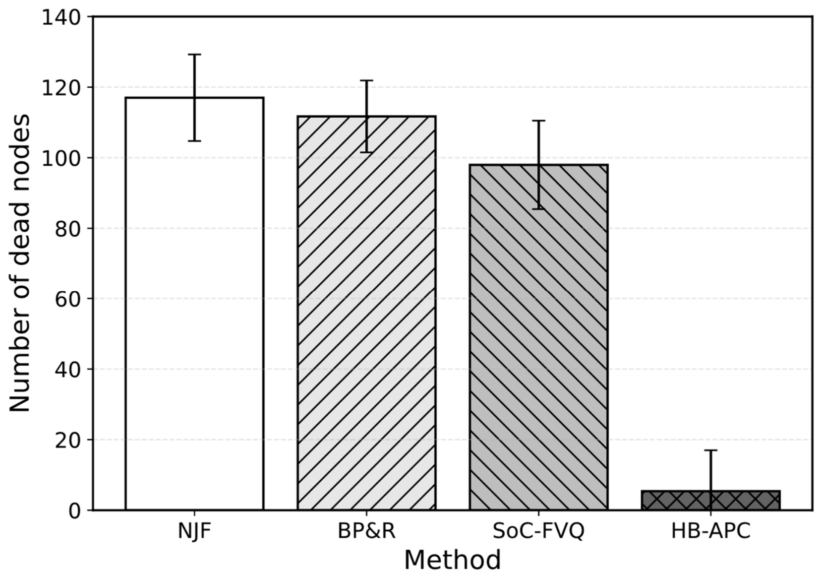
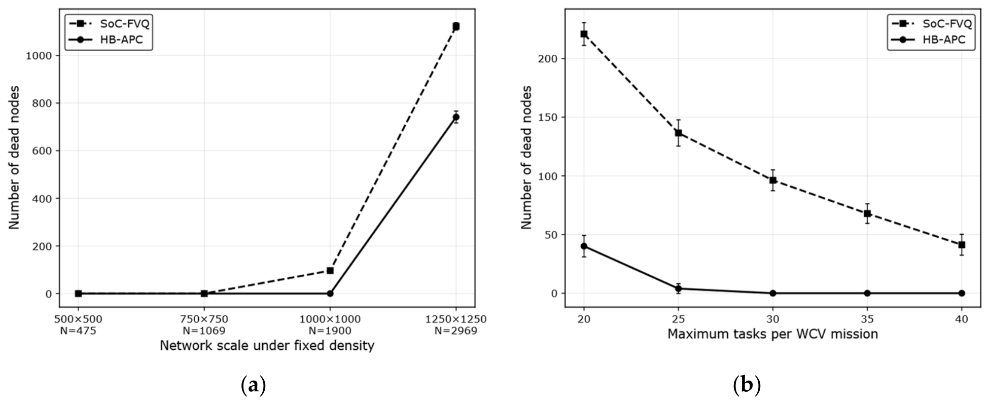
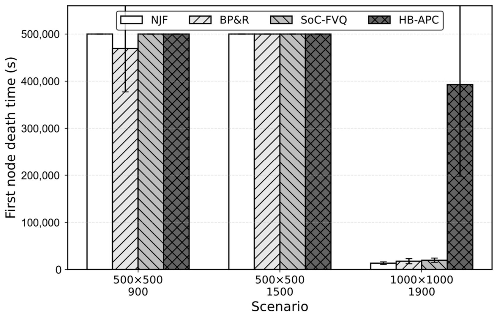
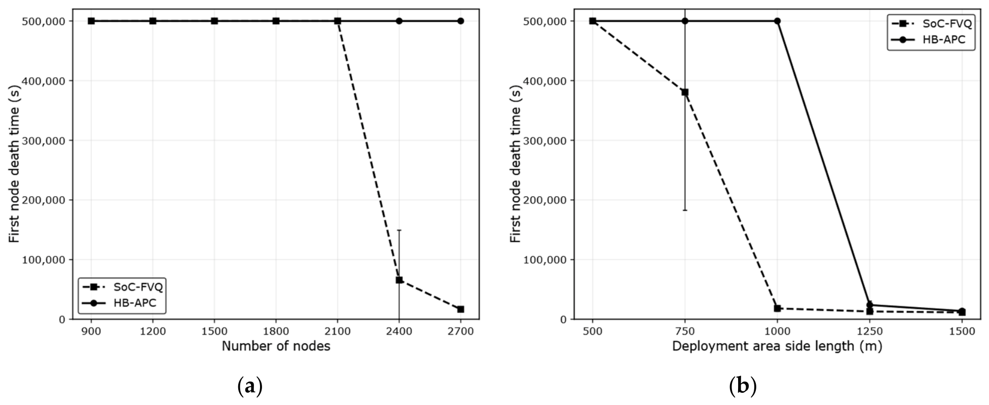
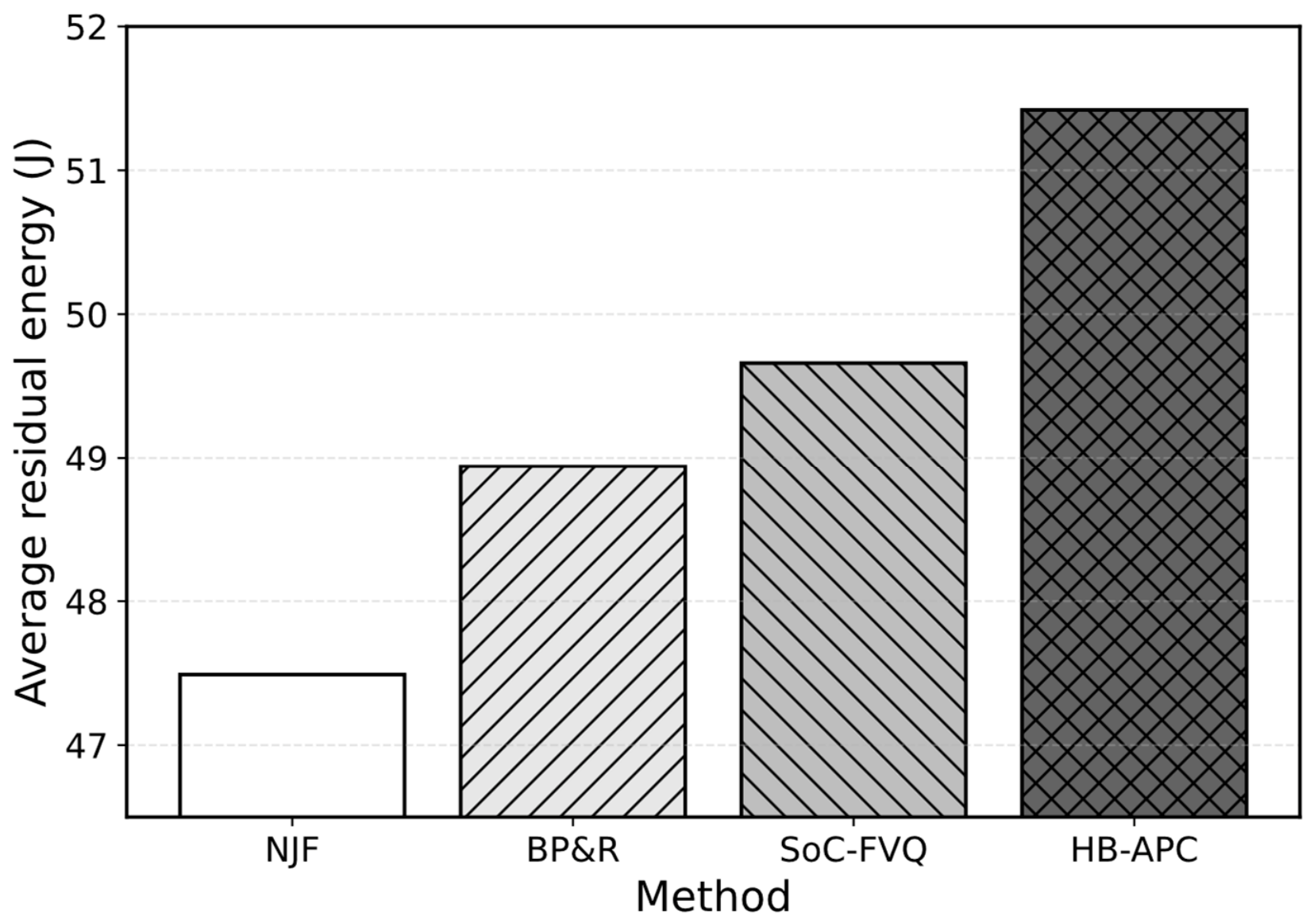
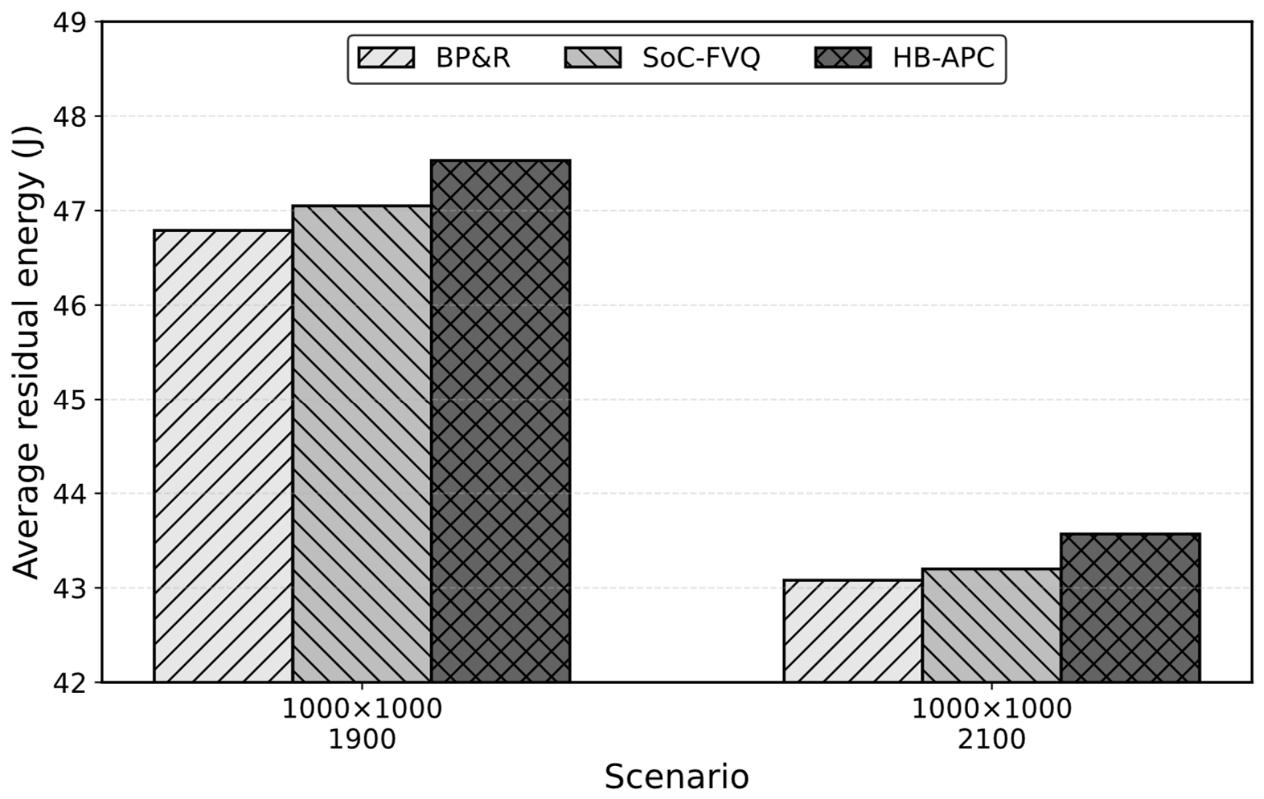
reports the overall results in static scenarios. Figure 1 focuses on node mortality in the high-pressure static scenario, Figure 2 compares FND across static scenarios, and Figure 3 shows the average residual energy in the high-pressure static scenario.

Under light and medium loads, all methods maintain stable network operation within the simulation horizon, and severe node mortality does not occur. The difference among methods becomes clear when the network enters the high-pressure regime. In the 1000 × 1000 m, 1900-node scenario, request bursts begin to dominate WCV service decisions. NJF, BP&R, and SoC-FVQ suffer from frequent request pressure or insufficient proactive protection, whereas HB-APC maintains much lower node mortality and substantially increases FND. This suggests that charging-depth control becomes most useful when survivability is limited by request congestion rather than by isolated node failures.

5.2.2. Light- and Medium-Load Scenarios

In the 500 × 500 m, 900-node scenario, NJF, SoC-FVQ, and HB-APC all achieve zero node deaths, and their FND values reach the simulation limit of 500,000 s. This indicates that the system load is not high enough to create a clear survivability gap among these methods. Nevertheless, the number of on-demand requests differs substantially. NJF generates 4578.43 requests, whereas SoC-FVQ and HB-APC generate only 156.00 and 169.63 requests, respectively. This difference shows that even when node deaths are absent, reactive on-demand scheduling may still produce a large number of explicit requests.

A similar pattern appears in the 500 × 500 m, 1500-node scenario. All methods avoid node death within the simulation horizon, but the request and travel behaviors differ. NJF produces 7614.03 on-demand requests, whereas BP&R, SoC-FVQ, and HB-APC reduce this number to 684.77, 264.13, and 383.90, respectively. HB-APC produces slightly more requests than SoC-FVQ in this scenario, but its WCV travel distance is lower than that of SoC-FVQ. This suggests that under medium load, HB-APC does not sacrifice stability, and its depth-aware decisions remain competitive in both request-pressure control and service cost.

The light- and medium-load results also clarify the operating range of HB-APC. When the WCV has enough capacity to handle current and near-future requests, the advantage of safeguarded charging is less visible in terms of node mortality. In such cases, the main benefit appears in request-pressure moderation rather than in dramatic survivability improvement.

5.2.3. High-Pressure Static Scenario

The high-pressure static scenario provides the clearest evidence of the benefit of HB-APC. In the 1000 × 1000 m, 1900-node scenario, NJF, BP&R, and SoC-FVQ result in 117.00, 111.70, and 97.97 dead nodes, respectively. HB-APC reduces this value to 5.40. This reduction is substantial and shows that the proposed method is able to prevent the large-scale node failures observed under the baselines.

The improvement is also reflected in FND. NJF, BP&R, and SoC-FVQ achieve FND values of 13,476.33 s, 17,591.13 s, and 19,705.07 s, respectively. HB-APC increases the FND to 392,720.97 s. This result indicates that HB-APC not only reduces the final number of failed nodes, but also prolongs the network lifetime.

The reason lies in the way HB-APC allocates charging depth. The safeguarded on-demand component reduces the probability that recently served nodes quickly return to the request state. Meanwhile, adaptive partial charging uses the remaining budget to delay near-future requests from proactive candidates. These two effects work together: the former stabilizes current request nodes, while the latter reduces the likelihood that new request bursts emerge immediately afterward.

Compared with SoC-FVQ, HB-APC also produces fewer on-demand requests in the high-pressure static scenario. SoC-FVQ generates 3068.40 requests, whereas HB-APC reduces this value to 1019.20. This supports the view that the gain of HB-APC is not only caused by route ordering or candidate selection. A major part of the improvement comes from charging-depth control, which changes the timing of subsequent requests.

5.2.4. Cost–Benefit Analysis in Static Scenarios

HB-APC does not always minimize WCV travel distance. In the high-pressure static scenario, HB-APC travels 1,591,719.83 m, which is higher than the 1,476,498.47 m traveled by SoC-FVQ. If travel distance were used as the only evaluation criterion, HB-APC would appear more expensive.

However, WRSN charging should be evaluated jointly from the WCV side and the network side. The additional WCV movement of HB-APC is accompanied by a much lower number of dead nodes, a longer FND, fewer on-demand requests, and higher residual energy. In the same high-pressure scenario, HB-APC achieves the highest average residual energy of 51.42 J, compared with 49.66 J for SoC-FVQ, 48.94 J for BP&R, and 47.49 J for NJF.

This result suggests that the additional WCV-side cost is not pure overhead. It is a survivability-oriented investment: the WCV spends more effort to stabilize urgent nodes and distribute partial energy to near-critical candidates. Under high-pressure conditions, minimizing travel distance alone may leave the network vulnerable to request bursts and node failures. HB-APC instead prioritizes network-side stability, which is more relevant when service capacity becomes the limiting factor.

5.2.5. Temporal Redistribution and Peak–Valley Shaping

The previous results show that HB-APC improves survivability, but survivability metrics alone do not fully explain how the improvement is achieved. To examine the underlying mechanism, this subsection analyzes the temporal distribution of charging requests.

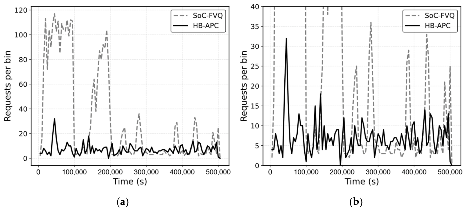
Figure 4 shows that SoC-FVQ produces clear request clusters under heterogeneous initial energy conditions, with a maximum request peak of 117 in a single time bin. In contrast, HB-APC reduces the maximum peak to 32. This result indicates that HB-APC does not merely reduce the total number of requests; it suppresses high-concurrency request bursts by redistributing request arrivals over time. Figure 4b further highlights that the request profile under HB-APC is smoother in the low-to-medium request range, which means that the WCV faces fewer instantaneous service-pressure spikes.

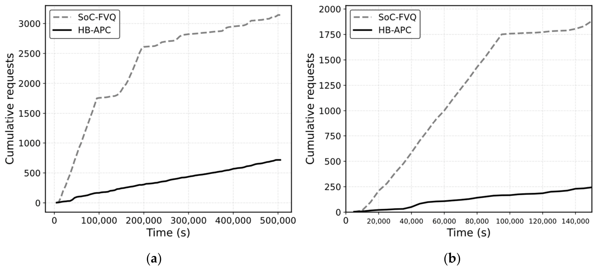
Figure 5 presents the cumulative request curves under SoC-FVQ and HB-APC. Figure 5a shows the full-scale cumulative growth over the entire simulation horizon, while Figure 5b provides a zoomed-in view of early-stage request accumulation. A steep staircase-like increase indicates that many requests arrive within a short time interval. Compared with SoC-FVQ, HB-APC exhibits a smoother cumulative growth trend, suggesting that requests are redistributed over a wider time range rather than concentrated in short bursts. This observation is consistent with the temporal-shift mechanism described in Section 4.

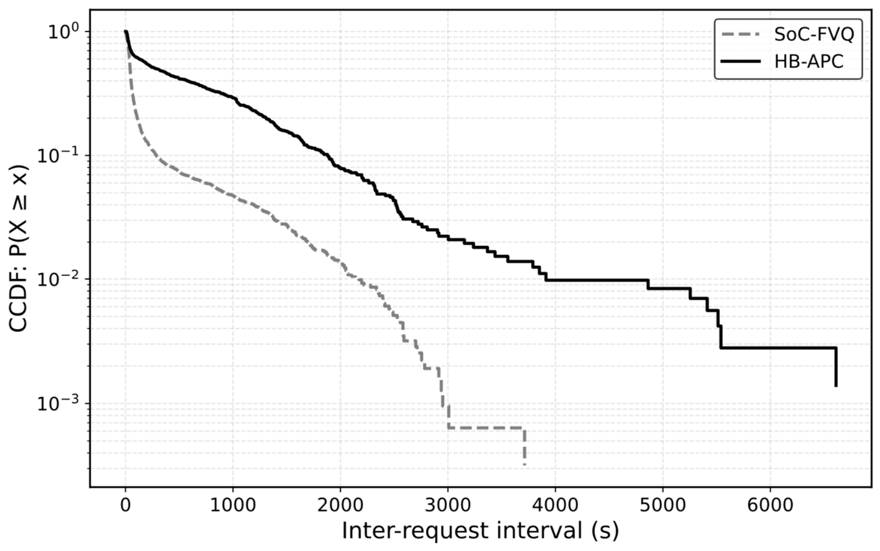
Figure 6 further analyzes inter-request intervals using the complementary cumulative distribution function (CCDF). The CCDF represents the probability that an inter-request interval is greater than or equal to a given value. Therefore, a curve that remains higher at larger interval values indicates that consecutive requests are more likely to be separated by longer time gaps.

Compared with SoC-FVQ, HB-APC maintains a higher CCDF over a wide range of inter-request intervals. This means that HB-APC produces more long inter-request gaps and reduces the frequency of rapid request succession. From the WCV’s perspective, this lowers instantaneous service pressure and provides more time to respond before nodes become depleted.

Taken together, Figure 4, Figure 5 and Figure 6 provide complementary evidence of temporal redistribution. Figure 4 shows peak suppression, Figure 5 shows smoother cumulative growth, and Figure 6 shows longer temporal separation between consecutive requests. These observations support the main claim of this paper: HB-APC does not eliminate future charging demand, but changes when that demand appears. Together with the high-pressure survivability results in Section 5.2.3, these temporal-distribution results provide evidence that HB-APC improves performance not only by selecting different nodes or changing route order, but also by reshaping future request arrivals. The reduction in request peak, smoother cumulative growth, and longer inter-request gaps reduce instantaneous WCV service pressure, which helps explain the lower number of dead nodes and longer FND observed in the high-pressure scenario.

5.3. Performance Comparison in Dynamic Scenarios

5.3.1. Purpose of Dynamic Scenario Evaluation

The static scenarios evaluate HB-APC under stable energy consumption. In practical WRSNs, however, node consumption rates may fluctuate due to event-driven sensing, communication relaying, or environmental changes. Dynamic scenarios are therefore introduced to examine whether HB-APC remains effective when energy-consumption estimates and safety-window assumptions are imperfect. In these scenarios, the actual node consumption rate is perturbed over time. As specified in Table 1, the perturbation update interval is 10,000 s, the change probability is 0.1, and the variation range is [−12.5%, +12.5%]. Thus, the dynamic scenarios represent bounded short-term workload perturbations rather than arbitrary bursty or trace-driven workload changes.

The purpose of the dynamic evaluation is not to claim that HB-APC is optimal under all perturbations. Instead, it examines whether safeguarded charging and adaptive partial charging still provide practical robustness when actual node consumption deviates from the estimated value.

5.3.2. Overall Results in Dynamic Scenarios

Before discussing the detailed trends shown in

Table 3. Overall comparison under dynamic energy-consumption scenarios. Values are reported as mean ± standard deviation over 30 independent runs. (a) Dynamic scenario results for 1000 × 1000 m, 1900 nodes; (b) Dynamic scenario results for 1000 × 1000 m, 2100 nodes.

(a)
Method	Dead Nodes	FND (s)	Requests	Distance (m)	Residual (J)
BP&R	179.53 ± 14.36	17,447.00 ± 4722.99	8675.30 ± 140.81	1,556,989.97 ± 6077.60	46.79
SoC-FVQ	176.90 ± 11.00	17,889.30 ± 3585.04	8185.47 ± 248.69	1,556,458.68 ± 4807.67	47.05
HB-APC	61.67 ± 9.38	44,240.40 ± 41,968.63	8639.37 ± 422.42	1,744,726.82 ± 17,645.75	47.53
(b)
Method	Dead Nodes	FND (s)	Requests	Distance (m)	Residual (J)
BP&R	343.80 ± 12.83	12,415.40 ± 3103.88	9346.17 ± 76.37	1,527,020.90 ± 4629.62	43.08
SoC-FVQ	343.73 ± 9.08	14,541.73 ± 2478.38	9093.20 ± 148.38	1,527,449.24 ± 4463.68	43.20
HB-APC	200.67 ± 12.04	20,176.30 ± 5275.46	9743.57 ± 110.48	1,681,455.79 ± 7706.17	43.57

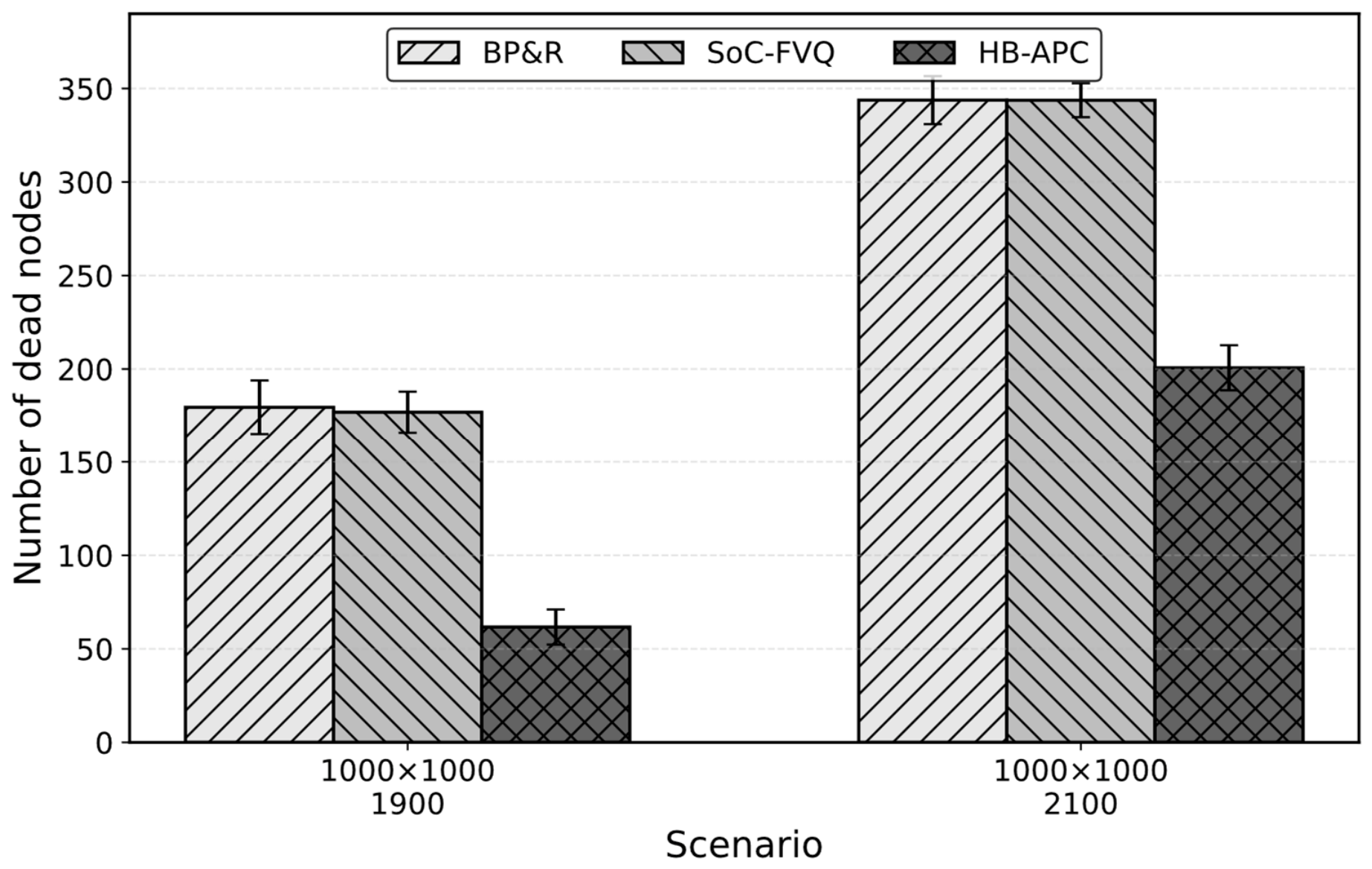
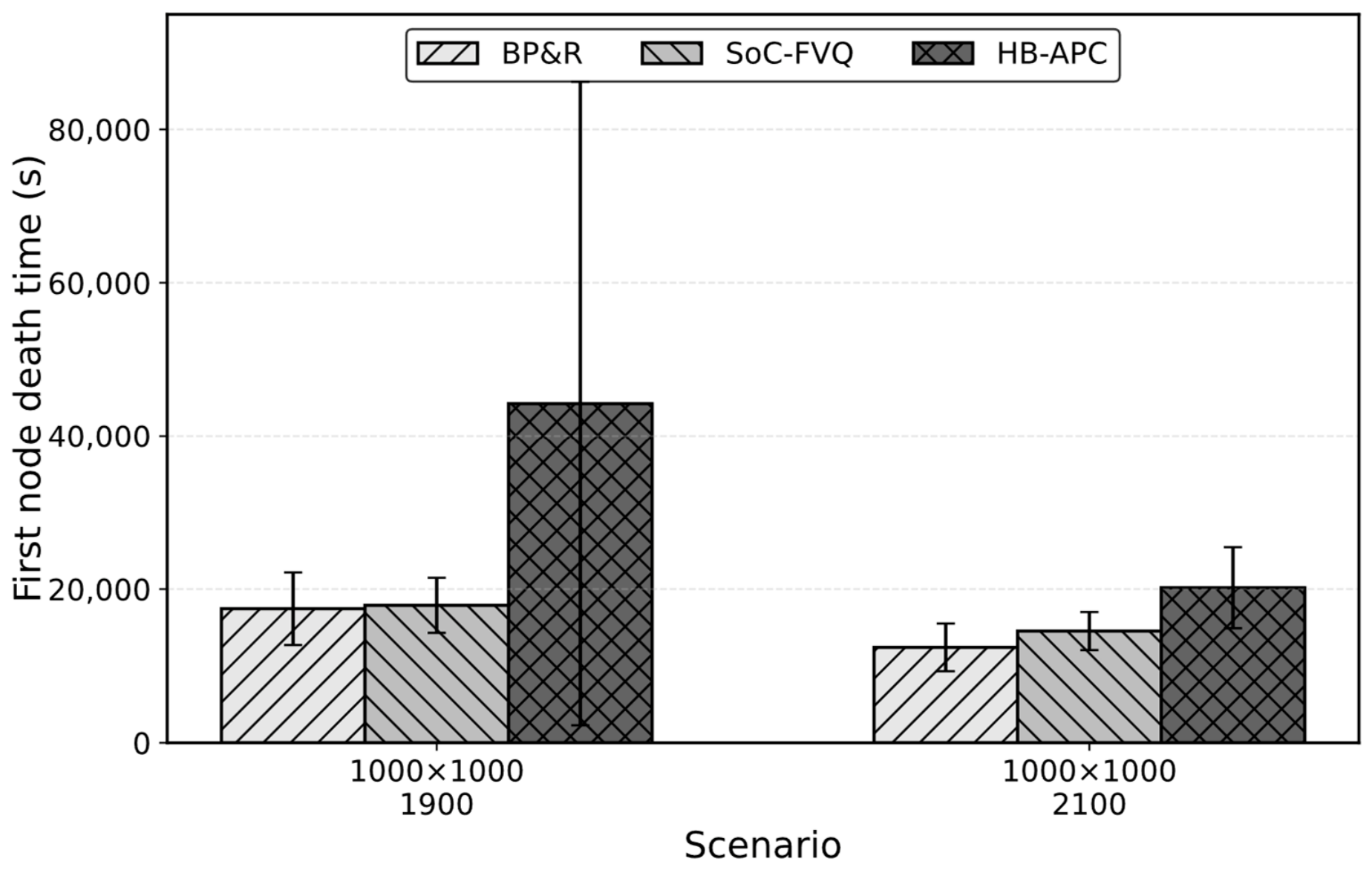
and Figure 7, Figure 8 and Figure 9, we first relate the dynamic simulation results to the short-horizon energy-consumption model in Section 3.2. The dynamic scenarios are used to examine whether the proposed charging-depth control remains effective when node consumption rates are not perfectly stable. Since the actual consumption rates vary over time, the predicted survival windows and proactive request delays may contain estimation errors. In the 1000 × 1000 m, 1900-node dynamic scenario, BP&R and SoC-FVQ produce 179.53 and 176.90 dead nodes, respectively, whereas HB-APC reduces this value to 61.67. HB-APC also achieves a FND of 44,240.40 s, compared with 17,447.00 s for BP&R and 17,889.30 s for SoC-FVQ. In the more stressful 1000 × 1000 m, 2100-node scenario, HB-APC reduces dead nodes to 200.67, compared with 343.80 for BP&R and 343.73 for SoC-FVQ, and maintains a longer FND of 20,176.30 s. These results indicate that the proposed framework remains effective under dynamic consumption-rate perturbations, even though the short-horizon energy model is an approximation.

Table 3 and Figure 7 show that HB-APC maintains a clear survivability advantage under dynamic perturbations. In the 1000 × 1000 m, 1900-node dynamic scenario, BP&R and SoC-FVQ produce 179.53 and 176.90 dead nodes, respectively. HB-APC reduces this value to 61.67. In the 2100-node scenario, the network load becomes heavier, and all methods experience more node failures. Even in this case, HB-APC reduces dead nodes to 200.67, compared with 343.80 for BP&R and 343.73 for SoC-FVQ.

Figure 8 shows a similar pattern in FND. In the 1900-node dynamic scenario, HB-APC achieves an FND of 44,240.40 s, whereas BP&R and SoC-FVQ achieve 17,447.00 s and 17,889.30 s, respectively. In the 2100-node scenario, HB-APC still maintains a longer FND of 20,176.30 s, compared with 12,415.40 s for BP&R and 14,541.73 s for SoC-FVQ.

Figure 9 further shows that HB-APC achieves the highest average residual energy in both dynamic scenarios. Although the absolute residual-energy difference is not large, it is consistent with the reductions in node mortality and the increase in FND. This consistency suggests that HB-APC improves network stability rather than only shifting failures from one metric to another.

5.3.3. Cost–Benefit Tradeoff in Dynamic Scenarios

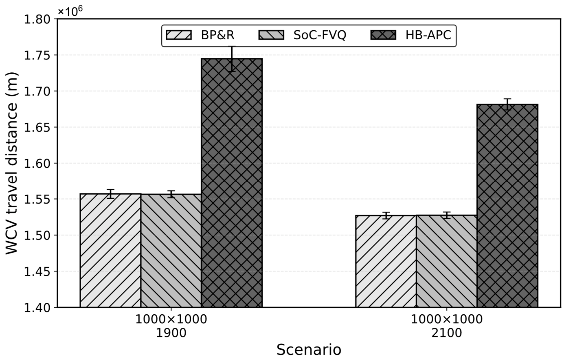
The dynamic scenarios also show that HB-APC may require higher WCV travel distance. In the 1900-node dynamic scenario, HB-APC travels 1,744,726.82 m, compared with 1,556,989.97 m for BP&R and 1,556,458.68 m for SoC-FVQ. A similar pattern appears in the 2100-node scenario, where HB-APC also travels farther than both baselines.

Figure 10 confirms that HB-APC pays additional WCV-side cost in dynamic environments. However, this cost must be interpreted together with survivability and residual-energy gains. In the 1900-node scenario, HB-APC achieves an average residual energy of 47.53 J, higher than 47.05 J for SoC-FVQ and 46.79 J for BP&R. In the 2100-node scenario, HB-APC again achieves the highest residual energy of 43.57 J, compared with 43.20 J for SoC-FVQ and 43.08 J for BP&R.

Thus, the additional travel distance reflects a tradeoff rather than an inefficiency. HB-APC spends more WCV-side effort to stabilize the network under uncertain energy consumption. Under high-pressure dynamic conditions, minimizing travel distance alone is not sufficient, because a shorter route may fail to protect enough nodes from request bursts and energy depletion.

5.3.4. Robustness Under Dynamic Energy Perturbation

The dynamic results provide evidence that HB-APC is not overly dependent on perfect energy-consumption estimation. Since the actual consumption rates change over time, the predicted survival windows and proactive request delays inevitably contain errors. If the proposed method were highly sensitive to these errors, its performance would deteriorate sharply in the dynamic scenarios. This discussion is directly related to the short-horizon energy-consumption assumption in Section 3.2, where the consumption rate is treated as an estimated mission-level value rather than a globally constant parameter. The dynamic perturbation setting specifically changes actual node consumption over time, and therefore evaluates the effect of bounded workload variation on HB-APC.

HB-APC continues to reduce node mortality and increase FND under both dynamic scenarios. In particular, the 1000 × 1000 m, 1900-node dynamic scenario shows that HB-APC reduces dead nodes to 61.67 and achieves an FND of 44,240.40 s. In the more stressful 1000 × 1000 m, 2100-node dynamic scenario, HB-APC reduces dead nodes to 200.67 and maintains an FND of 20,176.30 s. This suggests that the safeguarded charging depth provides useful tolerance against estimation errors. The guard margin prevents on-demand nodes from immediately returning to the request state when their actual consumption becomes slightly higher than expected.

The adaptive partial charging mechanism also contributes to robustness. Under higher pressure, HB-APC does not allocate excessive energy to only a small number of proactive nodes. Instead, it spreads partial energy across more candidates. This broader coverage helps reduce the risk that many nodes become critical at nearly the same time. Therefore, even under dynamic energy-consumption perturbation, HB-APC continues to moderate request concentration and improve survivability without requiring perfectly accurate long-term prediction of future request arrivals.

5.3.5. Robustness Under Prediction Errors

The preceding dynamic scenarios vary actual node energy consumption over time. To separately evaluate scheduler-side prediction errors, we keep the actual consumption rate $r_i$ unchanged and introduce noise only into the rate observed by the scheduler. For node $v_i$, the estimated consumption rate is

$${\widehat{r}}_i=r_i(1+{\epsilon }_i),{\epsilon }_i\sim U(-\eta ,\eta ),$$

where $\eta$ determines the maximum relative estimation error. The tested values are $\eta =0.00$, $0.05$, $0.10$, $0.15$, and $0.20$. The estimation error is resampled every 10,000 s to represent time-varying prediction or measurement noise. This experiment differs from the dynamic energy-consumption scenarios because it does not change the actual workload; instead, it isolates the effect of imperfect scheduler-side consumption-rate estimation. The simulation uses the 1000 × 1000 m, 1900-node scenario with $maxTask=30$, a simulation duration of 500,000 s, and staggered initial energy levels. Each setting is independently repeated 30 times.

“Runs reaching simulation limit” denotes the number of runs in which no node death occurs before the 500,000 s simulation limit. For these runs, FND is recorded as 500,000 s.

Table 4. Performance under scheduler-side prediction noise. Values are reported as mean ± standard deviation over 30 independent runs.

$\mathit{\eta }$	Method	Dead Nodes	FND (s)	Runs Reaching Simulation Limit
0.00	BP&R	$113.23\pm 11.80$	$\mathrm{17,222.27}\pm 4082.92$	0
	SoC-FVQ	$94.03\pm 10.54$	$\mathrm{21,127.80}\pm 5262.02$	0
	HB-APC	$0.00\pm 0.00$	$\mathrm{500,000.00}\pm 0.00$	30
0.05	BP&R	$111.07\pm 9.79$	$\mathrm{17,129.57}\pm 4513.36$	0
	SoC-FVQ	$99.00\pm 8.78$	$\mathrm{17,902.00}\pm 4020.23$	0
	HB-APC	$0.63\pm 1.14$	$\mathrm{364,034.77}\pm \mathrm{208,018.95}$	21
0.10	BP&R	$110.50\pm 11.53$	$\mathrm{17,485.87}\pm 4884.94$	0
	SoC-FVQ	$99.00\pm 8.78$	$\mathrm{17,902.00}\pm 4020.23$	0
	HB-APC	$0.90\pm 1.54$	$\mathrm{318,487.83}\pm \mathrm{222,637.12}$	18
0.15	BP&R	$111.53\pm 12.75$	$\mathrm{18,018.53}\pm 4972.68$	0
	SoC-FVQ	$99.00\pm 8.78$	$\mathrm{17,902.00}\pm 4020.23$	0
	HB-APC	$1.10\pm 1.80$	$\mathrm{320,468.17}\pm \mathrm{220,119.35}$	18
0.20	BP&R	$110.13\pm 11.88$	$\mathrm{16,667.13}\pm 5440.31$	0
	SoC-FVQ	$99.00\pm 8.78$	$\mathrm{17,902.00}\pm 4020.23$	0
	HB-APC	$0.97\pm 1.66$	$\mathrm{307,347.53}\pm \mathrm{220,928.05}$	17

shows that HB-APC maintains substantially better survivability across all tested prediction-noise levels, although its FND results include runs that reach the 500,000 s simulation limit. Without prediction noise, HB-APC produces no dead nodes and reaches the simulation limit in all 30 runs. At $\eta =0.20$, HB-APC produces $0.97\pm 1.66$ dead nodes and achieves an FND of $\mathrm{307,347.53}\pm \mathrm{220,928.05}$ s. In comparison, BP&R produces $110.13\pm 11.88$ dead nodes with an FND of $\mathrm{16,667.13}\pm 5440.31$ s, while SoC-FVQ produces $99.00\pm 8.78$ dead nodes with an FND of $\mathrm{17,902.00}\pm 4020.23$ s.

Across all tested noise levels, HB-APC keeps the average number of dead nodes at or below 1.10. The safeguarded charging margin reduces rapid request recurrence when actual consumption is underestimated, while pressure-aware partial charging distributes the remaining budget across multiple near-critical nodes. Consequently, HB-APC retains its survivability advantage without requiring perfectly accurate consumption-rate estimates.

Nevertheless, this simulation considers only bounded and unbiased estimation errors. Systematic bias, spatially or temporally correlated errors, delayed measurements, and abrupt prediction-model failure are not examined. Evaluating HB-APC under these more complex uncertainty patterns remains an important direction for future work.

5.4. Discussions

This subsection summarizes the simulation results according to the four evaluation questions introduced at the beginning of this section.

5.4.1. Effectiveness of Safeguarded On-Demand Charging

The static high-pressure scenario provides strong evidence that safeguarded on-demand charging is effective. HB-APC reduces dead nodes from 97.97 under SoC-FVQ to 5.40 and increases FND from 19,705.07 s to 392,720.97 s. These improvements indicate that preventing rapid re-entry into the request state is critical for network survivability.

The reduction in total on-demand requests supports the same conclusion. In the high-pressure static scenario, HB-APC produces far fewer requests than NJF, BP&R, and SoC-FVQ. This means that the safeguard mechanism does not merely delay node death; it also reduces repeated request pressure.

5.4.2. Effectiveness of Pressure-Aware Adaptive Partial Charging

The temporal request analyses in Figure 4, Figure 5 and Figure 6 show that adaptive partial charging contributes to request redistribution. Under high pressure, HB-APC does not spend the remaining budget on deep charging for only a small number of proactive nodes. Instead, it provides moderate charging to a broader set of candidates, creating multiple request-time shifts.

This behavior explains why the request peaks are lower, the cumulative request curve is smoother, and the CCDF of inter-request intervals remains higher over a wide range. These results confirm that adaptive partial charging changes the timing of future requests, not merely the amount of energy stored in individual nodes.

5.4.3. Survivability Versus Routing-Cost Reduction

The results also show that HB-APC is not designed to minimize WCV travel distance alone. In both static and dynamic high-pressure scenarios, HB-APC may travel farther than the baselines. However, this additional cost is accompanied by fewer dead nodes, longer FND, and higher residual energy.

This finding is important for WRSN evaluation. In high-pressure scenarios, a shorter route is not necessarily better if it leaves many near-critical nodes unprotected. HB-APC makes a deliberate cost–benefit tradeoff: it uses additional WCV-side effort to improve network-side survivability.

5.4.4. Network Stability Under Static and Dynamic Conditions

Across both static and dynamic scenarios, HB-APC shows the strongest advantage when the network is under high pressure. Under light and medium loads, all methods can maintain stable operation, and the difference in survivability is limited. Under high load, however, request bursts and repeated request recurrence become more damaging. In this regime, charging-depth control provides a clear benefit.

The dynamic scenarios further show that the benefit is not limited to idealized static conditions. Even when energy consumption fluctuates, HB-APC maintains lower node mortality and longer FND than the baselines. This suggests that safeguarded charging and adaptive partial charging provide practical robustness against moderate estimation errors and workload variations.

These results should not be interpreted as evidence that temporal redistribution guarantees global stability under all request-arrival patterns. Under light load, its marginal benefit is limited because the WCV already has sufficient service capacity. Under temporarily concentrated load, redistribution is effective when requests can be shifted toward lower-pressure intervals. Under persistent overload, however, it can alleviate local request peaks but cannot fully stabilize the network if the long-term charging demand exceeds the available WCV service capacity. The simulation results therefore demonstrate pressure mitigation under the evaluated operating conditions rather than a universal stability guarantee. Accordingly, temporal redistribution is not claimed to outperform existing scheduling objectives in every operating regime. Its expected advantage appears when request bursts and short-term WCV service pressure are the dominant bottlenecks. In such cases, optimizing node selection, service ordering, or travel distance alone may still fail to prevent future requests from arriving in concentrated bursts, whereas temporal redistribution directly acts on future request timing.

The static and dynamic results discussed above support the central argument of this paper: charging depth should be treated as a scheduling decision rather than a fixed service parameter. By controlling charging depth, HB-APC redistributes future request arrivals, reduces burstiness, and improves network survivability under constrained WCV mission budgets. The next subsection further examines whether these conclusions remain consistent under controlled changes in density, deployment area, network scale, and WCV service capacity.

5.5. Sensitivity Analysis of Network Scale, Density, and Service Capacity

The previous simulations compare representative operating scenarios, but they do not isolate the individual effects of node density, deployment area, network scale, and WCV service capacity. To further clarify how these factors affect FND and node mortality, we conduct controlled sensitivity simulations. In each group, one major factor is varied while the remaining settings are fixed. The comparison focuses on SoC-FVQ and HB-APC, because SoC-FVQ is the strongest semi-on-demand baseline in the high-pressure static scenario, while HB-APC represents the proposed depth-aware framework.

The first simulation examines the effect of node density under a fixed deployment area. The area is fixed at 500 × 500 m, while the number of nodes increases from 900 to 2700. As shown in Figure 11a, both methods maintain FND at the simulation limit when the number of nodes is no larger than 2100, indicating that the WCV service capacity is still sufficient in this range. When the node population reaches 2400 and 2700, SoC-FVQ begins to degrade, with FND decreasing to 65,688.77 s and 16,696.50 s, respectively. In contrast, HB-APC maintains FND at 500,000 s for all tested densities. This result shows that increasing node density raises request pressure, while HB-APC remains more robust to density-induced service pressure.

The second simulation examines the effect of deployment area under a fixed node population. The number of nodes is fixed at 1900, while the deployment area increases from 500 × 500 m to 1500 × 1500 m. In this setting, node density decreases as the area expands, while the WCV travel burden increases. Figure 11b shows that FND still decreases as the deployment area expands. SoC-FVQ drops from the simulation limit at 500 × 500 m to 18,130.33 s at 1000 × 1000 m and 11,486.63 s at 1500 × 1500 m. HB-APC remains stable up to 1000 × 1000 m, but also begins to degrade when the deployment area becomes extremely large. Nevertheless, HB-APC consistently achieves higher FND and lower node mortality than SoC-FVQ. These results indicate that deployment area affects survivability mainly through WCV travel burden and service delay, rather than through node density alone.

The third simulation fixes the node density at approximately 0.0019 nodes/m² and increases the overall network scale. The tested settings range from 500 × 500 m with 475 nodes to 1250 × 1250 m with 2969 nodes. Figure 12a shows that both methods maintain zero node deaths in the smaller-scale cases. At 1000 × 1000 m with 1900 nodes, SoC-FVQ produces 96.23 dead nodes, while HB-APC still maintains zero node deaths. At 1250 × 1250 m with 2969 nodes, both methods experience substantial degradation, but HB-APC still reduces the number of dead nodes from 1122.43 under SoC-FVQ to 741.43. This result confirms that, even under fixed density, larger network scale increases service pressure because both the travel area and the total request population increase.

The fourth simulation investigates the effect of WCV service capacity. The deployment area is fixed at 1000 × 1000 m with 1900 nodes, while the maximum number of tasks per WCV mission varies from 20 to 40. Figure 12b shows that increasing the mission capacity reduces node mortality for both methods. Under SoC-FVQ, the number of dead nodes decreases from 220.87 at maxTask = 20 to 41.27 at maxTask = 40. HB-APC decreases from 40.10 dead nodes at maxTask = 20 to 3.93 at maxTask = 25, and maintains zero node deaths when maxTask is no smaller than 30. These results indicate that HB-APC requires a lower WCV service capacity to enter a stable operating regime, because charging-depth control uses the available service budget more effectively.

Taken together, the sensitivity results show that survivability is not determined by node density alone. FND and node mortality depend on the balance between request pressure and WCV service capability, which is jointly affected by node density, deployment area, network scale, and WCV mission capacity. Across these controlled settings, HB-APC consistently improves survivability by using charging-depth control to allocate limited service capacity more effectively. These results also suggest the potential value of depth-aware temporal redistribution in larger-scale WRSNs. As the network scale increases, request bursts, local congestion, and simultaneous near-threshold nodes become more likely. A depth-aware service mechanism can help delay rapid request recurrence and distribute future request arrivals within each WCV’s service region. Therefore, the proposed concept can be combined with multi-WCV scheduling frameworks as a local charging-depth allocation module, although additional coordination is required for full multi-WCV deployment.

These sensitivity simulations also support the use of a fixed pressure-metric design. In all sensitivity settings, the weighting coefficients, pressure thresholds, and pressure-to-depth mapping are kept unchanged. Nevertheless, HB-APC maintains consistent performance advantages across different node densities, deployment areas, network scales, and WCV mission capacities. For example, when the deployment area is fixed at 500 × 500 m and the number of nodes increases from 900 to 2700, HB-APC maintains an FND of 500,000 s for all tested node populations, whereas SoC-FVQ decreases to 65,688.77 s and 16,696.50 s at 2400 and 2700 nodes, respectively. In the 1000 × 1000 m, 1900-node setting, HB-APC maintains zero dead nodes when $maxTask\ge 30$, while SoC-FVQ still produces 96.23 dead nodes at $maxTask=30$. These results indicate that the fixed pressure-metric configuration provides a stable and useful decision rule across different operating conditions without scenario-specific retuning. However, these simulations examine robustness across network conditions rather than the isolated sensitivity of each weighting coefficient, pressure threshold, or charging ratio. A systematic one-at-a-time sensitivity analysis and the derivation of theoretically optimal parameter values remain subjects for future work. Accordingly, these controlled sensitivity results provide empirical evidence of robustness rather than a formal optimality bound or approximation guarantee. They should also be interpreted within the evaluated single-WCV, single-node charging, and fixed-parameter setting. The findings support the feasibility of applying depth-aware temporal redistribution under increasing service pressure, but they do not by themselves constitute a complete multi-WCV coordination framework or establish globally optimal values for the prediction horizon, pressure thresholds, charging ratios, or safeguard coefficients. Systematic parameter optimization and multi-charger extension remain open problems.

6. Conclusions and Future Work

This work examined the role of charging depth in mobile charging for wireless rechargeable sensor networks under limited WCV mission budgets. The main argument is that charging depth should be considered together with node selection and service ordering, because it determines not only the amount of energy recovered by the current node, but also the time at which that node may issue its next charging request. This conclusion highlights the value of explicit temporal request regulation through charging-depth allocation under constrained WCV mission budgets.

Based on this observation, we proposed HB-APC, a depth-aware semi-on-demand charging framework that combines safeguarded charging for on-demand nodes with pressure-aware adaptive partial charging for proactive candidates. The safeguarded component assigns request nodes a target energy level that supports survival beyond a future service window, reducing rapid re-entry into the request state. The adaptive partial-charging component uses the remaining mission budget to delay potential future requests from near-critical nodes. Together, these two mechanisms allow the WCV to redistribute request arrivals over time rather than simply react to requests after they occur.

Simulation results show that HB-APC provides limited but stable performance differences under light and moderate loads, where severe node mortality does not occur. Its advantage becomes much more evident under high-pressure conditions. In the 1000 × 1000 m, 1900-node static scenario, HB-APC substantially reduces node mortality and achieves a longer FND than NJF, BP&R, and SoC-FVQ. The temporal request analysis further shows that HB-APC lowers request peaks, smooths cumulative request growth, and increases the separation between consecutive requests. These results support the proposed temporal redistribution mechanism.

The dynamic-scenario results also indicate that HB-APC remains effective when node energy consumption is perturbed. Although the method may introduce additional WCV-side travel or service cost, this cost is converted into network-side benefits, including fewer dead nodes, longer FND, and higher residual energy. Therefore, WRSN charging under high pressure should be evaluated not only by WCV-side cost, but also by the survivability gained from additional service effort.

Future work can extend HB-APC in several directions. First, more advanced route optimization can be integrated with the proposed depth-control mechanism to reduce unnecessary travel cost. Second, learning-based prediction models can be used to improve the estimation of node consumption rates and future request times. These prediction models should also be evaluated under trace-driven, bursty, biased, and spatially correlated workload patterns to better represent highly dynamic WRSN deployments. Third, the framework can be extended to multi-WCV or multi-node charging scenarios, where charging depth, coordination, and spatial coverage become more tightly coupled. The proposed temporal request-redistribution concept is feasible for such extensions because each WCV can still use safeguarded charging and pressure-aware adaptive partial charging as a local depth-allocation module. For large-scale multi-WCV deployment, however, this module should be integrated with charger assignment, inter-WCV route coordination, service-region partitioning, workload balancing, and cross-WCV charging-depth coordination. Formal optimization and approximation analysis can also be investigated to establish theoretical performance bounds for joint node-selection, routing, and charging-depth decisions. In addition, adaptive tuning of the safeguard window, guard margin, prediction horizon, pressure thresholds, and proactive charging ratios should be investigated to reduce reliance on fixed design settings. These extensions would further improve the applicability of depth-aware temporal redistribution in large-scale WRSNs.