Full-Night Comparison of ECG- and PPG-Derived Measures of Cardiac Variability for Sleep Disorder Screening

Abstract

Polysomnography (PSG) is the gold standard for diagnosing sleep disorders, but its complexity and cost limit widespread use. Heart rate variability (HRV) is traditionally assessed from electrocardiography (ECG), while photoplethysmography (PPG), widely available in wearable devices, offers a more accessible alternative. However, its reliability over full-night recordings remains underexplored. This study analyzes data from 50 subjects across five groups (healthy controls, rapid eye movement sleep behavior disorder, obstructive sleep apnea, periodic limb movements, and mixed comorbidities) to assess agreement between ECG-derived HRV and PPG-derived pulse rate variability (PRV), considering time-, frequency-, and nonlinear-domain features. Correlation and equivalence analyses were performed, with and without removal of artifactual segments. Correlation coefficients exceeded 0.6 for most features and improved to above 0.7 after artifact removal. Consistent improvements were observed across all subject groups. Equivalence testing further identified a subset of features showing high agreement and low bias. The results indicate that, with appropriate pre-processing, PPG can approximate ECG-derived variability in full-night sleep recordings. The identification of robust features for screening purposes supports the use of PRV for wearable-based screening and monitoring in heterogeneous sleep disorder populations.

1. Introduction

Polysomnography (PSG) is considered the gold standard for sleep assessment and the diagnosis of sleep disorders. It involves the simultaneous recording of multiple physiological signals, including electroencephalography (EEG), electromyography (EMG), electro-oculography (EOG), and electrocardiography (ECG), as well as respiratory and positional signals [1,2,3]. While PSG provides comprehensive information about sleep architecture and cardiorespiratory function, its complexity and the extensive use of sensors and electrodes can make it uncomfortable for patients and resource-intensive for clinical settings [4]. Among available signals, the ECG is commonly employed to monitor cardiac activity throughout the night, either to detect sleep-related breathing disorders, such as apneas, or to detect cardiac arrhytmias. Although less common in sleep studies, among the parameters that can be derived ECG recordings is heart rate variability (HRV), a widely recognized non-invasive marker of the autonomic nervous system regulation. In more detail, HRV represents the temporal variation between consecutive heartbeats and is commonly calculated from the R-R intervals [5].

Despite being widely regarded as the gold standard for HRV analysis, ECG presents certain limitations. First, its acquisition typically requires the use of adhesive hydrogel electrodes, which may cause discomfort during long-term monitoring or lead to skin irritation and allergic reactions in sensitive individuals [6]. Moreover, especially regarding ambulatory or sleep studies, ECG signals are often affected by noise and artifacts arising from muscle activity, electrical interference, electrode displacement, and respiration-induced baseline drift, which can significantly degrade signal quality [7,8].

To address the discomfort and practical limitations of ECG electrodes, photoplethysmography (PPG) is a widely adopted non-invasive alternative for HRV analysis [8,9,10,11,12]. It is an optical technique that detects peripheral blood volume changes and is well-suited for continuous and comfortable monitoring due to its compact size and ease of application [8,13,14].

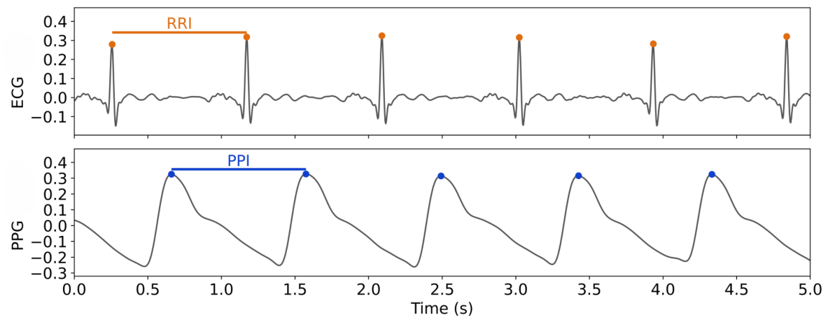
An example of ECG and PPG signals is displayed in Figure 1, with ECG R-peaks and PPG systolic peaks highlighted, together with the corresponding R-R intervals (RRI) and pulse–pulse intervals (PPI). For the sake of clarity, this paper will refer to HRV as the variability computed from ECG and pulse rate variability (PRV) as the one derived from PPG.

A strong correlation between HRV- and PRV-extracted features has been reported in the literature for healthy individuals in resting conditions [8,9,10,12,15,16,17]. However, this agreement is highly dependent on several factors, including individual characteristics, acquisition setup, underlying pathologies, and the physiological state of the subject [11]. In particular, during moderate physical or mental stress, the agreement between HRV and PRV tends to decrease, with the extent of this reduction varying across studies [18]. During intense physical activity, the correlation further deteriorates, especially for parameters describing higher frequencies of the spectrum [15]. Discrepancies have also been reported in clinical populations, such as patients with obstructive sleep apnea or cardiovascular diseases, suggesting that PRV may not reliably substitute HRV under pathological or non-ideal conditions [12,16]. Even in healthy subjects, PRV reliability is reduced in dynamic and sleep conditions due to motion artifacts, signal instability, and large inter-subject variability, limiting its interchangeability with HRV [19,20].

These discrepancies arise from both technical factors, such as motion artifacts that particularly affect PPG in ambulatory settings [18], and physiological mechanisms, including respiration-driven variations in arterial pressure, pulse transit time, and cardiac output [16]. Moreover, intrinsic differences between the electrical cardiac activity measured by ECG and the vascular and mechanical information captured by PPG further contribute to the observed divergence [16].

Additionally, most existing studies have focused on short-term recordings, typically lasting 5 to 15 min, and conducted under resting conditions or controlled experimental settings [9,10,11]. In many cases, authors selected cleaner signal segments and manually corrected peak detections [8,11,15]. Such conditions do not reflect the complexity and variability encountered during overnight sleep, where physiological states, signal quality, and autonomic regulation change substantially across sleep stages and over time.

Overall, the interchangeability between HRV and PRV remains an open research question, highlighting the need for further investigations based on long-term, real-world recordings and clinical populations to better assess the validity of PPG as a surrogate for HRV analysis.

This study aims to compare PPG-derived PRV features to ECG-derived HRV features for sleep analysis. To this end, HRV and PRV features were extracted and compared in a dataset of 50 subjects, including both healthy individuals and patients with sleep disorders, using full-night PSG recordings acquired in a real-world clinical setting. Unlike most previous studies, this approach enables a comprehensive assessment of signal quality and feature stability across the entire night, while also allowing the evaluation of how different pathological conditions may affect the agreement between the two modalities. A reliable PPG-based alternative would enable wearable monitoring solutions—such as smartwatches—capable of providing accessible and preliminary assessments of autonomic function during sleep, ultimately supporting the early detection of autonomic dysregulation.

The remainder of this paper is organized as follows. Section 2 describes the dataset and the data collection step, while Section 3 illustrates the extraction steps for HRV and PRV features, the procedures adopted for removing noisy segments, and the analyses performed to assess similarity. The results of the correlation and statistical analyses are presented in Section 4. Finally, Section 5 and Section 6 discuss the findings and provide the concluding remarks.

2. Materials

Subjects and Data

PSG recordings were collected at Molinette University Hospital in Turin (Italy), at the Regional Sleep Medicine Center. The dataset included 50 participants, divided into five groups: 10 healthy controls (HC), 10 with rapid eye movement (REM) sleep behavior disorder (RBD), 10 with obstructive sleep apnea syndrome (OSAS), 10 with periodic limb movements (PLM) and 10 with multiple comorbidities (Mixed), defined as subjects affected by two or more coexisting conditions among RBD, OSAS and PLM. Data collection complied with the Declaration of Helsinki, with approval from the Ethics Committee of A.O.U Città della Salute e della Scienza di Torino (approval number 00384/2020). Participants provided written informed consent after receiving detailed information on the study objectives and procedures. All participants had no diagnosed neurodegenerative disease and all data were properly anonymized.

Table 1. Demographic and clinical characteristics of the five subject groups included in the study. Values are reported as mean ± standard deviation. The Apnea–Hypopnea Index (AHI) represents the number of apnea and hypopnea events per hour of sleep, computed separately for REM and NREM stages.

Group	Sex (F/M)	Age (Years)	BMI (kg/m2)	AHI (REM)	AHI (NREM)
HC	3/7	35.3 ± 15.5	23.6 ± 1.4	7.9 ± 10.6	2.9 ± 2.3
RBD	5/5	50.4 ± 14.9	25.6 ± 5.3	8.3 ± 5.6	4.5 ± 4.3
OSAS	4/6	55.6 ± 12.7	28.5 ± 4.0	40.2 ± 18.5	34.4 ± 20.0
PLM	5/5	60.7 ± 17.1	25.4 ± 5.9	7.9 ± 6.1	5.2 ± 4.1
Mixed	1/9	65.5 ± 10.3	26.7 ± 4.0	37.3 ± 19.5	26.9 ± 15.4

reports the demographic and clinical characteristics of the study population, grouped by subject type.

The recordings were acquired using two portable PSG systems, namely, the Somté PSG device (Compumedics Ltd., Abbotsford, Victoria, Australia, https://www.compumedics.com.au/en/products/somte-psg/ (accessed on 1 May 2026)), and the Nox A1s^TM (Nox Medical, Reykjavík, Iceland, https://noxmedical.com/products/nox-a1-psg-system/ (accessed on 1 May 2026)).

Both devices allow for the simultaneous acquisition of multiple physiological signals, which can be exported as European Data Format files. However, for the purposes of this study, only the ECG and PPG signals were considered for the subsequent analysis. For the sake of clarity, PPG was measured from the index finger. Both the ECG and PPG were sampled at 256 Hz in the Somté device, while Nox A1s^TM sampling rates were of 200 Hz and 75 Hz for ECG and PPG, respectively. Only six subjects were recorded with the Nox A1s^TM, while the remainder were recorded using the Somté device. Given the frequency content of the signals under study (PPG: 0.5–10 Hz, ECG in PSG: 0.5–100 Hz), the sampling frequencies of both devices were more than sufficient to capture the relevant signal content and are therefore not expected to have influenced the subsequent analyses.

3. Methods

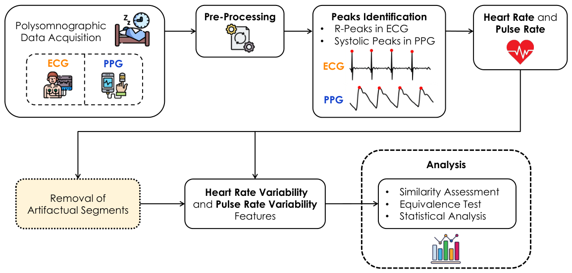
Figure 2 illustrates the overall pipeline of this work. The first step consisted of data acquisition, followed by ECG and PPG processing to obtain heart rate (HR) and pulse rate (PR). Then, these were employed for extracting HRV and PRV features; finally, a comparative analysis between those metrics was conducted. Detailed explanations of each step are provided in the following sections.

3.1. Data Analysis

Data were processed to extract relevant features for the study. All the analyses described in this section were performed using Python with custom code and toolkits (v. 3.12.3). First, sleep stages were manually scored by two experienced technicians (E.F. and S.S.), and classified as wake, N1, N2, N3 (non-REM stages, from light to deep), or REM, according to the American Academy of Sleep Medicine (AASM) guidelines [2]. The analysis was conducted only on segments scored as sleep stages, excluding segments that were either not scored or scored as wake, as these were deemed not relevant for the analysis. The mean duration of all recordings was 06:52:17 ± 01:56:10 (hh:mm:ss).

3.1.1. Signal Pre-Processing

ECG and PPG signals acquired with the Nox device were first resampled to 256 Hz to facilitate subsequent analyses by aligning sampling rates across devices. Then, to attenuate noise and motion artifacts, a fourth-order Butterworth bandpass filter (5–30 Hz, to emphasize the R-peaks) and a second-order Butterworth bandpass filter (0.5–8 Hz) [21] were applied to the raw ECG and PPG signals, respectively.

3.1.2. Peaks Identification

The Python toolbox Neurokit2 (v.0.2.12) (Documentation available at: https://neuropsychology.github.io/NeuroKit, accessed on 8 July 2025) [22] was used to identify peaks in ECG and PPG signals. In particular, an initial detection of R-peaks in the ECG and systolic peaks in the PPG was performed using the NeuroKit and Elgendi methods [21], respectively, both implemented within the library for automatic and robust peak detection.

After the initial peak identification, erroneous peaks were corrected using the kubios method [23], a correction algorithm available in the toolbox that detects, classifies, and corrects invalid peaks based on outliers in peak-to-peak interval differences.

To further reduce false detections, additional correction algorithms were specifically developed and applied to ensure that each detected peak corresponded to a local maximum. Furthermore, constraints on minimum and maximum inter-peak distances were introduced to maintain a physiologically plausible heart rate (range 35–120 bpm); an example of peak detection is provided in Figure S1 in the Supplementary Materials.

3.1.3. Feature Extraction

Based on the detected R-peaks in the ECG signal and the systolic peaks in the PPG signal, RRI and PPI were respectively computed as the temporal differences between consecutive peaks in each signal, respectively. Considering the physiological delay between ECG and PPG, the temporal trends of RRI and PPI were aligned using cross-correlation. HR and PR were then derived by converting RRI and PPI into beats per minute (bpm).

Inspection of the HR and PR signals revealed several inconsistent intervals, corresponding to noisy or irregular segments in the underlying ECG and PPG recordings that led to erroneous peak detection. These artifacts were generally limited to short time intervals. To evaluate the impact of such noise and ensure a reliable comparison between HR and PR, the corrupted segments were identified and excluded from the subsequent analysis, as described in detail in Section 3.1.4. This constitutes a first, deliberately simple and conservative approach aimed at removing only clearly corrupted segments, representing a trade-off between limiting the influence of noise and avoiding overly complex or fine-tuned procedures that might artificially affect HR–PR agreement. Accordingly, features were extracted in two separate stages: (1) from the entire signal, including noisy and artifactual segments, and (2) after removing windows affected by noise or artifacts.

In both cases, time-domain (TD), frequency-domain (FD), and nonlinear features (NLD) commonly used in HRV analysis were extracted [24], as summarized in

Table 2. Features extracted from the ECG and PPG signals, grouped according to their category: time-domain, frequency-domain, and nonlinear-domain.

Category	Feature	Description
Time Domain	MeanNN	Mean normal-to-normal (NN) intervals
	SDNN	Standard deviation of NN intervals
	RMSSD	Root mean square of successive NN intervals differences
Frequency Domain	VLF	Spectral power in the frequency band $<0.04$ Hz
	LF	Spectral power in the frequency band 0.04–0.15 Hz
	HF	Spectral power in the frequency band 0.15–0.4 Hz
	LFn	Normalized LF component
	HFn	Normalized HF component
	LF/HF	Ratio between LF and HF components
Nonlinear Domain	ApEn	Approximate Entropy: Measure of regularity and complexity of a time series
	SampEn	Sample Entropy: Measure of complexity of a physiological time series
	DFA ${\alpha }_1$	Detrended fluctuation analysis, short-term fluctuations
	DFA ${\alpha }_2$	Detrended fluctuation analysis, long-term fluctuations
	SD1	Standard deviation of Poincaré plot in direction perpendicular to the line of identity
	SD2	Standard deviation of Poincaré plot in direction parallel to the line of identity
	SD1/SD2	Ratio between SD1 and SD2

. Specifically, the full-night recordings were segmented into consecutive 5 min windows (commonly referred to as short-term) [24,25], with a 30% overlap. HRV and PRV features were computed within each window using the Neurokit2 toolbox [26]. Since $RMSSD$ is mathematically equivalent to $SD1$ (albeit on a different scale), reporting both would be redundant [27]; therefore, only $SD1$ was retained in this study, and $RMSSD$ was excluded.

3.1.4. Removal of Artifactual Segments

As introduced earlier, the detection of artifactual intervals was performed starting from the HR and PR signals, and time windows were discarded from both signals if they were considered invalid in at least one of the two.

In more detail, artifactual segments were defined as windows containing values exceeding the mean $\pm 3·$ standard deviation, and marked as outliers. A window was rejected if the number of outliers exceeded a predefined threshold ($outliers$). To avoid excluding physiologically plausible values outside this range and to make the procedure more conservative, an additional rejection criterion based on HR–PR agreement was introduced. Specifically, for windows exceeding the threshold $outliers$, the absolute difference between HR and PR was evaluated: a window was discarded if the number of samples with a discrepancy greater than $h_{\min }$ (10 or 20 bpm) was at least $samples$.

Table 3. Summary of the evaluated window rejection methods (denoted as $M1$–$M7$ in the table). Window indicates segment duration (seconds); $outliers$ is the minimum number of values exceeding the threshold required to flag a window, while $samples$ is the minimum number of points where the HR–PR difference exceeds $h_{\min }$ (bpm).

Method	Window (s)	Outliers (N)	Samples (N)	${\mathit{h}}_{\min }$ (bpm)
M1	5	1	1	20
M2	10	1	1	20
M3	20	2	2	20
M4	30	3	2	20
M5	10	1	0	20
M6	10	0	1	20
M7	10	1	1	10

summarizes the evaluated rejection methods and corresponding employed parameters. Different window lengths (5, 10, 20, and 30 s) were tested, with $outliers$ and $samples$ scaled proportionally to the window duration (see Methods 1–4). A 10 s window was ultimately selected as the optimal trade-off between signal quality and data retention, as performance differences between 5 s and 10 s were negligible, while the 10 s setting provided a more conservative choice in terms of artifact handling. In contrast, longer windows (20 s and 30 s) led to an unnecessary reduction of clean signal portions without corresponding gains in stability or robustness. For completeness, two additional approaches were also considered: rejection based solely on outliers (Method 5) and rejection based solely on HR–PR discrepancy (Method 6). Finally, Method 7 corresponds to Method 2 with a stricter threshold for $h_{\min }$ (10 bpm instead of 20 bpm).

For the remainder of this paper, All Windows denotes the case where the entire signal is retained for feature extraction (i.e., no rejection is applied), whereas Method N (e.g., $M1$–$M7$) refers to the case where artifactual segments have been removed according to the selected strategy.

3.2. Statistical Analysis and HRV-PRV Comparison

3.2.1. Similarity Assessment

The association between HRV and PRV features described in Section 3.1.3 was evaluated using both Pearson and Spearman correlation coefficients [28]. These features describe linear and monotonic associations, respectively, and provide a preliminary assessment of the relationship between the two signal modalities, given the heterogeneous nature of the computed features. Correlation coefficients (Pearson’s r and Spearman’s $\rho$) were computed per-subject for each feature, considering both the original signals (All Windows) and those obtained after the removal of noisy windows using the selected method from the proposed approach. Subsequently, for each feature, mean correlation values were calculated across all subjects. To assess inter-group variability, the average correlation values were also computed separately for each subject group (i.e., HC, RBD, OSAS, PLM, and Mixed). The distribution and variability of correlation values was examined using boxplots and quantified through the interquartile range (IQR) and the coefficient of variation (CV). To better characterize the uncertainty of the results, 95% confidence intervals (CI) were computed using subject-level bootstrap resampling. Bootstrap procedures were applied at the subject level for both All Windows and after the selected noise-removal procedure, using 5000 iterations. Finally, agreement between HRV and PRV features was further explored using Bland–Altman analysis, which also allowed the assessment of systematic bias and the limits of agreement between the two measurement methods. In addition, 95% CI were computed for the Bland-Altman analysis, following the approach described above.

3.2.2. Equivalence Testing and Statistical Analysis

Given the heterogeneity of the feature scales, to enable a consistent comparison between HRV and PRV features across subjects, all features were normalized through a cross-subject, per-feature robust scaling approach. For each feature, the median and IQR were computed by concatenating the obtained HRV and PRV values across all subjects, and used to normalize values. This procedure ensured comparability across features while reducing sensitivity to outliers.

Then, the equivalence between HRV- and PRV-derived was assessed through the Two One-Sided Tests (TOST) procedure [29], which evaluates whether the difference between two measurements lies within a predefined equivalence margin ($\epsilon$). Equivalence margins were defined relatively to the normalized feature scale; hence, $\epsilon$ values correspond to fractions of the feature variability. Specifically, values of 0.05, 0.08, 0.1, and 0.2 were selected, representing tolerances of 5, 8, 10, and 20% of the IQR, and reflecting increasing levels of acceptable deviation. Given the absence of clinically validated equivalence thresholds for HRV-PRV comparison in sleep recordings, a data-driven IQR-based definition was adopted to ensure scale-independent and comparable criteria across heterogeneous features. Moreover, these margins were selected to reflect tolerance levels appropriate for screening-oriented applications, where moderate agreement may still be acceptable in large-scale contexts.

For each feature, TOST was applied at the subject level by comparing paired HRV- and PRV-derived feature values within each participant. Hence, although features were computed from overlapping 5 min windows, they were not treated as independent observations in the equivalence analysis. Rather, equivalence was assessed separately for each subject, and established when $p<0.05$. Then, to obtain a feature-level assessment and highlight which features were more suitable for wearable-based screening, the proportion of subjects for which equivalence was demonstrated (TOST $p<0.05$) was computed for each feature. Features were then classified according to their suitability for screening, as follows:

• High Equivalence: ≥70% of subjects showing equivalence.
• Moderate Equivalence: 50–70% of subjects showing equivalence.
• Low Equivalence: ≤50% of subjects showing equivalence.

This aggregation strategy reflected the intended use in large-scale screening based on wearable devices, where stable classification across the majority of subjects is required to ensure practical applicability. To evaluate the consistency the results to the choice of $\epsilon$, the analysis was repeated for the four selected equivalence margins ($\epsilon$ = 0.05, 0.08, 0.1, 0.2). Feature robustness was defined as the proportion of $\epsilon$ values for which a feature was considered ideal or acceptable. Features consistently meeting such criteria across $\epsilon$ values were considered robust, and indicated stable equivalence across realistic tolerance levels. In addition, to improve transparency and support interpretation of mean-level differences between HRV- and PRV-derived features, 95% bootstrap CI were computed at the subject level for the mean paired differences.

Finally, to assess potential systematic differences at the subject level, distribution testing was applied to the paired HRV and PRV features. A Shapiro–Wilk test [30] was first applied to evaluate the normality of the distributions, using arrays of feature values computed every 5 min. Since most feature distributions did not meet the normality assumption, the non-parametric Wilcoxon signed-rank test [31] was selected for pairwise sample comparison; a significance level of $\alpha =0.05$ was adopted. In addition to p-values, effect sizes were computed to quantify the magnitude of the observed differences beyond statistical significance. In this study, Wilcoxon tests and effect sizes were used for complementary purposes and to characterize systematic bias between HRV and PRV to support interpretation of the results, rather than as unique criteria for feature selection. In particular, features showing statistically significant differences ($p<0.05$) were not excluded if equivalence was previously demonstrated through the TOST procedure. Effect sizes were instead used to provide additional context on the magnitude of bias and to support the interpretation and comparative ranking of features in terms of robustness.

The described statistical analyses were conducted for the two selected pre-processing pipelines (All Windows and the selected rejection method), and feature equivalence and robustness were evaluated independently for each method. Comparative analyses focused on the consistency of equivalence across all $\epsilon$ values, with particular emphasis on features that remained robust throughout the application of the selected rejection method, to assess its suitability for PRV-based screening applications.

4. Results

4.1. Selection of the Window Rejection Method

Table 4. Percentage of signal removed for each tested window rejection method (mean ± standard deviation, minimum and maximum values).

Method	Mean ± STD (%)	Min (%)	Max (%)
M1	2.04 ± 1.51	0.41	7.45
M2	3.54 ± 2.44	0.79	9.75
M3	6.23 ± 4.18	1.37	19.42
M4	8.89 ± 5.87	2.12	28.31
M5	7.98 ± 6.44	1.86	35.05
M6	4.02 ± 2.72	0.86	11.09
M7	4.41 ± 2.87	1.04	12.33

reports the percentage of signal removed (mean ± standard deviation, with minimum and maximum values across subjects) for each tested method.

The optimal method was selected by jointly considering the amount of discarded signal and the resulting correlations between HRV- and PRV-derived features were considered (reported in Tables S2 and S3 in the Supplementary Materials).

Among the evaluated configurations, $M3$ and $M4$ yielded only marginal improvements in correlation, whereas the remaining methods led to more substantial increases. In particular, $M1$ showed low correlation while also removing the smallest fraction of segments, likely because the 5 s window is too short to reliably capture artifactual behavior. Conversely, $M5$ produced the highest percentage of removed windows, as it relies solely on the number of outliers; indeed, in some cases this can lead to the exclusion of segments that still exhibit good agreement between HR and PR. $M6$ and $M7$ achieved some of the highest correlation values; however, they were found to be overly selective. Specifically, $M6$ relies exclusively on the HR–PR differences, while $M7$ applies a particularly strict threshold on allowable bpm discrepancies.

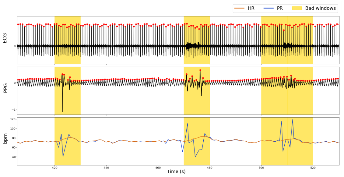
Based on these considerations, M2 was selected as the optimal trade-off, balancing improved correlation, moderate signal removal, and robustness in identifying noisy segments without being overly restrictive (Figure 3). As shown in Figure S2 in the Supplementary Materials, following the application of M2, the temporal trends of the features exhibit greater overlap, indicating improved agreement between HRV- and PRV-derived metrics.

Table 5. Percentage of signal removed with the selected method M2. The mean ± standard deviation, minimum and maximum are reported for each category (HC, RBD, OSAS, PLM, Mixed).

Group	Mean ± STD (%)	Min (%)	Max (%)
HC	2.80 ± 1.69	0.88	5.90
RBD	4.00 ± 2.89	0.79	9.75
OSAS	3.52 ± 2.71	1.23	9.43
PLM	3.20 ± 1.70	0.83	6.45
Mixed	4.20 ± 2.66	1.70	9.16

reports the proportion of segments identified as noisy and removed using M2, across subject groups. As appreciable, the rejected percentage remains below 10% for all subjects (8.14 ± 1.81%), with the lowest values observed in the HC group.

4.2. Correlation Between Heart- and Pulse-Derived Features

As described in Section 3.2.1, correlation analyses were performed between HRV and PRV features under both the All Windows condition and after removal of noisy segments. Tables S2 and S3 in the Supplementary Materials report the average Pearson and Spearman correlation coefficients between HRV and PRV features for the different methods, computed across all subjects. Supplementary Table S4 reports the median correlation values for both methods alongside the 95% CI, and Supplementary Figure S4 displays the CI range.

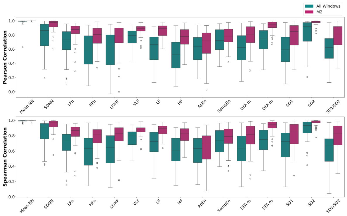
Overall, correlation values increased after applying M2 in all extracted features, indicating improved association between HRV and PRV after exclusion of low-quality windows. A comprehensive comparison of correlation values between All Windows and M2 is shown in Supplementary Figure S3. Under the All Windows condition, Pearson’s r values were consistently above 0.5, with 66.7% of features exceeding 0.6. After applying M2, correlations further improved, with all features exceeding 0.7, except for $ApEn$, which remained slightly lower (0.66). A similar trend was observed for Spearman’s $\rho$, with most features exceeding 0.7 after M2, while $ApEn$ again showed a lower value (0.64).

In addition to increasing correlation values, M2 also reduced variability across subjects. As shown in Figure 4, the distribution of both Pearson and Spearman coefficients becomes narrower after removal of artifactual segments, with a noticeable reduction in dispersion. This is reflected in lower IQR and higher median values compared to All Windows, indicating more consistent agreement between subjects. This reduction in variability is further supported by the analysis of additional metrics, with both the CV and IQR decreasing after applying M2 (Figures S5 and S6 in the Supplementary Materials).

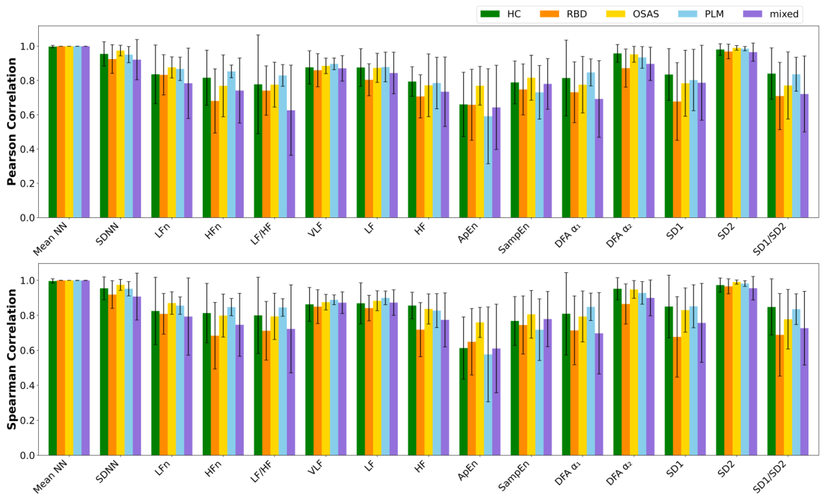
Figure 5 presents the correlation values by subject group. Higher agreement is generally observed in HC, OSAS, and PLM subjects, whereas lower values are found in the RBD and Mixed group. Despite this inter-group differences, the application of M2 consistently improved correlation across all groups, although some variability within subjects persists. However, sub-group analyses are reported in an exploratory and descriptive framework due to the limited sample size within each clinical group.

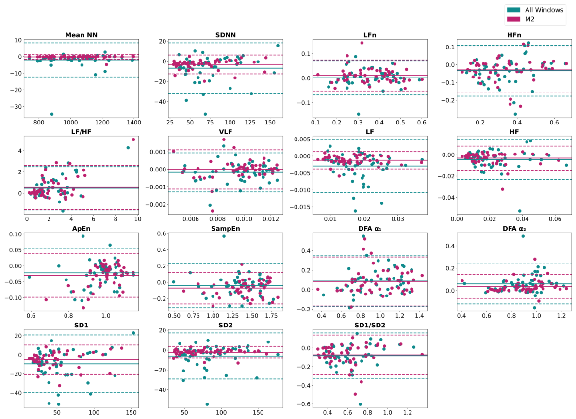
Finally, agreement between HRV and PRV was further evaluated using Bland-Altman analysis (Figure 6); Supplementary Table S5 further reports the Bland–Altman bias for each feature together with its 95% bootstrap CI, for both the All Windows and M2 conditions, providing an estimate of the uncertainty of the systematic difference between HRV and PRV. Following the application of M2, limits of agreement decreased for most features, indicating reduced dispersion between the two measures. In addition, the mean difference between HRV and PRV approached zero for the majority of features, suggesting a considerable reduction in systematic bias. However, a residual bias remains for specific features (as appreciable for $LFn$, $LF/HF$, $ApEn$, $SampEn$, and $SD1/SD2$) which continue to show a non-negligible difference even after noise removal.

4.3. Equivalence and Bias Analysis

Since correlation and Bland–Altman analyses describe the strength of association and the presence of systematic bias between HRV and PRV features, formal evaluation of whether the observed differences are acceptable for practical use in clinical screening studies was conducted. This approach is grounded on the idea that high correlation does not imply agreement, and small but statistically significant biases may still be compatible with screening applications, provided that accurate correction is performed. To address this, as described in Section 3.2.2, a TOST procedure was applied, complemented with a Wilcoxon signed-rank test to further characterize residual bias.

Table 6. Percentage of subjects for which each HRV feature is equivalent to the corresponding PRV feature, evaluated across different equivalence margins ($\epsilon$). For each epsilon, results are reported for the original full signal (All Windows, AW) and after removing noisy windows (M2). 🟉: indicates features that showed an increase in equivalence after cleaning.

Feature	$\mathit{\epsilon }=0.05$		$\mathit{\epsilon }=0.08$		$\mathit{\epsilon }=0.1$		$\mathit{\epsilon }=0.2$
	AW	M2	AW	M2	AW	M2	AW	M2
MeanNN	98%	100% 🟉	98%	100% 🟉	98%	100% 🟉	100%	100%
SDNN	14%	38% 🟉	26%	58% 🟉	34%	72% 🟉	66%	88% 🟉
LFn	4%	10% 🟉	22%	34% 🟉	32%	44% 🟉	74%	80% 🟉
HFn	10%	18% 🟉	26%	34% 🟉	30%	40% 🟉	52%	72% 🟉
LF/HF	10%	14% 🟉	14%	22% 🟉	18%	28% 🟉	42%	48% 🟉
VLF	10%	28% 🟉	40%	66% 🟉	56%	84% 🟉	90%	92% 🟉
LF	2%	16% 🟉	10%	28% 🟉	18%	34% 🟉	52%	82% 🟉
HF	2%	10% 🟉	8%	18% 🟉	16%	36% 🟉	36%	58% 🟉
ApEn	4%	4%	14%	16% 🟉	22%	26% 🟉	50%	52% 🟉
SampEn	10%	2%	18%	16%	28%	24%	52%	54% 🟉
DFA ${\alpha }_1$	10%	32% 🟉	18%	46% 🟉	22%	36% 🟉	44%	56% 🟉
DFA ${\alpha }_2$	6%	46% 🟉	16%	24% 🟉	24%	54% 🟉	52%	72% 🟉
SD1	6%	16% 🟉	10%	24% 🟉	20%	28% 🟉	34%	62% 🟉
SD2	16%	66% 🟉	42%	82% 🟉	52%	88% 🟉	76%	96% 🟉
SD1/SD2	6%	12% 🟉	10%	20% 🟉	20%	22% 🟉	36%	46% 🟉

reports the equivalence summary for All Windows and M2, across all tested equivalence margins ($\epsilon$), and reports the robustness of features to the choice of $\epsilon$. Specifically, for each feature, the proportion of subjects satisfying the equivalence criterion was computed, providing a measure of both agreement and robustness. Overall, the application of M2 resulted in a substantial increase in the percentage of subjects satisfying equivalence compared to the All Windows condition.

In more detail, for $\epsilon$ = 0.2, 8 out of 15 features demonstrated high equivalence (i.e., ≥70% of subjects), while 5 showed moderate, and 2 low (average: 47%). Similar trends were observed across the other equivalence margins, with more stringent $\epsilon$ values leading to a reduction in the number of features meeting the equivalence criterion, as expected.

As appreciable, some features ($MeanNN$, $SDNN$, $VLF$, $SD2$) demonstrated good agreement across multiple $\epsilon$ values, indicating stable equivalence between HRV and PRV representations. Specifically, $MeanNN$ exhibited 100% concordance in all tested $\epsilon$ values with M2, and thus it could be considered reliable even with strict equivalence margins. Moderate-to-high equivalence was found for $SDNN$, $VLF$, and $SD2$ at values of $\epsilon$ = [0.08, 0.1], suggesting their reliability in real-world scenarios, where inter-subject variability is high. Conversely, other features ($HFn$, $LFn$, $LF/HF$, $LF$, $DFA{\alpha }_1$, $DFA{\alpha }_2$, $SD1$) exhibited sensitivity to the choice of $\epsilon$, suggesting that their agreement depends on the tolerated level of deviation, and thus might not be adequate for use in screening purposes.

To complement the equivalence analysis, as described earlier, the Wilcoxon signed-rank test was used to assess the extent of systematic differences between HRV and PRV features, previously investigated with Bland–Altman plots (cf. Section 4.2). The percentage of subjects for which no significant difference was observed ($p>$ 0.05) was computed for each feature, along with the average effect size together with its 95% bootstrap CI. Subject-level CI for mean differences are reported in detail in Supplementary Table S6.

The results show that for some of the other extracted features, statistically significant differences persist across subjects, despite high equivalence rates observed with TOST, revealing moderate-to-high percentage of bias.

In particular, for $\epsilon$ = 0.2, features $SDNN$, $LFn$, $HFn$, $LF$, $HF$, $DFA{\alpha }_2$, $SD1$ and $SD2$ exhibited moderate-to-high equivalence rate, but relatively low percentage of non-significant Wilcoxon results, indicating the presence of consistent bias, though small, as previously highlighted through the Bland–Altman analysis. A similar trend is observed for $\epsilon$ = 0.1 (with $SDNN$, $SD2$, $DFA{\alpha }_2$) and $\epsilon$ = 0.08 ($SDNN$, $SD2$). Effect size analysis revealed small-to-moderate effect sizes, suggesting that these differences remain limited in magnitude.

On the other hand, $MeanNN$, describing the average time between successive heartbeats, consistently exhibited very low percentage of bias across all tested $\epsilon$ margins. Similarly, $VLF$ (which exhibited moderate-to-high equivalence rate for $\epsilon$ = [0.08, 0.1, 0.2]) consistently showed low bias in the tested subjects.

Overall, these results suggest that a large subset of features achieves practical equivalence between HRV and PRV, particularly after the application of M2. Residual biases identified through the Wilcoxon test are generally small and do not preclude the use of these features in screening contexts, where approximate agreement is considered sufficient.

4.4. Practical Implications for Screening

Based on the integrated assessment of TOST equivalence, Wilcoxon characterization, and effect size analysis, practical recommendations for feature use in screening applications were formulated. Features were hence classified according to a two-tier framework: (1) a primary classification based on TOST equivalence rate (i.e., percentage of subjects meeting the equivalence criterion, as described in the previous section), and (2) a complementary evaluation integrating Wilcoxon test results and effect size to characterize bias properties and variability.

Features achieving equivalence above 70% were deemed suitable for screening and were further stratified according to the presence and magnitude of bias. Specifically, features exhibiting both high equivalence and no significant bias were assigned a “High Suitability” label. Features with high equivalence but systematic bias and small effect sizes (below 0.5) were classified as “Suitability with bias correction”, as the observed bias, although statistically significant, remained within acceptable equivalence margins and could potentially be corrected with linear transformation. Features with moderate equivalence (50–70%) and favorable Wilcoxon characteristics (e.g., low bias percentage, small effect size) were assigned a “Conditional Suitability” recommendation, and considered appropriate for screening only when combined with more robust features. Conversely, features achieving moderate TOST equivalence (50–70%) but exhibiting unfavorable bias characteristics, or features with high variability (large effect sizes irrespective of equivalence rate), were classified as “Supplementary Features”, appropriate exclusively as auxiliary indicators rather than primary screening metrics. Finally, features failing to meet the 50% equivalence threshold were classified as “Not Recommended” for screening applications.

Table 7. Results of the integrated, two-level analysis. For each tested equivalence margin ($\epsilon$), the Table reports the best features, along with the percentage of equivalence assessed through TOST, the percentage of subjects for which no bias was observed through Wilcoxon test (WI), the effect size [Lower CI, Upper CI], and the practical recommendation for use in screening scenarios.

Feature	TOST	WI	Effect Size	Recommendation
$\epsilon =0.05$
MeanNN	100%	70%	0.157 [0.129, 0.189]	High Suitability
SD2	66%	6%	0.605 [0.537, 0.668]	Supplementary Feature
$\epsilon =0.08$
MeanNN	100%	70%	0.157 [0.129, 0.189]	High Suitability
SDNN	58%	8%	0.631 [0.568, 0.692]	Supplementary Feature
VLF	66%	66%	0.162 [0.125, 0.200]	Supplementary Feature
SD2	82%	6%	0.605 [0.537, 0.668]	Conditional Suitability
$\epsilon =0.1$
MeanNN	100%	70%	0.157 [0.129, 0.189]	High Suitability
SDNN	72%	8%	0.631 [0.568, 0.692]	Conditional Suitability
VLF	84%	66%	0.162 [0.125, 0.200]	Suitability (Bias Correction)
DFA ${\alpha }_2$	54%	16%	0.526 [0.451, 0.600]	Supplementary Feature
SD2	88%	6%	0.605 [0.537, 0.668]	Conditional Suitability
$\epsilon =0.2$
MeanNN	100%	70%	0.157 [0.129, 0.189]	High Suitability
SDNN	88%	8%	0.632 [0.568, 0.692]	Conditional Suitability
VLF	92%	66%	0.162 [0.125, 0.200]	Suitability (Bias Correction)
LF	82%	18%	0.347 [0.298, 0.397]	Suitability (Bias Correction)
SD2	96%	6%	0.605 [0.537, 0.668]	Conditional Suitability

reports the recommendations for the best features in each of the explored equivalence margins; features that remain equivalent across multiple $\epsilon$ thresholds indicate higher robustness and suitability for large-scale screening applications.

As mentioned in the previous Section, $MeanNN$ consistently exhibited high equivalence and low bias across all explored $\epsilon$ values, and was assigned a “High Suitability” label in all configurations.

This pragmatic classification prioritizes equivalence as the primary criterion while acknowledging that small, consistent biases do not preclude clinical utility in preliminary screening contexts, where subsequent confirmatory testing with gold standard PSG is performed.

5. Discussion

This study aimed to compare HRV derived from ECG and PRV derived from PPG in full-night PSG recordings, including both healthy individuals and patients with sleep disorders. In particular, the role of signal pre-processing was investigated to determine whether the removal of artifactual segments could improve the reliability of PRV as a surrogate for HRV in long-term monitoring and clinically heterogeneous conditions.

Overall, the results demonstrate good concordance between HRV and PRV features, supporting the use of PPG as a possible alternative to ECG for estimating cardiac variability in full-night sleep recordings. These findings are in line with previous studies reporting good correspondence between HRV and PRV in healthy subjects [8,18,32].

However, earlier work has mainly focused on short-term recordings or controlled experimental settings, typically limited to 5–15 min [9,10,11], and did not include clinical populations. In contrast, the present study extends this comparison to full-night recordings across multiple subject groups. Despite the increased complexity associated with prolonged monitoring and the presence of pathological conditions, correlations between ECG- and PPG-derived features remained generally high, with most features exceeding 0.7. Importantly, the removal of artifactual segments using the selected pre-processing method (M2) consistently improved correlation across all features. This emphasizes the importance of artifact handling in long-term recordings, where signal quality may fluctuate. Residual variability in correlation values is still observed, reflecting both inter-subject differences and intra-group heterogeneity. These variations may be associated with differences in disease severity as well as individual physiological characteristics. This observation aligns with previous studies indicating that PRV can be influenced by signal quality, motion artifacts, and underlying pathophysiological conditions [12,16].

Moreover, the analysis of the extracted features identified a subset showing consistent equivalence across the explored margins, suggesting higher robustness and suitability for large-scale screening applications. In particular, MeanNN exhibited high equivalence and low bias across all $\epsilon$ margins, indicating reliability in clinical contexts. $VLF$ showed high equivalence for $\epsilon$ = [0.1, 0.2], despite a residual systematic bias. However, the relatively small effect size (0.162) suggested that this feature may still be usable for screening purposes after appropriate bias correction. Conversely, features such as $SD2$ and $SDNN$ showed only moderate equivalence through TOST, together with substantial bias and moderate-to-large effect sizes (0.605 and 0.631, respectively). In these cases, bias correction alone is unlikely to be sufficient, and these features should either considered as support-only (e.g., $SD2$ at $\epsilon$ = 0.05 and $SDNN$ at $\epsilon$ = 0.08), or used with caution under less stringent equivalence margins.

Despite these encouraging results, some limitations should be acknowledged. First, group-wise analyses revealed variability both across subjects and within each clinical group. Although participants were categorized by disease type, individual differences in disease severity and subject-specific factors persist within each group and may influence the results. However, given that the objective of this study is to assess the suitability of PPG for screening applications rather than fine-grained diagnostics, the observed variability does not undermine the overall robustness of this approach.

Second, the extracted features exhibited heterogeneous behavior across domains. In particular, time-domain features (e.g., $MeanNN$, $SDNN$) generally showed greater stability between ECG and PPG, whereas some frequency-domain features were less consistent, particularly normalized indices and ratios (e.g., $LF/HF$). Nonlinear features appeared to be the most challenging, with measures such as $ApEn$ showing lower robustness compared to alternative features such as $SampEn$ or $DFA$ exponents. These differences, together with the considerations on the usability of features, highlight the importance of careful feature selection, depending on the intended application. From a physiological perspective, such domain-dependent behavior may be influenced by multiple interacting factors, including pulse transit time, peripheral vascular dynamics, and modality-specific acquisition characteristics. However, disentangling these effects was beyond the scope of the present study, which primarily focused on the technical comparison between ECG- and PPG-derived metrics. Future studies involving dedicated physiological and clinical analyses will be required to better interpret these mechanisms and their impact on wearable-derived biomarkers.

Third, the proposed method for detecting and removing artifactual relied on the simultaneous availability of ECG and PPG signals. While this requirement was necessary in the present study to enable a controlled comparison between modalities, it inhrently limits direct applicability in real-world scenarios based on wearable or consumer-grade technologies. Furthermore, the proposed cleaning strategy was intentionally designed to be simple and conservative, targeting only clearly corrupted segments rather than performing fine-grained artifact removal. This choice aimed to balance improvements in signal quality and minimal intervention on the original recordings. Nevertheless, future work will focus on developing more advanced and fully modality-independent noise detection strategies, with particular emphasis on PPG-only approaches, to enhance applicability in real-world wearable and consumer-grade settings.

Another aspect to consider is the heterogeneity of the acquisition systems used in this study. Although the sampling frequencies of both ECG and PPG were adequate for capturing the physiological signals of interest and all recordings were processed using a consistent pipeline, differences in sensor technology and acquisition conditions may still introduce variability that was not explicitly quantified in the present work. Future studies will investigate the robustness of the proposed approach across ambulatory and wearable platforms to further support its generalizability.

Finally, although the study includes multiple subject groups, the overall cohort size remains relatively small (50 subjects in total, with only 10 subjects per clinical group), which may limit generalizability to broader and more heterogeneous clinical populations. Importantly, sub-group analyses should be interpreted as exploratory and descriptive in nature, given the limited sample size per group; these results should therefore be regarded as preliminary and require validation in larger and more diverse cohorts. Future studies will include larger populations spanning different demographic and clinical characteristics to confirm the robustness of the observed findings.

6. Conclusions

This study demonstrates that PPG-derived PRV features approximate ECG-derived HRV features over full-night PSG recordings, even in heterogeneous populations including healthy subjects and patients with various sleep disorders. Careful pre-processing, particularly regarding the removal of artifactual segments, substantially demonstrated improved agreement between HRV and PRV features, thus mitigating variability due to motion artifacts or signal quality. Most features showed strong correlations (above 0.7), with time-domain features and certain nonlinear measures being the most stable, while some frequency-domain and nonlinear features, such as $ApEn$, were more sensitive to noise.

These findings extend previous evidence from short-term, controlled studies [9,10,11] to longer recordings and clinical populations, supporting the validity of PPG as a reliable surrogate for HRV assessment under real-world conditions. The results also emphasize the importance of careful feature selection and pre-processing to ensure consistent PRV estimation, particularly for frequency-domain and nonlinear features.

Overall, this work supports the development of wearable-based screening systems relying primarily on PPG and other wrist-derived signals to detect deviations from physiological sleep. While such systems are not intended to replace PSG, they offer a scalable and less invasive solution for large-scale pre-screening. In clinical practice, this approach could facilitate the early identification of individuals requiring comprehensive overnight evaluation, thereby reducing the burden on sleep laboratories and optimizing the allocation of diagnostic resources.

Looking ahead, the validation of such observations in larger and more diverse cohorts and the definition of robust and reproducible automated artifact detection methods (possibly based solely on PPG) could further enhance the robustness and applicability of PRV for both long-term monitoring and screening of sleep disorders.

Further studies are required to evaluate the feasibility and robustness of this approach in truly wearable-based settings, where signal acquisition is less controlled and subject to higher levels of motion artifacts and environmental noise. Furthermore, recent advances in high-sensitivity measurement of pulsatile blood flow, specifically Speckleplethysmography (SpG) [33] and Diffuse Speckle Pulsatile Flowmetry (DSPF) [34], offer promising opportunities to enhance traditional PPG-based cardiovascular monitoring and should be further explored in future studies.

References

1. Medical Advisory Secretariat. Polysomnography in patients with obstructive sleep apnea: An evidence-based analysis. Ont. Health Technol. Assess. Ser. 2006, 6, 1–38. [Google Scholar] [PubMed]
2. American Academy of Sleep Medicine. The AASM Manual for the Scoring of Sleep and Associated Events: Rules, Terminology and Technical Specifications; Version 2.4; American Academy of Sleep Medicine: Darien, IL, USA, 2017. [Google Scholar]
3. Chesson, A.L., Jr.; Ferber, R.A.; Fry, J.M.; Grigg-Damberger, M.; Hartse, K.M.; Hurwitz, T.D.; Johnson, S.; Kader, G.A.; Littner, M.; Rosen, G.; et al. The indications for polysomnography and related procedures. Sleep 1997, 20, 423–487. [Google Scholar] [CrossRef] [PubMed]
4. Tabar, Y.R.; Mikkelsen, K.B.; Rank, M.L.; Farahani, F.; Olsen, M.; de Zambotti, M.; Baker, F.C.; Møller, A.M.; Dinesen, P.T.; Arendt-Nielsen, L. Ear-EEG for sleep assessment: A comparison with actigraphy and PSG. Sleep Breath. 2021, 25, 1693–1705. [Google Scholar] [CrossRef] [PubMed]
5. Karim, N.; Hasan, J.; Ali, S.S. Heart rate variability—A review. J. Basic Appl. Sci. 2011, 7, 71–77. [Google Scholar]
6. Patel, V.; Danish, M.; Monteleone, C. All Roads “Lead” to Anaphylaxis: Hypersensitivity to Electrocardiogram Leads. Ann. Allergy Asthma Immunol. 2018, 121, S82. [Google Scholar] [CrossRef]
7. Rudiger, A.; Hellermann, J.P.; Mukherjee, R.; Follath, F.; Turina, J. Electrocardiographic artifacts due to electrode misplacement and their frequency in different clinical settings. Am. J. Emerg. Med. 2007, 25, 174–177. [Google Scholar] [CrossRef] [PubMed]
8. Lu, G.; Yang, F.; Taylor, J.; Stein, J. A comparison of photoplethysmography and ECG recording to analyse heart rate variability in healthy subjects. J. Med. Eng. Technol. 2009, 33, 634–641. [Google Scholar] [CrossRef] [PubMed]
9. Selvaraj, N.; Jaryal, A.; Santhosh, J.; Deepak, K.K.; Anand, S. Assessment of heart rate variability derived from finger-tip photoplethysmography as compared to electrocardiography. J. Med. Eng. Technol. 2008, 32, 479–484. [Google Scholar] [CrossRef] [PubMed]
10. Mirescu, Ş.C.; Harden, S.W. Photoplethysmography as a Potential Alternative to Electrocardiography for Recording Heart Rate Intervals Used in Variability Analysis. J. Med. Life 2012, 5, 123–128. [Google Scholar] [PubMed]
11. Jeyhani, V.; Mahdiani, S.; Peltokangas, M.; Vehkaoja, A. Comparison of HRV parameters derived from photoplethysmography and electrocardiography signals. In Proceedings of the 2015 37th Annual International Conference of the IEEE Engineering in Medicine and Biology Society (EMBC); IEEE: Piscataway, NJ, USA, 2015; pp. 5952–5955. [Google Scholar] [CrossRef] [PubMed]
12. Pinheiro, N.; Couceiro, R.; Henriques, J.; Muehlsteff, J.; Quintal, I.; Goncalves, L.; Carvalho, P. Can PPG be used for HRV analysis? In Proceedings of the 2016 38th Annual International Conference of the IEEE Engineering in Medicine and Biology Society (EMBC); IEEE: Piscataway, NJ, USA, 2016; pp. 2945–2949. [Google Scholar] [CrossRef] [PubMed]
13. Challoner, A.; Ramsay, C. A photoelectric plethysmograph for the measurement of cutaneous blood flow. Phys. Med. Biol. 1974, 19, 317–328. [Google Scholar] [CrossRef] [PubMed]
14. Jago, J.R.; Murray, A. Repeatability of peripheral pulse measurements on ears, fingers and toes using photoelectric plethysmography. Clin. Phys. Physiol. Meas. 1988, 9, 319. [Google Scholar] [CrossRef] [PubMed]
15. Lin, W.H.; Wu, D.; Li, C.; Zhang, H.; Zhang, Y. Comparison of Heart Rate Variability from PPG with That from ECG. In The International Conference on Health Informatics; Zhang, Y., Ed.; IFMBE Proceedings; Springer: Cham, Switzerland, 2014; Volume 42, pp. 213–217. [Google Scholar] [CrossRef]
16. Khandoker, A.H.; Karmakar, C.K.; Palaniswami, M. Comparison of pulse rate variability with heart rate variability during obstructive sleep apnea. Med. Eng. Phys. 2011, 33, 204–209. [Google Scholar] [CrossRef] [PubMed]
17. Lu, S.; Zhao, H.; Ju, K.; Shin, K.H.; Lee, M.; Shelley, K.; Chon, K.H. Can photoplethysmography variability serve as an alternative approach to obtain heart rate variability information? J. Clin. Monit. Comput. 2008, 22, 23–29. [Google Scholar] [CrossRef] [PubMed]
18. Schäfer, A.; Vagedes, J. How accurate is pulse rate variability as an estimate of heart rate variability? A review on studies comparing photoplethysmographic technology with an electrocardiogram. Int. J. Cardiol. 2013, 166, 15–29. [Google Scholar] [CrossRef] [PubMed]
19. Chang, F.; Chang, C.; Chiu, C.; Hsu, S.; Lin, Y. Variations of HRV analysis in different approaches. In Proceedings of the 2007 Computers in Cardiology; IEEE: Piscataway, NJ, USA, 2007; pp. 17–20. [Google Scholar] [CrossRef]
20. Lu, G.; Yang, F. Limitations of Oximetry to Measure Heart Rate Variability Measures. Cardiovasc. Eng. 2009, 9, 119–125. [Google Scholar] [CrossRef] [PubMed]
21. Elgendi, M.; Norton, I.; Brearley, M.; Abbott, D.; Schuurmans, D. Systolic Peak Detection in Acceleration Photoplethysmograms Measured from Emergency Responders in Tropical Conditions. PLoS ONE 2013, 8, e76585. [Google Scholar] [CrossRef] [PubMed]
22. Makowski, D.; Pham, T.; Lau, J.Z.; Chang, A.; Desormeaux, M.; Chartier, S.; Moreau, D. NeuroKit2: A Python toolbox for neurophysiological signal processing. Behav. Res. Methods 2021, 53, 1689–1696. [Google Scholar] [CrossRef] [PubMed]
23. Lipponen, J.; Tarvainen, M. A robust algorithm for heart rate variability time series artefact correction using novel beat classification. J. Med. Eng. Technol. 2019, 43, 173–181. [Google Scholar] [CrossRef] [PubMed]
24. Shaffer, F.; Ginsberg, J.P. An Overview of Heart Rate Variability Metrics and Norms. Front. Public Health 2017, 5, 258. [Google Scholar] [CrossRef] [PubMed]
25. Sandercock, G.R.H.; Bromley, P.D.; Brodie, D.A. The reliability of short-term measurements of heart rate variability. Int. J. Cardiol. 2005, 103, 238–247. [Google Scholar] [CrossRef] [PubMed]
26. Pham, T.; Lau, Z.J.; Chen, S.H.A.; Makowski, D. Heart Rate Variability in Psychology: A Review of HRV Indices and an Analysis Tutorial. Sensors 2021, 21, 3998. [Google Scholar] [CrossRef] [PubMed]
27. Ciccone, A.B.; Siedlik, J.A.; Wecht, J.M.; Deckert, J.A.; Nguyen, N.D.; Weir, J.P. Reminder: RMSSD and SD1 are identical heart rate variability metrics. Muscle Nerve 2017, 56, 674–678. [Google Scholar] [CrossRef] [PubMed]
28. Schober, P.; Boer, C.; Schwarte, L.A. Correlation Coefficients: Appropriate Use and Interpretation. Anesth. Analg. 2018, 126, 1763–1768. [Google Scholar] [CrossRef] [PubMed]
29. Lakens, D. Equivalence tests: A practical primer for t tests, correlations, and meta-analyses. Soc. Psychol. Personal. Sci. 2017, 8, 355–362. [Google Scholar] [CrossRef] [PubMed]
30. Shapiro, S.S.; Wilk, M.B. An Analysis of Variance Test for Normality (Complete Samples). Biometrika 1965, 52, 591–611. [Google Scholar] [CrossRef]
31. Woolson, R.F. Wilcoxon signed-rank test. In Wiley Encyclopedia of Clinical Trials; Wiley: Hoboken, NJ, USA, 2007; pp. 1–3. [Google Scholar]
32. Gil, E.; Orini, M.; Bailón, R.; Vergara, J.; Mainardi, L.; Laguna, P. Photoplethysmography pulse rate variability as a surrogate measurement of heart rate variability during non-stationary conditions. Physiol. Meas. 2010, 31, 1271–1290. [Google Scholar] [CrossRef] [PubMed]
33. Dunn, C.E.; Monroe, D.C.; Crouzet, C.; Hicks, J.W.; Choi, B. Speckleplethysmographic (SPG) Estimation of Heart Rate Variability During an Orthostatic Challenge. Sci. Rep. 2019, 9, 14079. [Google Scholar] [CrossRef] [PubMed]
34. Bi, R.; Du, Y.; Singh, G.; Ho, J.H.; Zhang, S.; Attia, A.B.E.; Li, X.; Olivo, M.C. Fast pulsatile blood flow measurement in deep tissue through a multimode detection fiber. J. Biomed. Opt. 2020, 25, 055003. [Google Scholar] [CrossRef] [PubMed]
Figure 1. Simultaneous visualization of ECG and PPG signals. Orange dots on the ECG trace indicate R peaks, from which the RRI is computed. Blue dots on the PPG trace mark the systolic peaks, used to calculate the PPI.
Algorithms 19 00531 g001
Figure 2. Visual summary of the analysis pipeline. ECG and PPG signals were collected and pre-processed, followed by extraction of HRV and PRV features. Finally, a comparative analysis was performed to assess the similarity between HRV and PRV.
Algorithms 19 00531 g002
Figure 3. Excerpt of ECG and PPG signals with detected peaks (red dots), along with HR (solid orange line) and PR (solid blue line). Artifactual segments identified with M2 are highlighted in yellow.
Algorithms 19 00531 g003
Figure 4. Boxplots of Pearson (top) and Spearman (bottom) correlations for all features, comparing All Windows signal (in teal) with the cleaned signal after M2 rejection (in magenta).
Algorithms 19 00531 g004
Figure 5. Average Pearson (top) and Spearman correlations (bottom), grouped by subject category: HC (green), RBD (orange), OSAS (yellow), PLM (blue) and Mixed (purple). Correlations were calculated on the features after removing noisy windows (M2).
Algorithms 19 00531 g005
Figure 6. Bland–Altman plots for each variable comparing HRV and PRV features. Each point represents the mean value of the feature for a single subject. The x-axis shows the average of HRV and PRV values, while the y-axis shows their difference. Solid line: mean difference; dotted lines: 95% limits of agreement.
Algorithms 19 00531 g006