Article

Imputation Bias in ARIMA Air Quality Models

Department of Computer Science, University of East London, London E16 2RD, UK
*
Authors to whom correspondence should be addressed.
Algorithms 2026, 19(6), 449; https://doi.org/10.3390/a19060449
Submission received: 15 March 2026 / Revised: 21 May 2026 / Accepted: 25 May 2026 / Published: 2 June 2026
(This article belongs to the Special Issue Advances in Deep Learning-Based Data Analysis)

Abstract

Missing data remains a pervasive challenge in air quality data analysis, where inappropriate imputation techniques can introduce hidden biases and compromise the reliability of time-series models such as AutoRegressive Integrated Moving Average (ARIMA). This paper examines the impact of linear interpolation and mean/median imputation on the performance of the ARIMA model and biases in the prediction of fine particulate matter 2.5 (PM2.5) concentration, together with a detailed analysis of ARIMA generated error metrics and their implications for the accuracy and reliability of the prediction. The findings reveal that package-default imputation significantly influences ARIMA forecasts, while mean/median imputation consistently delivers superior predictive performance, highlighting its robustness for handling missing environmental data. Moreover, imputation during the data transformation stage exerts a greater influence on model outcomes than methods applied at later analysis stages.

1. Introduction

Predicting air quality in urban environments has become a critical aspect of modern urban planning and public health initiatives, as evidenced by the increasing concerns surrounding air pollution in major cities around the world [1,2]. Accurate forecasting of pollutants such as fine particulate matter 2.5 (PM2.5) is crucial for effective environmental governance and public health protection. Pollutants within the atmosphere are complex and require sophisticated sensor-based monitoring stations. Despite their fundamental role in data acquisition, these stations frequently face issues such as missing data, which can significantly impair the reliability of predictive models [3]. The challenge itself stems from the intricate interplay of environmental factors and the inherent limitations of sensor technology, which can lead to gaps in crucial time-series datasets [2]. Similarly, data professionals use their own judgement in choosing appropriate imputation techniques, which can introduce hidden biases in time-series-based auto-regressive integrated moving average (ARIMA) models used for air quality prediction [4].
Bias is one of the significant challenges in time series data analysis, particularly when dealing with incomplete environmental datasets, as the selection of an imputation method can subtly influence the underlying data distribution and subsequent model outcomes [5,6]. When it comes to time-series forecasting, ARIMA is one of the most widely recognised and applied statistical models, offering robust capabilities to capture temporal dependencies and trends in air quality data [7,8]. However, the efficacy of ARIMA models is inherently linked to the completeness and quality of the input data, making the choice of imputation technique a critical factor in mitigating hidden biases that could skew air quality predictions [4]. This article investigates how different imputation strategies for handling missing environmental data can introduce subtle, yet significant, biases into ARIMA models, thereby affecting the accuracy and reliability of air quality predictions. This research focuses on quantifying these biases and proposing methodologies to mitigate their impact, ultimately improving the robustness of air quality forecasting. The general hypothesis of this study is that the selection of imputation methods for missing time-series data in air quality monitoring profoundly affects the bias and precision of subsequent ARIMA models, thereby necessitating a systematic comparison of these methods to ensure reliable forecasting [9].
Finally, this article offers practical recommendations for data scientists and researchers to improve the precision and reliability of air quality predictions when dealing with incomplete datasets. This comprehensive analysis bridges the gap between theoretical imputation techniques and their practical implications, ensuring that air quality models are not only statistically sound but also ecologically relevant. This practical understanding and guidance not only minimise the risk of bias, but also enhances social value through informed decision-making for environmental policies and public health interventions required by central and local government bodies.

2. Related Work

The climate data landscape has seen significant transformation in recent years, as the scientific community has recognised the critical role that data play in understanding and addressing the challenges posed by climate change. For example, air pollution data have become indispensable for researchers and policy makers seeking to measure and mitigate the environmental consequences of human actions [10,11]. Another example is the use of cutting-edge advanced technologies such as remote sensing and internet of things (IoT) devices to gather unprecedented amounts of data on environmental conditions [10]. IoT devices can provide real-time information on factors such as temperature, humidity, and air quality, enabling more dynamic and responsive environmental monitoring [12,13]. IoT devices have played a pivotal role in enhancing local-scale climate monitoring efforts by local authorities in London, United Kingdom (UK). The London metropolitan area consists of 33 local authorities, each with unique environmental characteristics and required to meet specific regulations such as the Department of Environment, Food & Rural Affair’s (DEFRA) Air Quality Management guidelines [14,15]. London authorities use climate data for real-time pollution detection, identifying hotspots, and informing urban planning decisions to mitigate environmental risks [16]. This granular data collection also facilitates more precise and proactive climate action strategies, for example, close monitoring of air quality to assess the effectiveness of low-emission zones or to launch public health campaigns where pollution levels are critically high. Although IoT sensors in air quality monitoring stations are well calibrated to UK and EU standards, challenges remain to ensure data interoperability across diverse monitoring networks and address the significant costs associated with sensor maintenance and calibration [17].
Globally, climate data projected via IoT devices have now become widely available, providing researchers with a wealth of information to rigorously examine the climate systems of the Earth. At the same time, the abundance of air quality data has presented new challenges, including the most common issue of missing values, which can significantly hinder robust analysis and predictive modelling [4,18]. Data professionals often wrestle with the decision between deleting incomplete records or employing imputation techniques to fill the gaps, a decision that profoundly influences the integrity and representativeness of the dataset [19]. Indeed, the inability to analyse and handle missing data can substantially impede the air quality data analysis process. For example, incorrect imputation can lead to skewed distributions, altered temporal dependencies, and, ultimately, biased air quality predictions [4,18]. Furthermore, biased air quality modelling can propagate errors in policy decisions, undermining efforts to mitigate environmental risks and protect public health [11,20]. The existing literature extensively explores various imputation methods, ranging from simple statistical approaches to complex machine learning algorithms, each with its own assumptions and suitability depending on the nature of the missing-ness and the characteristics of the time series [21]. However, a comprehensive understanding of how these choices specifically introduce and propagate bias within the autoregressive integrated moving average framework for air quality prediction remains less thoroughly investigated.
The field of air quality prediction has seen extensive research, with various models ranging from statistical approaches to advanced machine learning and deep learning techniques being applied [1]. ARIMA forecasting models are foundational for time-series analysis, offering robust capabilities to capture temporal dependencies and trends in air quality data [2]. However, the efficacy of ARIMA models is inherently linked to the completeness and quality of the input data, making the choice of imputation technique a critical factor in mitigating hidden biases that could skew air quality predictions [22]. ARIMA statistical methods can be implemented through various open source packages. Although these packages facilitate forecasting models, their performance is critically dependent on the quality and completeness of the time series data, some of the packages include functions to tackle missing values, for example, the ‘forecast’ package in R provides functionalities for handling gaps, although its effectiveness is limited for longer periods of contiguous missing-ness [23].
In addition to statistical methods such as autoregressive integrated moving average (ARIMA), deep learning and machine learning approaches have gained prominence for their ability to model complex non-linear relationships and interactions within air quality datasets [24]. For example, hybrid deep learning models that integrate Kalman filtering with bi-directional gated recurrent units, optimised via Chi-square divergence, have shown promise in air quality index forecasting by effectively handling data distribution uncertainty [25]. Similarly, advanced machine learning techniques such as random forests and gradient boost excel at modelling non-linear relationships and integrating diverse predictors to provide dynamic gap-filling strategies for PM2.5 time series data [26]. Despite these advances, ARIMA models remain fundamental for time-series forecasting due to their interpretability and established theoretical foundation, often serving as a baseline against which more complex models are evaluated [27]. Moreover, ARIMA models explicitly capture seasonality, trends, and autoregressive components within a single framework, making them particularly suitable for environmental time series that exhibit such regular patterns [28].
Air quality data often contains significant gaps due to sensor malfunctions or maintenance, which can reach up to 5% of the total dataset, thus requiring sophisticated gap-filling techniques to maintain the integrity of the time-series analysis [24]. In such scenarios, where the missing-ness is substantial, the limitations of simpler imputation methods become apparent, as they often fail to capture the complex pollution dynamics or accurately represent peak pollution hours over multi-day gaps [26]. The existing literature highlights various imputation techniques, from classic mean to median interpolation and more advanced statistical methods, such as linear regression imputation, each possessing distinct advantages and disadvantages depending on the nature and extent of missing data [29]. Advanced data science encompasses numerous imputation techniques, ranging from sophisticated statistical models and machine learning-based approaches to hybrid methods that integrate multiple strategies to improve accuracy and robustness [30,31]. Despite its importance, data imputation remains one of the least studied but most critical steps in preparing air quality datasets, directly influencing the reliability and validity of subsequent analyses and predictive modelling [32]. Air quality data that includes time series measurements of various pollutants, meteorological conditions, and sensor calibration data pose a multifaceted challenge to impute missing values [4]. The existing literature broadly addresses challenges in handling missing data in time series, particularly when gaps are extensive or occur non-randomly [4]. However, identifying the most effective imputation strategies for multivariate air quality time series, especially their impact on the subsequent performance of the ARIMA model, remains an under-explored area that requires further investigation [20].
The article explores the most common imputation methods and evaluates their impact on the performance of ARIMA models for the prediction of air quality. Specifically, this study investigates how different imputation techniques, when applied to environmental datasets with high missing information rates, can inadvertently introduce systematic bias into forecasts generated by ARIMA models, ultimately compromising the reliability of air quality assessments.
To provide greater clarity and ensure common understanding, this paper identifies the research gaps and contributions as follows, presented in bullet points:

2.1. Research Gaps

  • Limited understanding of how commonly used imputation methods influence bias in ARIMA-based air quality forecasting.
  • Inadequate evaluation of how preprocessing decisions propagate errors into time-series prediction models.
  • Lack of focused studies isolating the effect of missing-data treatment from other modelling factors.

2.2. Contribution of This Study

  • Systematic comparison of linear interpolation and mean/median imputation methods.
  • Quantitative analysis of how the imputation choices affect the accuracy of the ARIMA forecast and the error metrics.
  • Demonstration that preprocessing-stage imputation significantly impacts model bias and reliability.
  • Provision of practical insights for handling missing data in environmental time-series analysis.

2.3. Study Limitations

  • This study used a controlled univariate forecasting framework, using a single monitoring dataset and selected baseline imputation methods. Although this setup facilitates the clear isolation and evaluation of imputation-induced biases in ARIMA modelling, it does not fully capture the complexity of real world air quality forecasting systems in which meteorological variables, emission dynamics, spatial variability, and advanced multivariate models can substantially influence predictions. Consequently, the findings should be interpreted as relevant to comparative imputation analysis rather than as a universal forecasting solution.
  • The dataset used in this research comprises hourly PM2.5 concentration measurements from a single monitoring station, thus limited for spatial variations in air pollution levels.
  • The analysis of PM2.5 concentrations does not incorporate meteorological variables, such as temperature, humidity, and wind speed, which are known to influence pollutant dispersion and concentration levels.
  • The study focuses exclusively on mean/median imputation and linear interpolation, overlooking other known imputation techniques.

3. Materials and Methods

3.1. Air Quality Dataset

This article specifically addresses bias challenges by evaluating the performance of ARIMA models under various imputation strategies, aiming to identify methods that minimise bias and enhance prediction accuracy. The dataset comprises an hourly air quality measurement of PM2.5 concentrations collected over a five-year period from 1 January 2019 to 31 December 2023, from a monitoring station located in Wren Close, London, United Kingdom. This particular dataset is ideal for examining the effects of various imputation techniques on time-series forecasting due to its inherent seasonal and daily patterns, as well as the presence of varied missing data. The selected monitoring site is managed by Air Quality England on behalf of the London Borough of Newham, and the data was accessed and extracted from their publicly available open-source data platform [33].
The hourly PM2.5 concentration data was measured using a regulatory-grade instrument known as BAM (beta attenuation monitor), which operates on the principle of beta ray attenuation to determine mass concentrations of particulate matter [34]. This method offers high precision and reliability, making the collected data a solid foundation for evaluating imputation strategies and their impact on forecasting models [24]. Air Quality England (AQE) is a well known resource for environmental data in the United Kingdom, often employed in air quality research due to its comprehensive and systematically curated datasets. All datasets provided are aligned with the local air quality management (LAQM) framework, which confirms its consistency and quality standards that meet the DEFRA technical guidance of the UK [14].

3.2. Proposed Methodology

The details of the methodological framework employed in this study involved various steps and they are as follows.
  • Data Exploration and Transformation.
  • Implementation of the baseline ARIMA Model.
  • Implementation of Package’s Imputation Technique.
  • Implementation of the Mean/Median Imputation Technique.

3.2.1. Data Exploration and Transformation

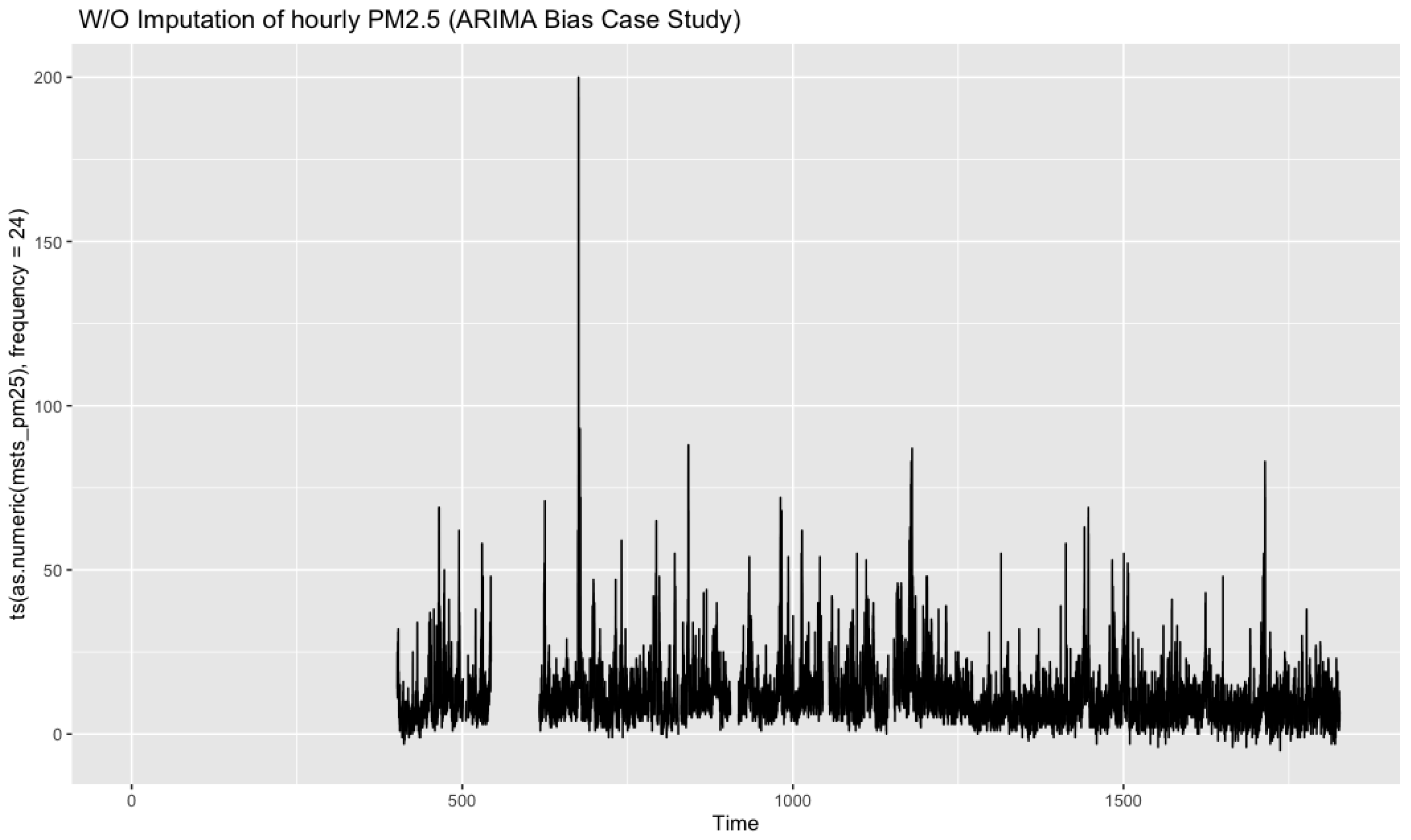
Initially, raw hourly PM2.5 concentration data was extracted, followed by a thorough exploratory data analysis to identify preliminary trends, seasonality, and the extent of missing values. Preliminary data analysis revealed that PM2.5 has in total 43,824 hourly observations, of which 12,664 were missing, representing approximately 28.9% of the total dataset, a significantly high rate that requires robust imputation strategies for subsequent modelling. Figure 1 below illustrates the distribution of missing values in the dataset, highlighting periods of consecutive missing observations and their potential impact on the continuity of the time series. Data missing in time series, particularly within the environmental data analysis lifecycle, arise from various factors, such as sensor failures, data transmission errors, misapplied calibration measurements, or power outages at monitoring stations [1,35]. Addressing missing gaps is quite critical, as untreated missing data can compromise the statistical validity of time-series models such as ARIMA and lead to biased parameter estimates, ultimately affecting the reliability of air quality predictions [4].
After exploratory data analysis, the dataset was subjected to several preprocessing transformations, including the elimination of extraneous pollutant variables and the detection and removal of outliers by statistical techniques. These procedures were implemented to maintain the integrity of the data and prepare the data for subsequent time-series analysis and the application of various imputation methods.

3.2.2. Implementation of Baseline ARIMA Model

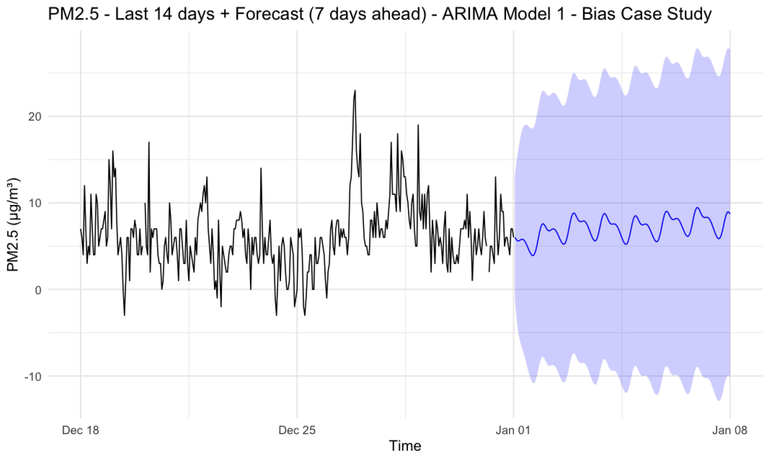
A baseline ARIMA model was established using pre-processed PM2.5 data to serve as a comparative benchmark for evaluating the impact of different imputation strategies on model performance. This foundational model, built on optimally chosen ARIMA parameters, provides a reference point to quantify improvements or degradations in predictive accuracy attributable to different missing data handling techniques. Table 1 below presents the performance metrics of ARIMA Model 1, including a mean error of 0.002, which indicates a minor positive bias in the predictions. The root mean square error of 3.64 reflects the typical scale of prediction errors, alongside a mean absolute squared error of 2.50 and a residual standard deviation of 13.27. These indicators affirm the model’s proficiency in capturing underlying data patterns while revealing opportunities for enhancement via sophisticated imputation strategies.
Figure 2 below illustrates a visual representation of the 7-day forecast of the ARIMA model, where the blue line shows 168 h of predicted PM2.5 concentrations. The black line represents the actual concentration levels of PM2.5 observed.

3.2.3. Implementation of Package’s Imputation Technique

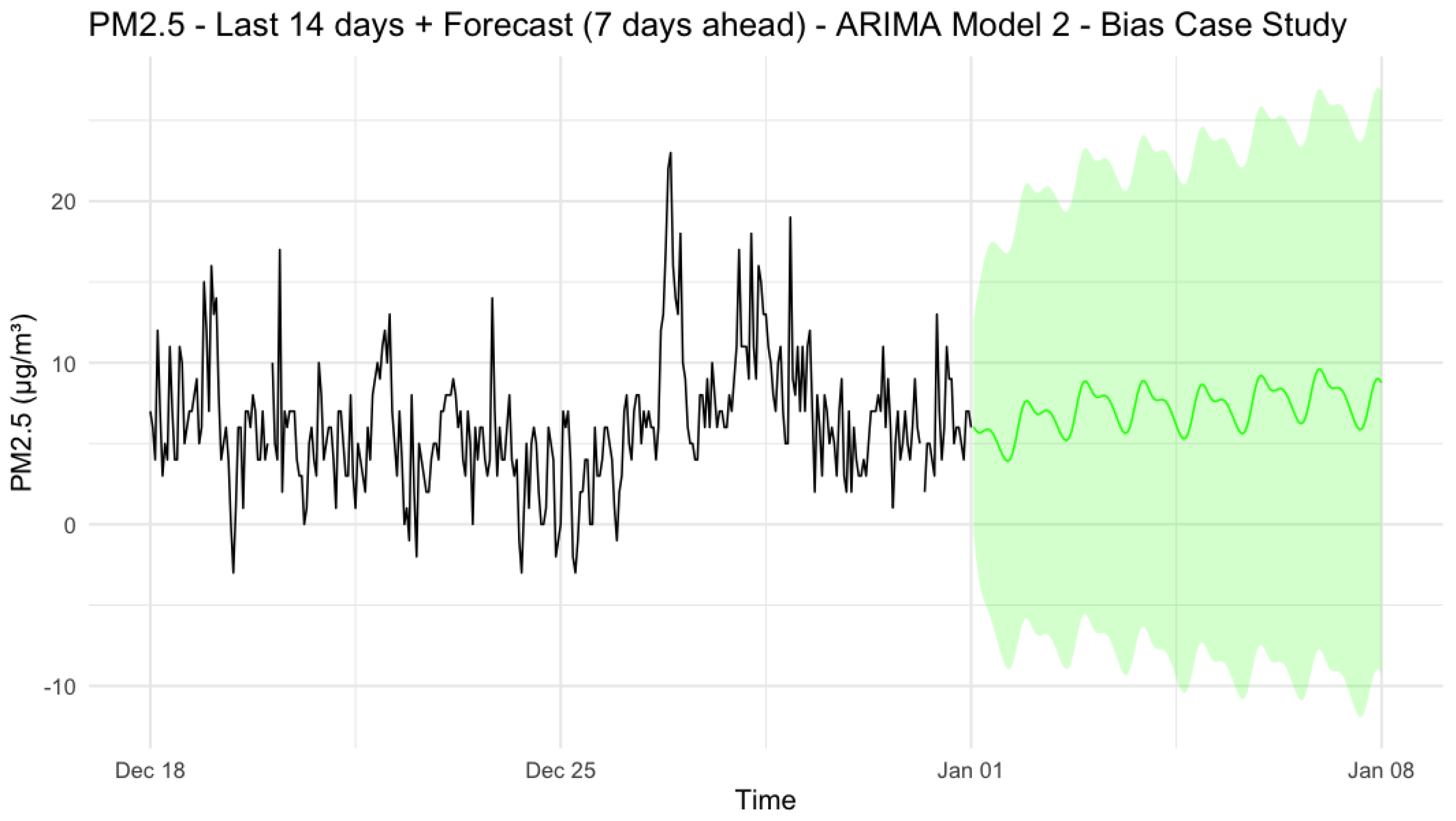
ARIMA models are commonly implemented using open-source packages, such as the ‘forecast’ package in R, which provides functionalities for fitting and forecasting while including rudimentary handling of missing values. In this methodological step, we explored the package’s default imputation mechanisms, particularly the ‘na.interp’ function, which performs basic linear interpolation to assess their influence on ARIMA model performance without external imputation. This approach generated an imputed dataset that enables later evaluation of its effects on model accuracy and potential biases, especially in the results and discussion sections. Table 2 below summarises the error metrics of ARIMA Model 2.
Figure 3 below illustrates the ARIMA Model 2 forecast for 7 days, with the interpolated PM2.5 concentrations in the green line and the actual observed values in the black line, visually confirming the performance of the model on the pre-processed data.

3.2.4. Implementation of Mean/Median Imputation Technique

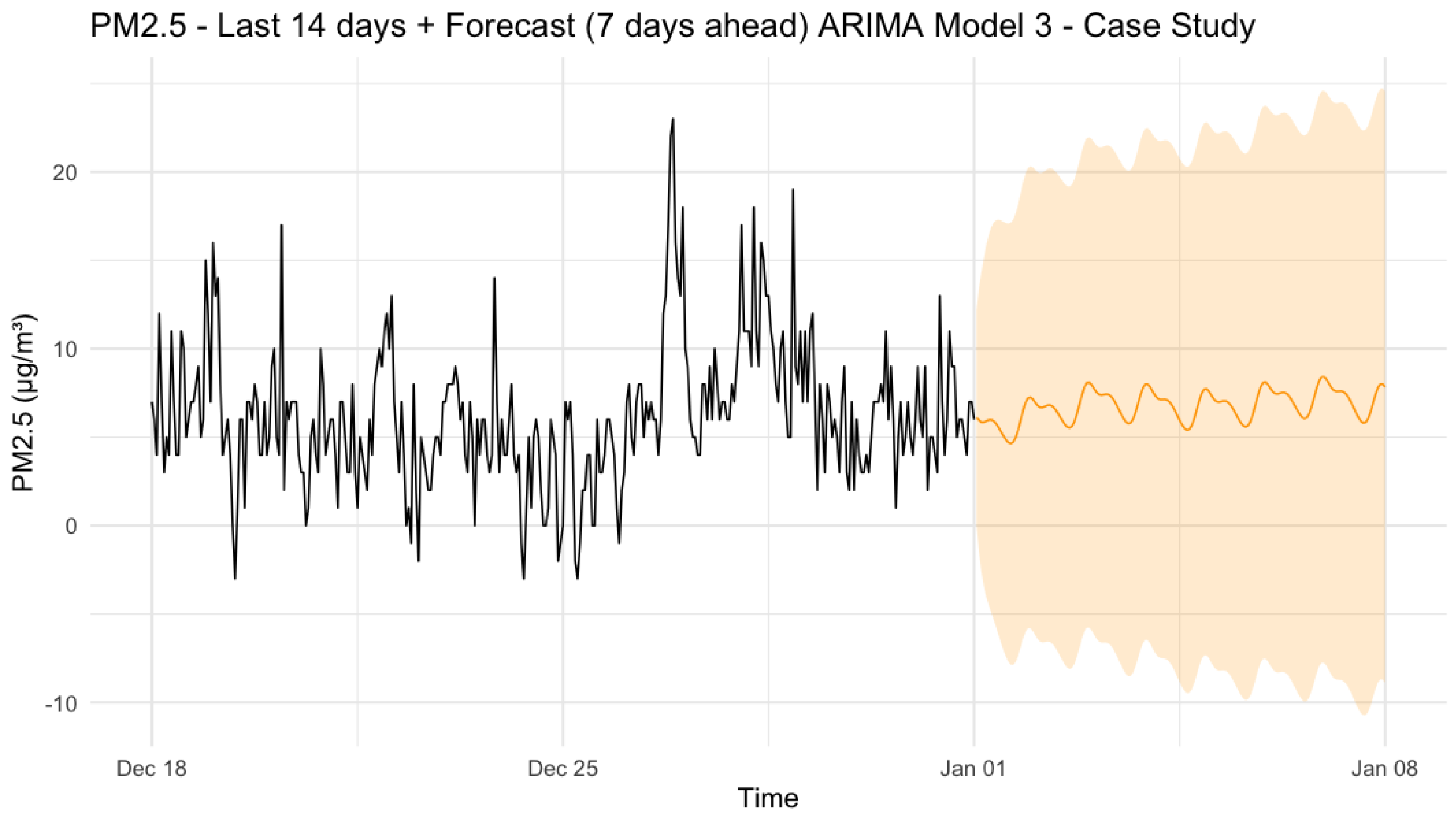
During the implementation of mean or median imputation strategies, missing values in the PM2.5 time series were replaced with the global median of the entire dataset, respectively. This straightforward approach offers a simplistic solution to fill data gaps during the data transformation phase. Subsequently, a new variable was created incorporating these imputed values to facilitate direct comparison with the baseline and other imputed ARIMA Model 1. Table 3 below summarises the error metrics for ARIMA Model 3.
Figure 4 below illustrates the ARIMA Model 3 forecast for 7 days, with the median PM2.5 concentrations added in the orange line and the actual observed values in the black line, visually confirming the improved performance of the model on the pre-processed data.

3.3. Validation Techniques

Given the critical role of imputation in the analysis of time-series data, particularly when dealing with environmental datasets characterised by inherent missing values, precise validation steps are essential to ensure the reliability and precision of subsequent analyses [36]. Taking into account the above implementation steps, this study employs two primary validation methodologies: statistical comparison analysis and visual interpretation analysis. The statistical comparison analysis technique involves a direct quantitative comparison of key performance indicators, such as mean error (ME), root mean square error (RMSE), mean absolute error (MAE), mean absolute scaled error (MASE) and autocorrelation function in leg 1 (ACF1), across different ARIMA models to determine which imputation method yields the most accurate and reliable forecasts. Visual interpretation analysis complements this by qualitatively assessing applied imputation methods through graphical representations, allowing for an intuitive understanding of how each imputation method influences the reconstructed time series and its alignment with baseline patterns.

4. Results & Discussion

In this section, the results will be outlined and explained, reflecting the methodology proposed in Section 3.2. All results were obtained using the open-source tool RStudio with a version of 2025.05.1 in conjunction with the R programming language and the relevant libraries.

4.1. Results

All three ARIMA models have projected different results, a direct quantitative comparison of key performance indicators, such as ME, RMSE, MAE, MASE, and ACF1, across the different ARIMA models to determine which imputation method yields the most accurate and reliable forecasts. Table 4 below summarises the statistical parameters obtained for each model.

4.2. Validation-Based Discussion

Upon examination of the statistical comparative analysis, the ME for all three ARIMA models is close to zero, indicating negligible systematic bias in the predictions. The forecast accuracy improves progressively from ARIMA Model 1 to ARIMA Model 3, and ARIMA Model 3 demonstrates the lowest RMSE and MAE values, thus indicating superior predictive performance. In contrast, scaled accuracy metrics such as MASE favour ARIMA Model 2, while ACF1 shows a marginally better fit for ARIMA Model 3. Overall, while ARIMA Model 3 provides the most accurate forecasts in absolute terms and ARIMA Model 2 minimises bias and relative error, ARIMA Model 1 performs comparatively weaker across most evaluation criteria.
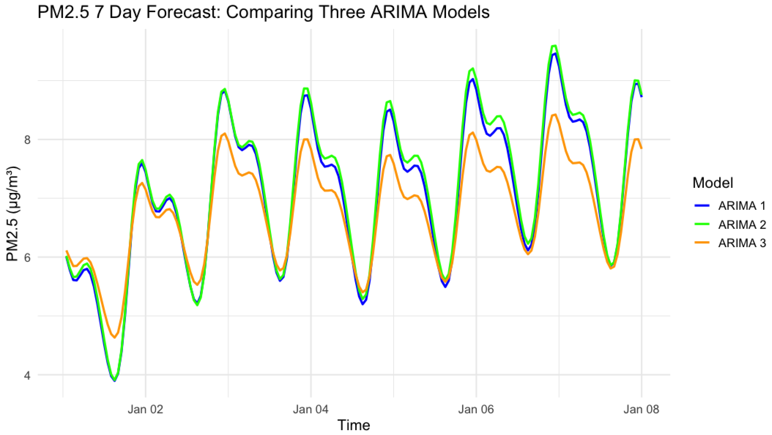
The visual interpretation of Figure 5 presents a comparative analysis of PM2.5 concentrations over a 7-day forecast period for three ARIMA models, illustrating key findings of the study. Figure 5 visualisation displays the baseline data, the linearly interpolated dataset and the median-imputed dataset, allowing a comprehensive assessment of the impact of each imputation strategy on the forecast trajectories compared to the actual observed values. In the visuals, the blue line represents ARIMA Model 1, the green line represents ARIMA Model 2, and the orange line represents ARIMA Model 3.
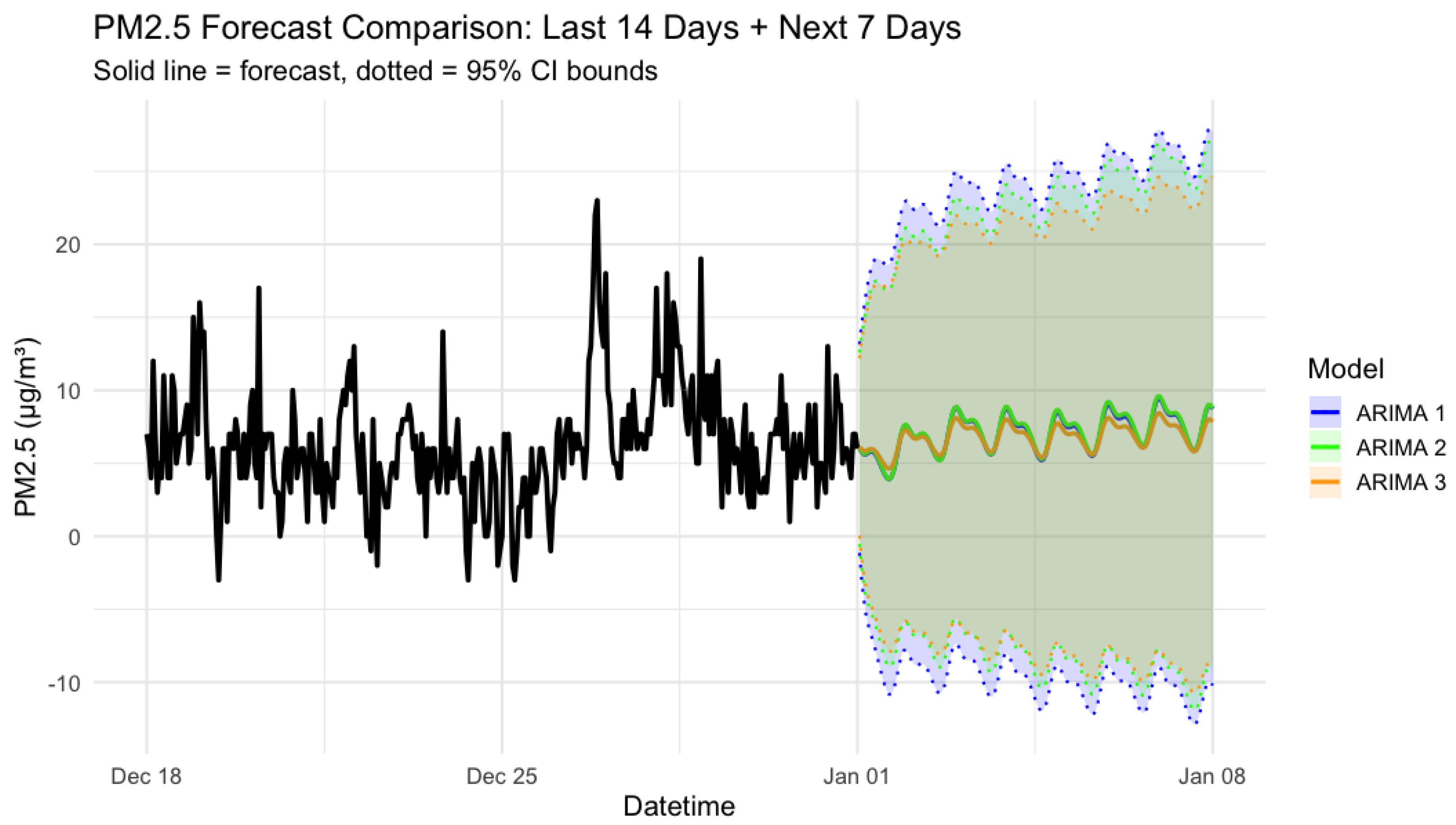
In addition to statistical and visual analysis, a deeper dive is to examine confidence interval bounds (CIBs) between the three ARIMA models to further evaluate the certainty and precision of their predictions across different imputation methods. The visual Figure 6 confirms that the CIBs are narrowest for ARIMA Model 3, indicating improved predictive reliability and reduced uncertainty attributable to the median imputation.
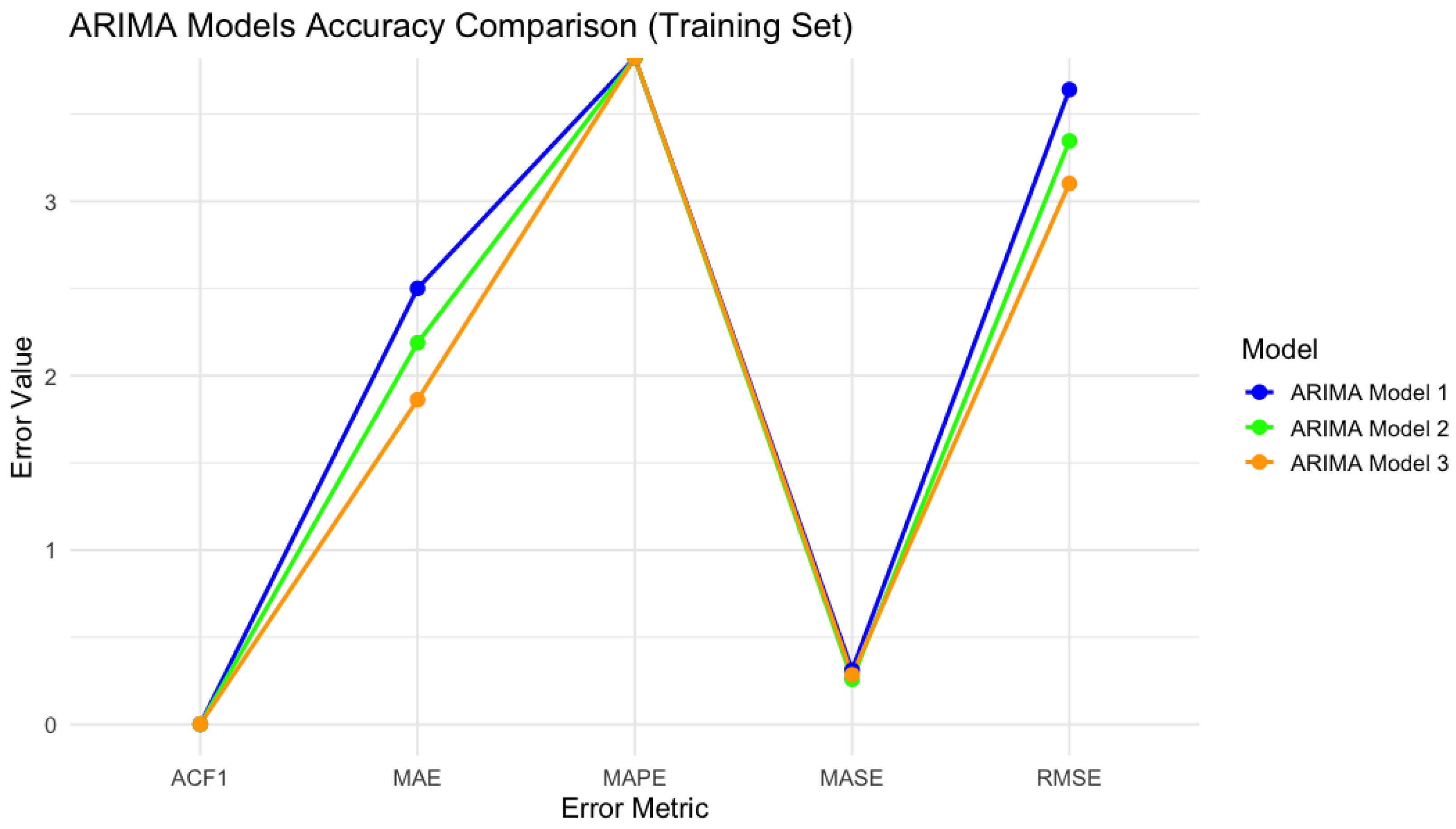
Following the CIB findings in Figure 6, statistically, ARIMA Model 3 has a lower peak (8.4 µg/m3) compared to other ARIMA model peaks (9.6 µg/m3). Finally, another visual graph Figure 7 was generated to illustrate the comparison of error metrics, with a line graph that highlights the variance in ACF1, MAE, MASE, and RMSE values in all three ARIMA models, thus offering an intuitive understanding of the predictive accuracy and bias of each model with respect to the different imputation techniques. In visual form, the blue line represents ARIMA Model 1, the green line represents ARIMA Model 2, and the orange line represents ARIMA Model 3, demonstrating that ARIMA Model 3 consistently exhibits the lowest error metrics across all parameters tested.

5. Conclusions

The paper concludes by highlighting key insights into biases in imputation techniques for advanced data science practices, while showcasing the distinct results from each deployed ARIMA model. In particular, median imputation consistently delivered superior performance, particularly for PM2.5 forecasting, underscoring its effectiveness in handling missing data in environmental time series analysis. Additionally, the findings demonstrate that the imputation techniques applied during the data transformation stage significantly impact the performance of the model compared to the methods used in the later stages of the AQ data analysis. The results of all three ARIMA models illustrate how bias can infiltrate the modelling process. Thus, best practices, such as equitable data aggregation, rigorous validation, model transparency, and appropriate algorithm selection, are essential to mitigate bias and improve predictive accuracy in air quality forecasting. Based on these findings, future research should prioritise the development of a comprehensive air quality bias mitigation framework. This framework would integrate various AQ datasets and pollutants while evaluating an expanded range of imputation techniques to refine bias-reduction strategies and improve work with different forecasting models other than ARIMA and their correlational dependencies. It should also consider the complex interplay between meteorological factors, emission sources, and atmospheric chemistry to improve the robustness and generalisability of air quality forecasts. Additionally, these findings provide a foundational step in generating additional research hypotheses and encourage future research into more advanced imputation strategies and forecasting frameworks within air quality data analysis.

Author Contributions

All authors contributed to the conception and design of the study. Conceptualisation, E.H.; methodology, E.H.; software, E.H.; validation, E.H., Y.L. and A.R.A.; formal analysis, E.H.; investigation, E.H.; resources, E.H.; data curation, E.H.; writing—original draft preparation, E.H.; writing—review and editing, E.H., Y.L. and A.R.A.; visualisation, E.H.; supervision, Y.L. and A.R.A.; project administration, E.H. All authors have read and agreed to the published version of the manuscript.

Funding

This research received no external funding.

Data Availability Statement

The research data has been extracted using an open-source online platform, supported by Air Quality England [33], the online platform allow researchers to pick and select relevant air quality monitoring station, for this instance Wren Close monitoring station was selected for ARIMA modelling.

Acknowledgments

During the preparation of this manuscript/study, the author used RStudio Version 2025.05.1+513 for the purposes of air quality data analysis, transformation, and ARIMA-based statistical modelling. The author also used the Overleaf online platform for the preparation of the paper write-up. The authors have reviewed and edited the output and take full responsibility for the content of this publication.

Conflicts of Interest

The authors declare no conflicts of interest.

Abbreviations

The following abbreviations are used in this manuscript:
AQAir Quality
ARIMAAutoRegressive Integrated Moving Average
PM2.5Fine Particulate Matter 2.5
AQEAir Quality England
DEFRADepartment for Environment, Food & Rural Affairs
UKUnited Kingdom
EUEuropean Union
MEMean Error
RMSERoot Mean Square Error
MAEMean Absolute Error
MASEMean Absolute Scaled Error
ACF1Autocorrelation Function at leg 1
CIBConfidence Interval Bounds
OSOpen-Source
IoTInternet of Things
LAQMLocal Air Quality Management
µg/m3Micrograms per cubic meter (Pollutant Unit)
BAMbeta attenuation monitor

References

  1. Mehmood, K.; Bao, Y.; Cheng, W.; Khan, M.A.; Siddique, N.; Abrar, M.M.; Soban, A.; Fahad, S.; Naidu, R. Predicting the quality of air with machine learning approaches: Current research priorities and future perspectives. J. Clean. Prod. 2022, 379, 134656. [Google Scholar] [CrossRef]
  2. Liu, X.; Ngai, E.C.-H.; Zachariah, D. Scalable Belief Updating for Urban Air Quality Modeling and Prediction. ACM/IMS Trans. Data Sci. 2021, 2, 1–19. [Google Scholar] [CrossRef]
  3. Yan, S.; O’Connor, D.J.; Wang, X.; O’Connor, N.E.; Smeaton, A.F.; Liu, M. Comparative Analysis of Machine Learning-Based Imputation Techniques for Air Quality Datasets with High Missing Data Rates. In 2025 IEEE Symposia on Computational Intelligence for Energy, Transport and Environmental Sustainability (CIETES); IEEE: Piscataway, NJ, USA, 2025; pp. 1–8. [Google Scholar] [CrossRef]
  4. Hua, V.; Nguyen, T.; Dao, M.S.; Nguyen, H.D.; Nguyen, B.T. The impact of data imputation on air quality prediction problem. PLoS ONE 2024, 19, e0306303. [Google Scholar] [CrossRef] [PubMed]
  5. Silibello, C.; D’Allura, A.; Finardi, S.; Bolignano, A.; Sozzi, R. Application of bias adjustment techniques to improve air quality forecasts. Atmos. Pollut. Res. 2015, 6, 928–938. [Google Scholar] [CrossRef]
  6. Hanson, B.; Stall, S.; Cutcher-Gershenfeld, J.; Vrouwenvelder, K.; Wirz, C.; Rao, Y.; Peng, G. Garbage in, garbage out: Mitigating risks and maximizing benefits of AI in research. Nature 2023, 623, 28–31. [Google Scholar] [CrossRef]
  7. Qin, S.; Liu, F.; Wang, J.; Sun, B. Analysis and forecasting of the particulate matter (PM) concentration levels over four major cities of China using hybrid models. Atmos. Environ. 2014, 98, 665–675. [Google Scholar] [CrossRef]
  8. Yan, Z. Comparative Analysis of ARMA and ARIMA Models for Air Quality Prediction. Adv. Eng. Technol. Res. 2025, 14, 1349. [Google Scholar] [CrossRef]
  9. Shaadan, N.; Rahim, N.A.M. Imputation analysis for time series air quality (PM10) data set: A comparison of several methods. In Journal of Physics: Conference Series; IOP Publishing: Bristol, UK, 2019; Volume 1366, p. 012107. [Google Scholar] [CrossRef]
  10. Blair, G.S.; Henrys, P.A.; Leeson, A.; Watkins, J.; Eastoe, E.; Jarvis, S.G.; Young, P.J. Data science of the natural environment: A research roadmap. Front. Environ. Sci. 2019, 7, 121. [Google Scholar] [CrossRef]
  11. Rosales, C.M.; Bratburd, J.R.; Diez, S.; Duncan, S.; Malings, C.; Pant, P. Open air quality data platforms for environmental health research and action. Curr. Environ. Health Rep. 2025, 12, 27. [Google Scholar] [CrossRef]
  12. Dosemagen, S.; Williams, E. Data usability: The forgotten segment of environmental data workflows. Front. Clim. 2022, 4, 785269. [Google Scholar] [CrossRef]
  13. Okafor, N.U.; Alghorani, Y.; Delaney, D. Improving data quality of low-cost IoT sensors in environmental monitoring networks using data fusion and machine learning approach. ICT Express 2020, 6, 220–228. [Google Scholar] [CrossRef]
  14. DEFRA: Department for Environment, Food & Rural Affairs, Guidance. 2026. Available online: https://laqm.defra.gov.uk/guidance/ (accessed on 3 March 2026).
  15. Mikusch, G.; Petz, A.; Steiner, E.; Tabakovic, M.; Tellioglu, H. Environmental data sensing through participatory urbanism. A best-practice analysis and city-administration perspective. GI-Forum-J. Geogr. Inf. Sci. 2023, 11, 3–17. [Google Scholar] [CrossRef]
  16. Mahajan, S. Design and development of an open-source framework for citizen-centric environmental monitoring and data analysis. Sci. Rep. 2022, 12, 14416. [Google Scholar] [CrossRef] [PubMed]
  17. Katie, B. Internet of Things (IoT) for environmental monitoring. Int. J. Comput. Eng. 2024, 6, 29–42. [Google Scholar] [CrossRef]
  18. Kim, T.; Kim, J.; Yang, W.; Lee, H.; Choo, J. Missing value imputation of time-series air-quality data via deep neural networks. Int. J. Environ. Res. Public Health 2021, 18, 12213. [Google Scholar] [CrossRef] [PubMed]
  19. Jaoudé, A.A.; Abou, A.; Qamber, I.S.; Al-Hamad, M.Y.; Turabieh, H.; Sheta, A.; Braik, M.; Kovač-Andrić, E.; Saroha, S.; Aggarwal, S.K.; et al. Forecasting in mathematics: Recent advances, new perspectives and applications. In IntechOpen eBooks; IntechOpen: Rijeka, Croatia, 2020. [Google Scholar] [CrossRef]
  20. Phan, T.-T.-H.; Thi-Thu-Hong, P.H.A.N. Elastic Matching for Classification and Modelisation of Incomplete Time Series. Doctoral Dissertation, Université Paris Sud, Orsay, France, 2018. [Google Scholar]
  21. Ribeiro, S.M.; de Castro, C.L. Missing data in time series: A review of imputation methods and case study. Learn. Nonlinear Model. 2022, 20, 31. [Google Scholar] [CrossRef]
  22. Rahman, N.H.A.; Lee, M.H. Artificial neural network forecasting performance with missing value imputations. IAES Int. J. Artif. Intell. 2020, 9, 33–39. [Google Scholar] [CrossRef]
  23. Hoffman, S. Estimation of prediction error in regression air quality models. Energies 2021, 14, 7387. [Google Scholar] [CrossRef]
  24. Ramadan, M.S.; Abuelgasim, A.; Al Hosani, N. Advancing air quality forecasting in Abu Dhabi, UAE using time series models. Front. Environ. Sci. 2024, 12, 1393878. [Google Scholar] [CrossRef]
  25. Fatima, N.; Yousafzai, S.N.; Nemri, N.; Alsolai, H.; Ebad, S.A.; Sorour, S.; Gu, Y.; Syafrudin, M.; Fitriyani, N.L. Time series AQI forecasting using Kalman-integrated Bi-GRU and Chi-square divergence optimization. Sci. Rep. 2025, 15, 29157. [Google Scholar] [CrossRef]
  26. Safarov, R.; Shomanova, Z.; Nossenko, Y.; Kopishev, E.; Bexeitova, Z.; Kamatov, R. Filling gaps in PM2.5 time series: A broad evaluation from statistical to advanced neural network models. PLoS ONE 2025, 20, e0330211. [Google Scholar] [CrossRef]
  27. Bernacki, J.; Scherer, R. A Comprehensive Review of Data-Driven Techniques for Air Pollution Concentration Forecasting. Sensors 2025, 25, 6044. [Google Scholar] [CrossRef] [PubMed]
  28. Cujia, A.; Agudelo-Castañeda, D.; Pacheco-Bustos, C.; Teixeira, E.C. Forecast of PM10 time-series data: A study case in Caribbean cities. Atmos. Pollut. Res. 2019, 10, 2053–2062. [Google Scholar] [CrossRef]
  29. Libasin, Z.; Wan Mohamed Fauzi, W.S.; Idris, N.A.; Mazeni, N.A. Evaluation of Single Missing Value Imputation Techniques for Incomplete Air Particulates Matter (PM 10) Data in Malaysia. Pertanika J. Sci. Technol. 2021, 29, 3099–3112. [Google Scholar] [CrossRef]
  30. Díaz-González, L.; Trujillo-Uribe, I.; Pérez-Sansalvador, J.C.; Lakouari, N. Handling Missing Air Quality Data Using Bidirectional Recurrent Imputation for Time Series and Random Forest: A Case Study in Mexico City. AI 2025, 6, 208. [Google Scholar] [CrossRef]
  31. Nugroho, H.; Surendro, K. A comprehensive bibliometric analysis of missing value imputation. IEEE Access 2024, 12, 14819–14846. [Google Scholar] [CrossRef]
  32. Arnaut, F.; Đurđević, V.; Kolarski, A.; Srećković, V.A.; Jevremović, S. Improving air quality data reliability through bi-directional univariate imputation with the random forest algorithm. Sustainability 2024, 16, 7629. [Google Scholar] [CrossRef]
  33. AQE: About Air Quality England. 2020. Available online: https://www.airqualityengland.co.uk/about (accessed on 1 March 2026).
  34. Choudhary, A.; Kumar, P.; Sahu, S.K.; Pradhan, C.; Singh, S.K.; Gašparović, M.; Shukla, A.; Singh, A.K. Time Series Simulation and Forecasting of Air Quality Using In-situ and Satellite-Based Observations Over an Urban Region. Nat. Environ. Pollut. Technol. 2022, 21, 1137–1148. [Google Scholar] [CrossRef]
  35. Conner, A.; Hosking, S.; Lloyd, J.; Rao, A.; Shaddick, G.; Sharan, M. Tackling Climate Change with Data Science and AI; Zenodo: Geneva, Switzerland, 2023. [Google Scholar] [CrossRef]
  36. van der Aalst, W.M.; Bichler, M.; Heinzl, A. Responsible data science. Bus. Inf. Syst. Eng. 2017, 59, 311–313. [Google Scholar] [CrossRef]
Figure 1. The figure above depicts the prevalence of missing data in PM2.5 concentrations, indicating that 12,664 out of 43,824 hourly measurements are absent, equivalent to a substantial missing-ness rate of 28.9%.
Algorithms 19 00449 g001
Figure 2. Figure above illustrates 7-day future forecasting of PM2.5 concentration using ARIMA Model 1.
Algorithms 19 00449 g002
Figure 3. Figure above illustrates 7-day future forecasting of PM2.5 concentration using ARIMA Model 2.
Algorithms 19 00449 g003
Figure 4. Figure above illustrates 7-day future forecasting of PM2.5 concentration using ARIMA Model 3.
Algorithms 19 00449 g004
Figure 5. Figure above illustrates a comparison chart of all three ARIMA models.
Algorithms 19 00449 g005
Figure 6. A visual chart comparing three ARIMA models with 95% CIB.
Algorithms 19 00449 g006
Figure 7. A visual chart comparing error metrics for three ARIMA models and shows the statistical difference between each error value.
Algorithms 19 00449 g007
Table 1. Key breakdown of ARIMA Baseline Model 1 output.
Error MetricModel Score
Mean Error (ME)0.002
Root Mean Square Error (RMSE)3.64
Mean Absolute Error (MAE)2.50
Mean Absolute Scaled Error (MASE)0.29
Autocorrelation Function at leg 1 (ACF1)0.001
Residual Standard Deviation (Sigma2)13.27
Table 2. Key breakdown of ARIMA Baseline Model 2 output.
Error MetricModel Score
Mean Error (ME)0.00
Root Mean Square Error (RMSE)3.35
Mean Absolute Error (MAE)2.5
Mean Absolute Scaled Error (MASE)0.25
Autocorrelation Function at leg 1 (ACF1)0.0007
Residual Standard Deviation (Sigma2)11.21
Table 3. Key breakdown of ARIMA Baseline Model 3 output.
Error MetricModel Score
Mean Error (ME)0.00
Root Mean Square Error (RMSE)3.10
Mean Absolute Error (MAE)1.86
Mean Absolute Scaled Error (MASE)0.28
Autocorrelation Function at leg 1 (ACF1)0.001
Residual Standard Deviation (Sigma2)9.62
Table 4. Statistical analysis of all three ARIMA models outputs.
Error MetricARIMA 1ARIMA 2ARIMA 3
ME0.0019491250.0000844−0.0003585713
RMSE3.6403863.3460553.101502
MAE2.5003212.1879551.861751
MASE0.29343550.25863010.2842862
ACF10.0011947340.00075302990.001449699
Disclaimer/Publisher’s Note: The statements, opinions and data contained in all publications are solely those of the individual author(s) and contributor(s) and not of MDPI and/or the editor(s). MDPI and/or the editor(s) disclaim responsibility for any injury to people or property resulting from any ideas, methods, instructions or products referred to in the content.