VISR-CNN: A Dual-Stream Framework for Meteorological Visibility Estimation via Multi-Scale Transmission Attention and Spectral Gating

Abstract

Accurate meteorological visibility estimation is vital for transportation safety and environmental monitoring. However, modeling the inherent nonlinear spatial and spectral degradations in hazy environments remains challenging. While recent Large Vision-Language Models (LVLMs) offer strong scene understanding, they lack the regression precision required for visibility estimation. In this paper, we propose the Visibility-Aware Refined CNN (VISR-CNN), a dual-stream architecture that synthesizes local spatial cues with global frequency-domain signatures. The model integrates a Multi-Scale Transmission Attention (MSTA) module, which uses parallel dilated convolutions to estimate atmospheric transmission, and a Global Frequency Branch that utilizes 2D Real Fast Fourier Transforms (RFFT) with Spectral Gating to quantify visibility-dependent blurring. A progressive training strategy is introduced to decouple spectral and spatial optimization, and a physics-informed loss function is designed to supervise numerical regression while enforcing a monotonic ranking constraint consistent with physical light-attenuation laws. Results on the HKCHC-VD dataset show that VISR-CNN achieves state-of-the-art performance (MAE: 1.54 km; RMSE: 2.31 km), representing a 13.0% improvement over VisNet. Further evaluations on the CP1 and SWH datasets confirm robust generalization, reducing overall MAE by 21% and 20%, respectively, compared with the hybrid ResNeXt-50 + ViT model. Notably, in safety-critical range (0–10 km), VISR-CNN reduces RMSE for the HKCHC-VD, CP1, and SWH datasets by approximately 55%, 64%, and 71%, respectively, when compared with VisNet. These findings demonstrate the superiority of specialized, physics-grounded architectures over general-purpose LVLMs for high-precision meteorological regression.

1. Introduction

Atmospheric visibility is a critical meteorological parameter that directly impacts the safety and efficiency of transportation systems, including aviation, maritime navigation, and autonomous driving. The visual quality degradation caused by aerosols, which is usually manifested as fog, haze, or smog, results in reduced reflected light and increased atmospheric light scattering [1,2,3]. These factors lead to a decrease in contrast and color fidelity. Therefore, accurate and real-time estimation of visibility distance is crucial for intelligent monitoring systems. While traditional visibility measurements rely on expensive hardware such as transmissometers or scatterometers, the deployment of such equipment is often sparse and costly [4]. Consequently, computer vision-based methods that estimate meteorological visibility using only a single image have attracted significant research attention as a scalable and cost-effective alternative.

Early computer vision approaches for visibility estimation relied heavily on hand-crafted priors and physical models derived from Koschmieder’s law. The Dark Channel Prior (DCP) by He et al. [1], demonstrated that haze density could be approximated by analyzing the statistics of the lowest intensity channel in local patches. Nayar and Narasimhan [2,3] pioneered single-image visibility estimation by analyzing the relationship between atmospheric veil and scene radiance, establishing the theoretical foundation for subsequent learning-based methods. Robert and Michael [5] proposed an automated visibility detection algorithm utilizing camera imagery based on Sobel edge detection and normalized edge extraction. While the method in [5] exhibits limitations when visibility ranges fall below 400 m, our proposed VISR-CNN addresses this by utilizing continuous spectral analysis with regression, which remains effective even in sub-kilometer conditions. Then, research transitioned toward model-driven methods. Raouf et al. [6] proposed a model-driven approach for visibility estimation based on the mapping between the contrast distribution of an image and its visibility. This method is effective in conditions with high visibility (approximately 5000 m), but the error is greater in conditions with low visibility. Lo et al. [7] applied multi-support vector regression for meteorological visibility estimation, demonstrating how traditional machine learning techniques could be adapted to this problem with promising results. Nevertheless, these prior-based methods often rely on idealized assumptions regarding atmospheric homogeneity, which frequently fail in complex, real-world scenarios involving uneven lighting or heterogeneous haze distribution.

The advent of deep learning has shifted the paradigm from manual feature engineering to data-driven representation learning. Yan et al. [8] proposed a discrete label distribution learning module to predict visibility within discrete ranges (e.g., “Low,” “Mid,” and “High”). However, such categorical approaches often fail to capture the full nuance of continuous visibility changes. Cai et al. [9] proposed DehazeNet, demonstrating that Convolutional Neural Networks (CNNs) can effectively learn the mapping between hazy images and corresponding scene clarity. Palvanov and Cho [10] introduced VisNet, a deep integrated CNN for visibility forecasting. Furthermore, a hybrid neural network was proposed in [11] utilizing localized image entropy and image-based features as inputs. Current state-of-the-art methods continue to push the boundaries of accuracy [12,13]. Narksri et al. [13] proposed a method for estimating visibility using 3D point clouds and high-definition road maps. Additionally, an end-to-end CNN framework, the Deep Multihead Regression Network (DMRVisNet), was introduced in [14] for pixel-wise visibility estimation, while a landmark-based ANN method [15] was proposed to utilize the features of distinct landmark objects. However, these methods operate primarily in the spatial domain and generally struggle to generalize under diverse weather conditions.

The success of modern visibility estimation models often depends on the strength of the underlying feature extractor. The introduction of Residual Networks (ResNet) [16] revolutionized deep architectures by allowing gradients to flow through deeper networks without vanishing, thereby enabling the extraction of high-level semantic features. Building upon this, ResNeXt [17] introduced a new dimension called “cardinality” to improve classification accuracy and robustness. While ResNet and ResNeXt backbones excel at capturing spatial object details, visibility estimation presents a unique challenge. In fact, haze is not merely a localized object feature but a global degradation that effectively acts as a low-pass filter, attenuating high-frequency texture details across the entire image. Standard CNNs, which focus primarily on local spatial convolutions, often struggle to explicitly model this global frequency degradation, leading to suboptimal performance under varying atmospheric density conditions.

To address the limitations of purely spatial feature extraction, recent research has begun to explore the potential of the frequency domain. Moorthy and Bovik [18] developed a blind image quality assessment method in the Discrete Cosine Transform (DCT) domain to detect compression artifacts and blurring. These phenomena are directly related to visibility estimation due to the reduction of contrast and edge sharpness. Xu et al. [19] further demonstrated that frequency-domain processing can enhance robustness against common image corruptions, showing that learning in the spectral domain offers computational advantages and improved generalization. Mittal et al. [20] established that no-reference image quality assessment in the spatial domain could be significantly enhanced by incorporating frequency-domain features, providing theoretical support for dual-domain architecture. In [21], the authors indicated that the use of frequency-domain analysis is indispensable for robust visibility estimation.

By transforming images via the Fast Fourier Transform (FFT), it becomes possible to isolate the spectral components most affected by atmospheric scattering [22]. The choice of the FFT over alternative transformations, such as Wavelet Transform (WT), is motivated by the global nature of atmospheric degradation. While WT excels at localizing non-stationary features, FFT provides a holistic power spectrum that allows our framework to more effectively quantify visibility-dependent contrast attenuation across the entire field of view. However, integrating frequency-domain analysis with spatial backbones presents a significant optimization challenge. Multi-modal networks often suffer from training instability, where one branch, typically the dominant spatial backbone, overpowers the gradient flow. This prevents auxiliary branches from learning meaningful representations and necessitates a robust training curriculum to ensure balanced feature integration.

Existing methodologies have been summarized in

Table 1. Comparison of existing visibility estimation methodologies and identified research gaps.

Methodology	Focus/Core Mechanism	Critical Research Gaps & Limitations
Traditional Physical Models [1,2,3,5]	Dark Channel Prior (DCP); Koschmieder’s Law; Edge detection.	Relies on idealized atmospheric homogeneity; fails in complex urban scenes with heterogeneous haze or uneven lighting.
Statistical & ML Methods [6,7]	Contrast mapping; Multi- SVR.	Effective for high visibility (~5000 m) but exhibits high error margins in safety-critical low-visibility ranges (<400 m).
Spatial-Only Deep Learning [8,9,10,11,12,13,14,15]	CNNs (DehazeNet, VisNet); 3D point clouds; Discrete labeling.	Operates primarily in the spatial domain; local convolutions often struggle to generalize across diverse global atmospheric degradation patterns.
Advanced Backbones [16,17]	ResNet; ResNeXt (Residual & Cardinality-based learning).	Optimized for object semantic extraction; lacks explicit mechanisms to model haze as a global frequency low-pass filter.
Early Dual- Domain Fusion [18,19,20,21]	Hybrid CNN and DCT/FFT features; frequency-domain quality assessment.	Lacks adaptive frequency filtering (Spectral Gating) and physics-informed constraints to prevent branch interference.

. Traditional physical models [1,2,3,5] and statistical methods [6,7] are often constrained by idealized atmospheric assumptions, leading to high error margins in safety-critical low-visibility conditions. Conversely, while deep learning approaches [8,9,10,11,12,13,14,15] and advanced backbone [16,17] excel at hierarchical feature extraction, they operate primarily in the spatial domain and lack explicit mechanisms to model haze as a global frequency degradation. Furthermore, early attempts at dual-domain fusion [18,19,20,21] do not utilize adaptive frequency filtering or physical consistency constraints, often resulting in branch interference.

In this paper, we propose a novel framework, the Visibility-Aware Refined CNN (VISR-CNN), which effectively fuses a ResNeXt-50 spatial backbone with a dedicated Global Frequency Branch for visibility estimation. Specifically, let the input hazy image be denoted as $\mathbf{I}\in {\mathbb{R}}^{3\times H\times W}$. We define the visibility estimation task as learning a mapping function $\mathcal{F}:\mathbf{I}\to V$, where $V\in {\mathbb{R}}^{+}$ represents the meteorological visibility distance. Following the Koschmieder Law, the relationship between the observed intensity $\mathbf{I}$ and the scene radiance $\mathbf{J}$ is modeled as:

$$\mathbf{I}\left(x\right)=\mathbf{J}\left(x\right)e^{-B·d\left(x\right)}+A\left(1-e^{-B·d\left(x\right)}\right)$$

(1)

where $B$ is the atmospheric extinction coefficient, $d\left(x\right)$ is the scene depth, and $A$ is the global atmospheric light. Our VISR-CNN is designed to implicitly estimate $B$ by leveraging both spatial attenuation and global frequency distributions, grounded in the Koschmieder relation $V\approx 3.912/B$.

The novelty of VISR-CNN lies in its specialized architectural alignment with the physics of atmospheric scattering, distinguishing it from general-purpose multi-modal models in three ways:

• Physics-Informed Frequency Selection: Unlike prior works that utilize the entire spectral domain, our Spectral Gating (SG) module employs learnable masks to adaptively isolate the low-to-mid frequency components that contain structural silhouettes, effectively filtering out high-frequency atmospheric noise.
• Multi-Scale Transmission Attention (MSTA): We introduce a transmission-aware attention mechanism that specifically targets multi-scale contrast degradation—a primary indicator of visibility loss that standard spatial-only attention mechanisms often fail to capture.
• Monotonic Ranking Supervision: While existing studies treat visibility as a standard regression task, we integrate a Monotonic Ranking Loss that enforces the ordinal physical constraints of light attenuation, ensuring that the model’s predictions remain physically consistent even in data-sparse low-visibility conditions.

Experimental results across diverse datasets (HKCHC-VD, CP1, and SWH) demonstrate that our VISR-CNN framework significantly outperforms both traditional specialized architectures and state-of-the-art vision-language models.

2. Methodology

In this study, we propose the Visibility-Aware Refined CNN (VISR-CNN), a dual-branch deep learning architecture designed to estimate atmospheric visibility from single images. The proposed framework integrates spatial feature extraction with frequency domain analysis to effectively model the degradation caused by haze. The overall architecture consists of a spatial branch equipped with Multi-Scale Transmission Attention (MSTA), a global frequency branch utilizing spectral gating, and a physics-informed loss function.

2.1. Data Characteristics, Preprocessing and Augmentation

The datasets utilized in this study are captured from high-resolution meteorological cameras situated at high-vantage observation points. These vantage points provide a vast depth of field that encompasses both near-field structures and the distant horizon, capturing a wide range of atmospheric extinction levels over thousands of single frames. This spatial complexity and data scale require a robust data pipeline to ensure the model generalizes across varied environmental conditions. Further technical details regarding the datasets are provided in Section 2.4.3.

To ensure robust model training, the input images are preprocessed using a custom data pipeline. All images are resized to a fixed resolution of 224 × 224 pixels. We apply standard normalization using the mean and standard deviation of the ImageNet dataset (μ = [0.485, 0.456, 0.406], σ = [0.229, 0.224, 0.225]).

During the training phase, a comprehensive data augmentation strategy is employed to mitigate overfitting and improve the generalization capabilities of the model across diverse environmental conditions. The spatial augmentations include random rotation, where images are rotated by an angle sampled uniformly from [−15°, 15°], and random resized cropping. The cropping module extracts a region with a random scale factor between 0.8 and 1.0 of the original area before resizing it back to the target input dimensions. Furthermore, to prevent the network from memorizing specific lighting conditions and to explicitly simulate the photometric effects of atmospheric degradation, photometric augmentation is introduced via color jittering. Specifically, the brightness, contrast, and saturation of the training images are randomly adjusted by a factor of up to 20% (±0.2). Atmospheric haze naturally acts as a veil that reduces contrast and mutes color saturation. Therefore, randomly perturbing these specific parameters forces the model to rely on underlying structural and frequency-domain features rather than superficial pixel intensities, which significantly enhances its robustness in real-world meteorological scenarios.

2.2. Network Architecture

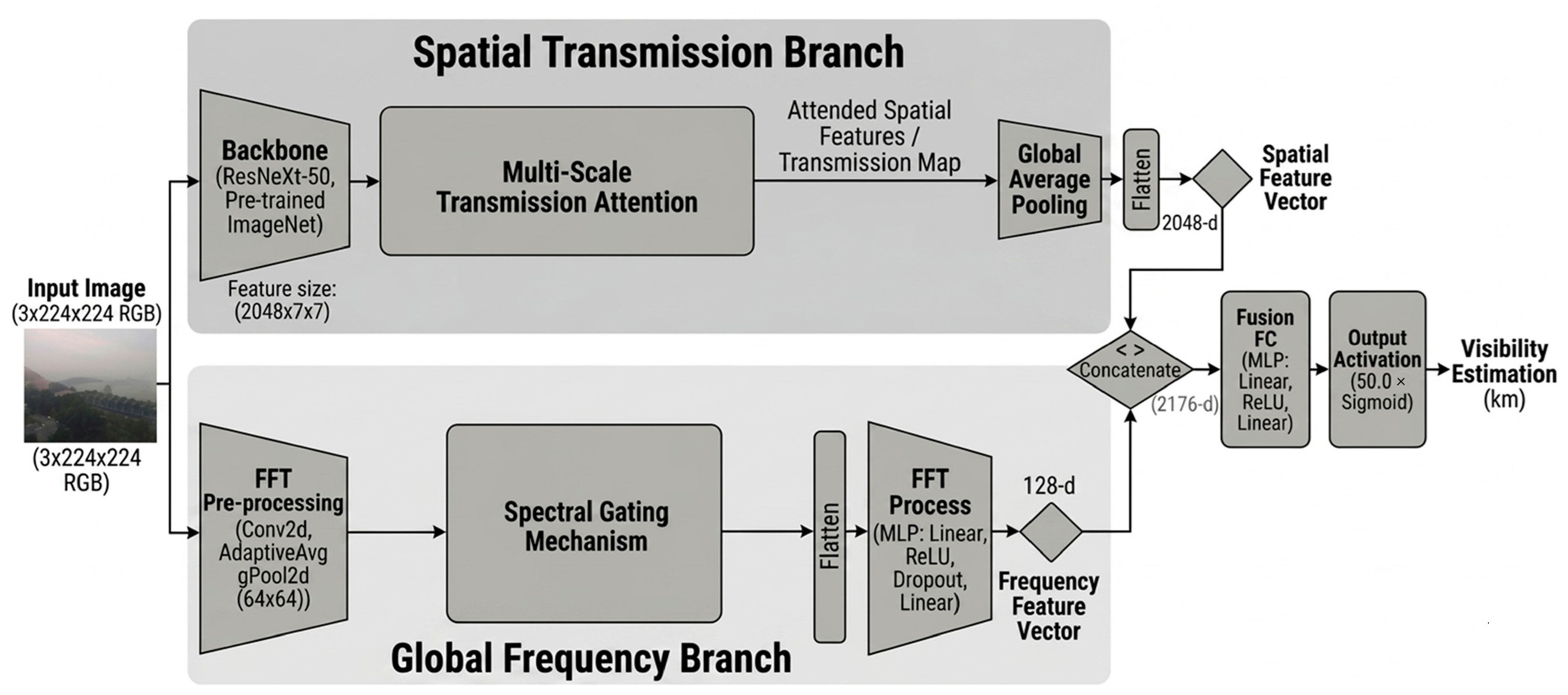
The proposed VISR-CNN architecture with progressive training is a dual-stream framework designed specifically for visibility estimation from single RGB images. As illustrated in Figure 1, the model processes input images through two complementary pathways, including a Global Frequency Branch that leverages the Fast Fourier Transform (FFT) with a spectral gating mechanism and a Spatial Transmission Branch based on convolutional neural networks (CNNs) incorporating the Multi-Scale Transmission Attention (MSTA) module. The output features from both branches are concatenated and subsequently input to a fully connected regression head to predict the scalar visibility value. Furthermore, a progressive training strategy is employed during the training process to ensure stable convergence and a balanced contribution from both branches.

2.2.1. Spatial Transmission Branch

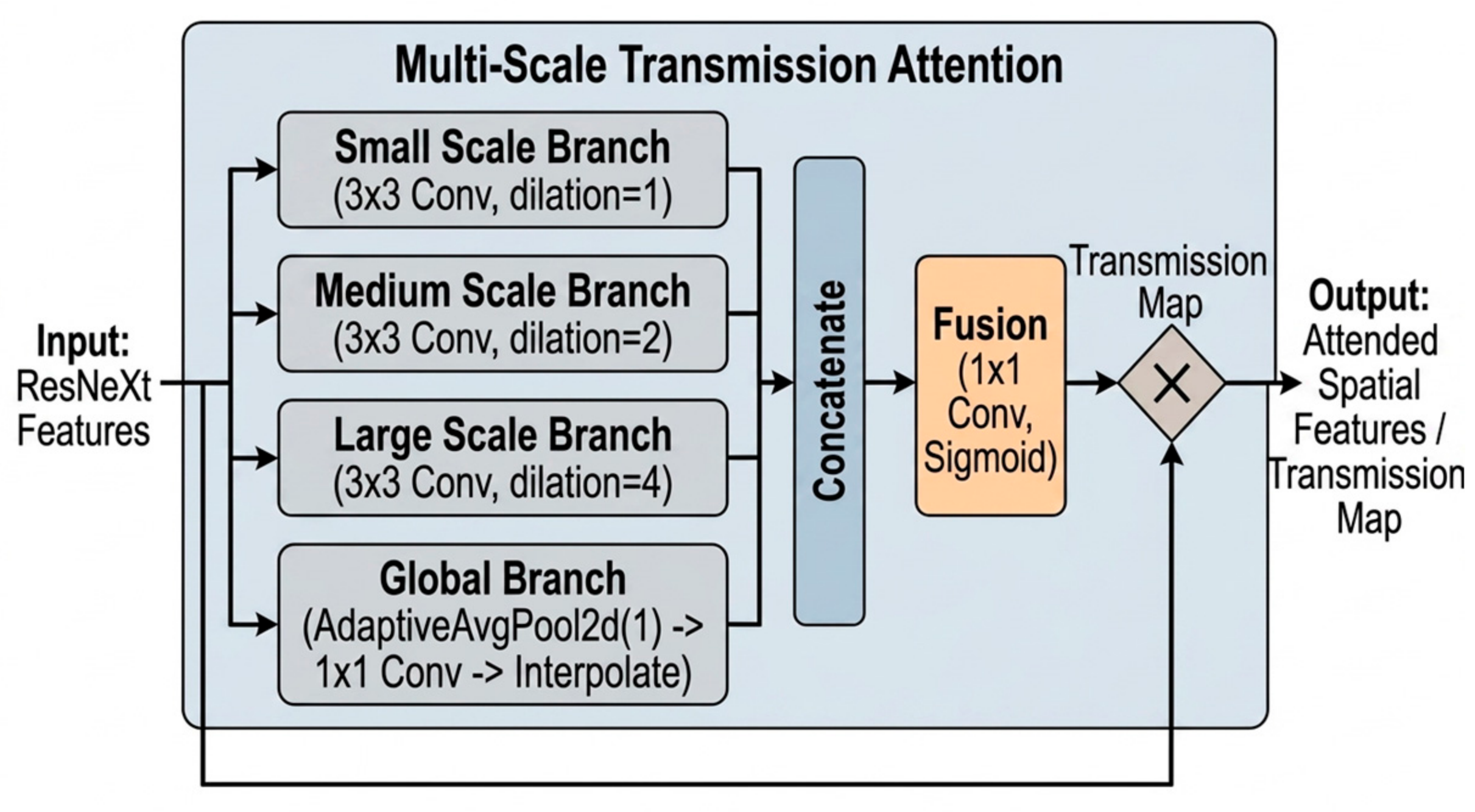
The Spatial Transmission Branch is designed to capture local haze density and structural details. We utilize a ResNeXt-50 backbone, which is pretrained on ImageNet and truncated before the final classification layers. To explicitly model the physics of haze, we introduce a Multi-Scale Transmission Attention (MSTA) module that operates on the feature maps extracted by the backbone. This module employs parallel convolutional branches with varying dilation rates to capture context at different scales. Specifically, inspired by DeepLabv3 [23] and DeepLabv3+ [24] which were used for semantic segmentation task, the architecture integrates a small-scale branch using a 3 × 3 convolution with a dilation rate of d = 1, a medium-scale branch with d = 2, and a large-scale branch with d = 4. Additionally, a global-scale branch is incorporated using adaptive average pooling followed by a 1 × 1 convolution and bilinear upsampling, which is as shown in Figure 2.

By employing dilation rates of $d\in \left\{\mathrm{1,2},4\right\}$, the module effectively captures a hierarchical representation of atmospheric degradation. The small-scale branch (d = 1) focuses on preserving high-frequency edges and local textures of foreground objects that are not obscured by haze. Conversely, the medium branch (d = 2) helps the model recognize mid-range structures, while the large-scale (d = 4) and global branches capture the overall brightness and desaturation of colors that occur across the entire scene. This hierarchical approach enables the model to perceive the gradual attenuation of light across distant landmarks, which is similar to the key cues utilized in human visual perception.

The inclusion of the global-scale branch serves as a scene-wide intensity descriptor by applying global average pooling, which is subsequently upsampled and fused with the spatial branches. The outputs of these branches are concatenated and integrated via a 1 × 1 convolutional layer followed by a sigmoid activation function to generate a transmission map, $\mathbf{T}\left(x\right)$. This allows the generated transmission map $\mathbf{T}\left(x\right)$ to be conditioned not only on local contrast but also on the overall luminance and haze saturation of the entire frame. This map acts as an attention mechanism, weighting the input features ${\mathbf{F}}_{in}$ via element-wise multiplication:

$${\mathbf{F}}_{out}={\mathbf{F}}_{in}\odot \mathbf{T}\left(x\right)$$

(2)

where ⊙ denotes the Hadamard product. In this formulation, $\mathbf{T}\left(x\right)$ suppresses features in regions characterized by heavy haze using low transmission values, while amplifying features in clearer regions where structural integrity is high. This selective weighting ensures that the subsequent regression layers prioritize high-fidelity visual cues over noise-prone hazy pixels. Finally, the refined feature map ${\mathbf{F}}_{out}$ is processed through a Global Average Pooling (GAP) layer to produce a 2048-dimensional spatial feature vector, which encapsulates the depth-dependent visual information necessary for accurate visibility distance estimation.

2.2.2. Global Frequency Branch

Atmospheric haze physically manifests as a spatial low-pass filter. According to the atmospheric optics model, the observed image $I\left(x,y\right)$ can be viewed as the convolution of a clear scene radiance $J\left(x,y\right)$ with a point spread function $h\left(x,y\right)$ representing the scattering effect: $I=J\ast h$. By the Convolution Theorem, this relationship becomes a point-wise product in the frequency domain:

$$F\left(I\right)=F\left(J\right)·H$$

(3)

where $H$ represents the Modulation Transfer Function (MTF) of the atmosphere. Haze attenuates high-frequency components that represent sharp edges and fine textures, leading to a decrease in MTF.

To capture this global spectral degradation, we introduce a dedicated frequency branch. The input image is first processed by a shallow convolutional pre-processor using a 3 × 3 kernel with 32 channels, which extracts spectral-relevant features while reducing the computational load for the transform. It is noted that 3 × 3 kernel size is selected based on VGGNet [25] design principle, which prioritizes small kernels to extract features while maintaining a compact parameter footprint. The output ${\mathbf{I}}_{feat}$ is downsampled via adaptive average pooling to a fixed 64 × 64 grid to ensure consistent frequency resolution regardless of input size. We then transform the feature map into the frequency domain using the two-dimensional Real Fast Fourier Transform (RFFT_2D) [26]:

$$\mathbf{F}\left(u,v\right)=RFF{T}_{2D}\left({\mathbf{I}}_{feat}\left(x,y\right)\right)$$

(4)

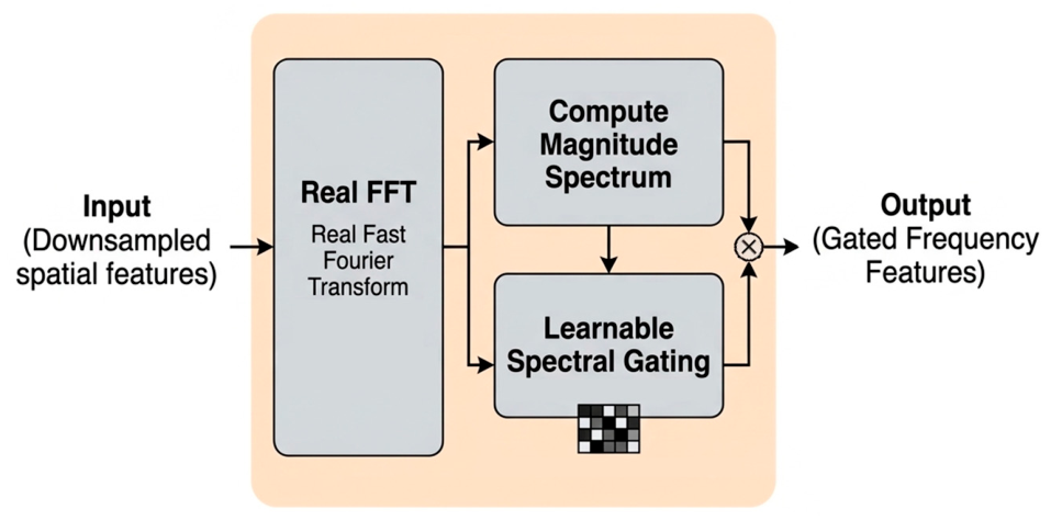
Since the RFFT exploits Hermitian symmetry, it produces a compact representation of size 64 × 33. To allow the network to autonomously identify which frequency bands are most indicative of visibility, such as distinguishing between structural edges and atmospheric noise, we employ a spectral gating mechanism. This involves a learnable complex weight parameter ${\mathbf{W}}_s$ and a bias ${\mathbf{b}}_s$, passed through a sigmoid function to create a spectral mask ${\mathbf{M}}_{freq}$, both of which are optimized during training. The gate is applied to the magnitude of the spectrum:

$${\mathbf{F}}_{gated}\left(u,v\right)=\left|\mathbf{F}\left(u,v\right)\right|\odot {\mathbf{M}}_{freq}$$

(5)

where $\left|\mathbf{F}\left(u,v\right)\right|$ denotes the magnitude of the complex Fourier coefficients and the spectral mask ${\mathbf{M}}_{freq}$ is defined as:

$${\mathbf{M}}_{freq}=\sigma \left({\mathbf{W}}_s\ast \left|\mathbf{F}\left(u,v\right)\right|+{\mathbf{b}}_s\right)$$

(6)

where $\sigma \left(\cdot \right)$ is the Sigmoid function that constrains the mask values to the range (0, 1). The gated magnitude spectrum is flattened into a vector and passed through a specialized multi-layer perceptron (MLP). This MLP utilizes dropout with a probability of $\left(p=0.3\right)$ to prevent overfitting on specific frequency artifacts, ultimately producing a 128-dimensional frequency feature vector that encodes the global structural integrity of the scene. The Real FFT and gating processes are illustrated in Figure 3.

2.2.3. Feature Fusion and Output

The final estimation stage requires the synthesis of two distinct perspectives, consisting of the spatial distribution of haze from the ResNeXt-50 branch and the global spectral degradation from the frequency branch. We employ a late fusion strategy to combine these modalities. The 2048-dimensional spatial vector refined by the MSTA is concatenated with the 128-dimensional frequency vector, resulting in a joint feature representation $\mathit{z}$ of 2176 dimensions. The fusion vector is processed by a regression MLP consisting of a linear layer that projects the 2176-dimensional features into a 512-dimensional hidden space, with ReLU activation [27] to introduce non-linearity for modeling complex atmospheric interactions, and an output layer that maps the hidden features to a single scalar value. Also, by forcing the high-dimensional fused features through a narrower hidden layer, the network is compelled to discard redundant spatial-spectral noise and retain only the most salient latent representations necessary for visibility regression.

The final output is the estimated meteorological visibility, which is constrained to the range [0, $V_{max}$] km using a scaled sigmoid function:

$$V_{pred}=V_{max}\cdot \sigma \left(\mathbf{W}\mathbf{z}+\mathbf{b}\right)$$

(7)

where $\mathbf{W}$ and $\mathbf{b}$ are the learnable weight matrix and bias vector of the final output layer respectively, with $\sigma \left(\cdot \right)$ being the Sigmoid function, and $V_{max}=50.0 \mathrm{k}\mathrm{m}$, which is the physical upper bound of the sensors. By feature fusion, we ensure the model maintains high sensitivity in low-visibility ranges, specifically between 0 and 10 km, where accuracy is most critical for transport safety, while effectively saturating as conditions approach clear-sky limits.

2.3. Physics-Informed Loss Function

The training objective is defined by a composite loss function designed to balance absolute numerical accuracy with the relative structural consistency of the visibility predictions. Traditional regression losses often struggle with meteorological datasets where sensor noise and non-linear haze distributions can lead to local minima. To mitigate this, we propose a physics-informed objective:

$$L_{total}=L_{reg}+\beta L_{rank}$$

(8)

where $\beta$ is a weighting hyperparameter set to 0.05. This value was empirically determined to balance the physical constraints of the ranking loss without dominating the primary regression objective.

2.3.1. Hybrid Regression Loss

The regression component combines Mean Squared Error (MSE) and Mean Absolute Error (MAE) to create a robust optimization surface. The MSE term ($l_2$ norm) penalizes large deviations heavily, facilitating rapid convergence during the early stages of training. Conversely, the MAE term ($l_1$ norm) provides a constant gradient for small errors, making the model more resilient to outliers and sensor noise inherent in visibility ground truth data.

$$L_{reg}={‖V_{pred}-V_{gt}‖}_2^2+{‖V_{pred}-V_{gt}‖}_1$$

(9)

where $V_{pred}$ and $V_{gt}$ are the predicted visibility value and the ground truth visibility value, respectively.

2.3.2. Monotonic Ranking Loss

A critical challenge in visibility estimation is ensuring that the model captures the relative degradation of the scene. Even if the absolute distance prediction is slightly off, the model must maintain monotonic consistency. For example, a clearer image must always yield a higher visibility value than a hazier one.

To enforce this, we implement a Margin Ranking Loss. Within each training batch of size $N$, we generate random pairs $\left(i,j\right)$. Let $V_{gt}^{\left(i\right)}$ and $V_{gt}^{\left(j\right)}$ be the ground truth visibilities for two images. The sign of their difference, $y_{sign}=sgn\left(V_{gt}^{\left(i\right)}+V_{gt}^{\left(j\right)}\right)$, serves as the target for the prediction pair $\left(V_{pred}^{\left(i\right)},V_{pred}^{\left(j\right)}\right)$. The loss is formulated as:

$$L_{rank}=\max \left(0,-y_{sign}·\left(V_{pred}^{\left(i\right)}-V_{pred}^{\left(j\right)}\right)+\epsilon \right)$$

(10)

where $\epsilon =0.1$ is a safety margin that prevents the model from being satisfied with small differences between predictions. By minimizing $L_{rank}$, the network is forced to learn the underlying physics of light attenuation, thereby recognizing that increased haze density must correspond to a decrease in the estimated distance.

2.4. Training Strategy

The optimization of a hybrid spatial-frequency architecture presents a unique challenge, as the gradients from the high-dimensional ResNeXt backbone can easily overwhelm the frequency branch, leading to a sub-optimal fusion of features. To mitigate this, we implement a Progressive Training Strategy designed to decouple the learning of spectral and spatial priors before performing joint end-to-end optimization.

2.4.1. Three-Phase Training Strategy

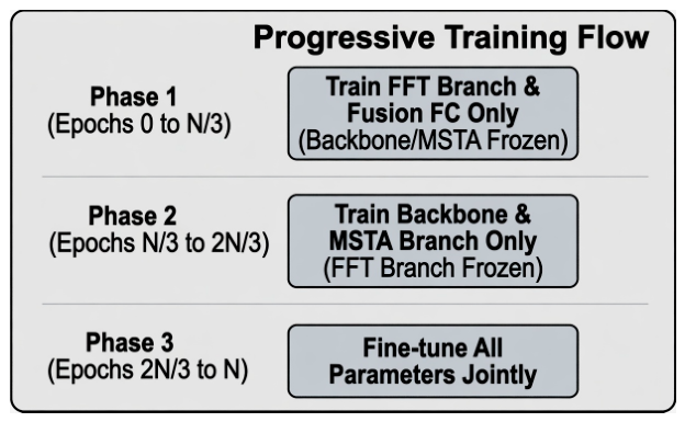
To address the challenge of training a complex dual-branch architecture where one modality might dominate the learning process, a three-phase progressive training strategy is introduced as in Figure 4.

In the initial phase, we prioritize the Global Frequency Branch. The ResNeXt-50 backbone and the Multi-Scale Transmission Attention (MSTA) module are frozen, preventing any update to the spatial weights. The network is forced to minimize visibility regression error solely through frequency-domain analysis. This phase ensures that the spectral gating mechanism and the FFT MLP become highly sensitive to the structural blurring and spectral decay caused by atmospheric haze, establishing a robust frequency-domain baseline.

During the second phase, the frequency branch is frozen, and the Spatial Transmission Branch is unfrozen. The model now utilizes its pre-trained ImageNet weights to adapt to haze-specific spatial patterns. By training the MSTA module in isolation from spectral updates, the network focuses on learning the distribution of haze and the generation of accurate transmission maps $\mathbf{T}\left(x\right)$. This prevents the spatial features from being affected by already converged frequency features, ensuring that both branches develop independent and complementary predictive power.

In the final phase, all constraints are removed. Both branches and the fusion MLP are trained jointly. This “harmonization” phase allows the network to fine-tune the interaction between spatial and frequency features, optimizing the concatenation and final regression layers. This holistic approach ensures that the final visibility estimation $V_{pred}$ benefits from a balanced synthesis of local haze density and global spectral degradation.

2.4.2. Optimization and Regularization

We employ the AdamW optimizer [28] configured with a learning rate of ${10}^{-4}$ and a weight decay of ${10}^{-4}$. AdamW is specifically chosen for its superior decoupling of weight decay, which is critical for preventing overfitting in the deep ResNeXt backbone while maintaining stable gradient updates. To manage convergence, a ReduceLROnPlateau scheduler monitors the validation loss. If the loss fails to improve for five consecutive epochs, the learning rate is decayed by a factor of 0.5. This strategy facilitates a coarse-grained search in the initial phases and fine-grained weight adjustments during the final end-to-end fine-tuning.

Table 2. The hyperparameters for our proposed VISR-CNN.

Category	Hyperparameter	VISR-CNN
Optimization	Optimizer	AdamW
	Learning Rate	$1\times {10}^{-4}$
	Weight Decay	$1\times {10}^{-4}$
Training	Total Epochs	180 (Progressive)
	Batch Size	32
	Training Strategy	3-Phase
Architecture	Backbone Architecture	FFT + ResNeXt-50
	Attention Type	Multi-Scale Transmission
Loss Function	Primary Objective	Physics-Informed (MSE + MAE + Ranking)
	Target Output	Regression
Data	Resolution	224 × 224
	Augmentation	Rotation, Color Jitter, Resize, Crop

summarizes the hyperparameters in detail for our proposed VISR-CNN.

2.4.3. Training Dataset and Equipment

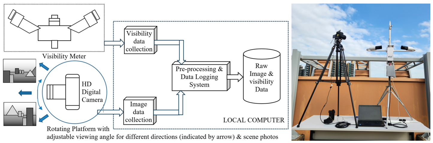
A primary challenge in visibility estimation research is the scarcity of large-scale, publicly available datasets featuring high-quality, instrument-calibrated ground truth visibility values. To resolve this and support reproducible research, we constructed the Hong Kong Chu Hai College Visibility Dataset (HKCHC-VD), which comprises 11,148 images paired with corresponding certified visibility measurements. High-resolution images (6960 × 4640 pixels) were captured using a Canon EOS 90D camera equipped with an 18 mm lens. The camera was aligned precisely with a Biral SWS-100 sensor, allowing for synchronous data acquisition via a computer interface. This sensor provides certified measurements across a range from 10 m to 75 km, with its accuracy validated against reference transmissometers. The schematic diagrams for the experimental setup are shown in Figure 5.

Data collection was performed from 8:00 to 18:00 daily for two months across diverse atmospheric conditions in Hong Kong. Images exhibiting extreme lens flare, heavy rain, or physical obstructions were subsequently removed to ensure data integrity. Reflecting real-world meteorological conditions, the dataset exhibits an inherent distribution imbalance. Specifically, a higher frequency of measurements was recorded in the range between 30 and 50 km, while the range between 0 and 10 km contains fewer samples.

Experiments were conducted on a Linux system equipped with an NVIDIA RTX 5090 GPU. Furthermore, the dataset was partitioned into a training set containing 8921 images, which represents 80% of the total data, and a testing set containing 2227 images, representing the remaining 20%. The distribution of these subsets across visibility ranges is detailed in

Table 3. HKCHC-VD, CP1 and SWH Visibility Datasets.

Dataset: HKCHC-VD	Visibility Range (km)
	0–10	10–30	30–50
No. of Training Sample Images	239	3192	5490
No. of Test Sample Images	59	797	1371
Total:	298	3989	6861
Dataset: CP1	Visibility Range (km)
	0–10	10–30	30–50
No. of Training Sample Images	386	2059	400
No. of Test Sample Images	97	515	100
Total:	483	2574	500
Dataset: SWH	Visibility Range (km)
	0–10	10–30	30–50
No. of Training Sample Images	347	2742	2710
No. of Test Sample Images	87	686	678
Total:	434	3428	3388

.

To evaluate the generalization and robustness of the VISR-CNN framework across diverse geographic and meteorological conditions, we employed two additional distinct datasets, CP1 and SWH, which were sourced from the Hong Kong Observatory (HKO). CP1 corresponds to Central Pier, and SWH corresponds to Sai Wan Ho. The images and their corresponding visibility measurements were collected between 08:00 and 18:00 daily over two months. As detailed in Table 3, CP1 consists of 3557 images, with the majority (2574) falling within the 10–30 km range, providing a rigorous test for the model’s sensitivity to subtle atmospheric changes. The SWH dataset features a balanced distribution between medium-range (10–30 km) and long-range (30–50 km) visibility, totaling 3428 medium-range and 3388 long-range samples, respectively. This dataset is particularly valuable for testing the model’s ability to discern distant structural features under clear-sky conditions.

The distribution of samples across visibility ranges (Table 3) reflects the operational and climatological reality of the collection sites. Cameras are positioned to provide mid-to-high observational ranges, leading to a higher volume of data in the 10–30 km and 30–50 km categories. By training on this natural distribution, the VISR-CNN is better prepared for real-world deployment where low-visibility events are critical but statistically less frequent.

2.5. Architectural Originality and System Summary

To summarize, the VISR-CNN framework is designed as a synergistic integration of established feature extractors and novel, physics-informed modules. To clarify the distinction between prior works and our theoretical contributions, the system components are categorized as follows:

• Spatial Backbone (Established): The use of ResNeXt-50 provides a robust baseline for high-level semantic feature extraction. While the architecture is established for standalone image feature extraction tasks, it functions here as a ‘local texture sensor’ within a dual-stream visibility framework specialized for this task.
• Frequency Branch (Enhanced): While FFT-based learning has been explored in general image processing, our implementation introduces a Global Frequency Branch specifically tuned to capture the low-pass filtering effects caused by atmospheric particles.
• Novel Spectral Gating (Original): This is a key innovation based on our practical observations that full-spectrum analysis tends to introduce atmospheric noise. The learnable masks are a unique contribution of this work.
• Multi-Scale Transmission Attention (Original): Unlike standard spatial attention, this mechanism is theoretically derived from the physics of contrast degradation and is a novel contribution of the authors.
• Monotonic Ranking Loss (Original): This represents a theoretical shift from simple regression to physics-constrained supervision, ensuring that the model strictly adheres to the physical law of light attenuation.

The validation of these components is conducted through the ablation study in Section 3.2.1, ensuring that each original contribution provides a statistically significant improvement over the established baselines.

3. Experimental Results

This section outlines the experimental objectives, evaluation strategy, and sequence of experiments used to validate the proposed visibility estimation framework. The primary goal is to quantify the prediction performance using prediction error (regression) across diverse atmospheric conditions. The experimental results comprise controlled ablation studies, comparisons with different approaches to confirm the methodology of the proposed framework.

3.1. Quantitative Comparison

To evaluate the effectiveness of the proposed VISR-CNN, we compared its performance against VisNet [10], ResNeXt-50 + ViT (spatial-threshold) [29], and three state-of-the-art Large Vision-Language Models (LVLMs) [30,31], including Qwen3-VL [32], Gemma3 [33], and Llama4 [34]. For the conventional neural network-based approaches, we adhered to the original architectural configurations and trained them using the AdamW optimizer with a learning rate of ${10}^{-4}$. To adapt the LVLMs for this visibility estimation task, we utilized a zero-shot inference framework. Images were uploaded to the models paired with a structured text prompt: ‘You are a meteorological expert. Analyze this image and estimate the atmospheric visibility distance in meters. Return only the numerical value.’

The evaluation metrics used are Mean Absolute Error (MAE) and Root Mean Squared Error (RMSE), measured in kilometers.

Table 4. Performance comparison of different methods on visibility estimation across varying ranges on HKCHC-VD, CP1 and SWH datasets.

Dataset: HKCHC-VD	Low 0–10 km		Mid 10–30 km		High 30–50 km		Overall
	MAE	RMSE	MAE	RMSE	MAE	RMSE	MAE	RMSE
VisNet [10]	2.35	4.36	1.48	2.12	1.91	2.79	1.77	2.63
ResNeXt-50 + ViT [29]	1.73	2.69	1.26	1.78	1.84	2.67	1.62	2.39
Qwen3-VL (8B) [32]	4.13	5.62	7.36	8.99	20.12	21.66	15.13	17.85
Gemma3 (12B) [33]	5.60	6.37	9.88	11.26	28.17	29.08	21.03	23.81
Llama4 (16 × 17B) [34]	4.55	5.75	12.82	15.33	23.29	25.74	19.05	22.20
VISR-CNN	1.45	1.95	1.17	1.68	1.76	2.62	1.54	2.31
Dataset: CP1	Low 0–10 km		Mid 10–30 km		High 30–50 km		Overall
	MAE	RMSE	MAE	RMSE	MAE	RMSE	MAE	RMSE
VisNet [10]	4.2	5.31	3.93	4.95	9.74	11.12	4.78	6.24
ResNeXt-50 + ViT [29]	1.47	2.26	2.87	4.03	5.64	7.00	3.07	4.399
Qwen3-VL (8B) [32]	5.00	6.08	6.86	8.54	15.59	17.70	7.83	10.09
Gemma3 (12B) [33]	5.33	5.99	5.60	7.00	20.38	21.09	7.64	10.14
Llama4 (16 × 17B) [34]	3.16	4.16	7.23	8.59	19.06	20.32	8.34	10.66
VISR-CNN	1.23	1.90	2.38	3.48	4.63	6.09	2.54	3.80
Dataset: SWH	Low 0–10 km		Mid 10–30 km		High 30–50 km		Overall
	MAE	RMSE	MAE	RMSE	MAE	RMSE	MAE	RMSE
VisNet [10]	4.14	5.20	4.52	5.67	5.53	6.90	4.97	6.25
ResNeXt-50 + ViT [29]	2.05	2.48	3.19	4.51	4.33	5.58	3.65	4.95
Qwen3-VL (8B) [32]	3.55	4.40	7.36	8.97	23.76	25.51	14.65	18.40
Gemma3 (12B) [33]	5.90	6.68	7.84	9.28	28.07	28.95	17.03	20.73
Llama4 (16 × 17B) [34]	3.04	3.61	10.47	11.49	29.77	30.57	18.87	22.22
VISR-CNN	1.00	1.49	2.27	3.58	3.81	5.24	2.91	4.36

summarizes the quantitative results across three distinct visibility ranges: Low (0–10 km), Mid (10–30 km), and High (30–50 km), using the HKCHC-VD, CP1 and SWH datasets.

3.1.1. Comparison with Specialized Models

As observed in Table 4, the proposed VISR-CNN achieves the best performance across the low, mid, and high-visibility ranges at all three distinct geographic locations (CHC, CP1, and SWH). On the primary HKCHC-VD dataset, VISR-CNN achieves an overall MAE of 1.54 km and RMSE of 2.31 km. This represents a significant improvement over the VisNet [10] and ResNeXt-50 + ViT [29], reducing the overall MAE by approximately 13% (from 1.77 km to 1.54 km) and 5% (from 1.62 to 1.54), respectively. The performance gap is most pronounced in the low visibility range between 0 and 10 km, which is the most critical scenario for safety-critical applications. In this range, VAR-CNN reduces the RMSE from 4.36 km (VisNet) and 2.69 km (ResNeXt-50 + ViT) to 1.95 km. Crucially, consistent performance gains are further validated on the CP1 and SWH datasets. Compared to ResNeXt-50 + ViT [29], VISR-CNN reduces overall MAE by approximately 21% (from 3.07 km to 2.54 km) and 20% (from 3.65 km to 2.91 km), respectively, which confirms the model’s robust generalization across diverse geographical locations. This demonstrates that the integration of the Multi-Scale Transmission Attention module effectively allows the network to focus on haze-relevant features even when visual cues are heavily degraded.

While the datasets exhibit a natural imbalance characteristic of meteorological phenomena, where the 10–30 km and 30–50 km ranges represent the majority of samples, the performance gains of VISR-CNN remain statistically robust across all categories. To evaluate the impact of this imbalance, we performed a cross-validation analysis across the HKCHC-VD, CP1, and SWH datasets. Despite the differing concentrations of samples (e.g., the number of high-visibility samples in SWH is eight times that in CP1), VISR-CNN maintained a consistent improvement margin over baseline models. The lowest MAE values of 1.45, 1.23 and 1.00 in the 0–10 km range for the HKCHC-VD, CP1 and SWH datasets, respectively, are particularly indicative of the model’s ability to generalize from limited but physically critical data points.

3.1.2. Comparison with Large Vision-Language Models (LVLMs)

The experimental results highlight a significant limitation of general-purpose generative models, such as Qwen3-VL (8B) [32], Gemma3 (12B) [33], and Llama4 (16 × 17B) [34], for precise meteorological regression tasks. As summarized in Table 4, all three LVLMs consistently exhibit high error rates across all three datasets (CHC, CP1, and SWH). Overall, MAE values are achieved ranging from 15.13 km to 21.03 km, from 7.64 km to 8.34 km, and from 14.65 km to 18.87 km on HKCHC-VD, CP1 and SWH respectively. Furthermore, the performance of LVLMs degrades catastrophically in the high visibility range between 30 and 50 km, with Gemma3 recording an MAE of 28.17 km on HKCHC-VD and with Llama4 recording an MAE of 29.77 km on SWH. This suggests that while LVLMs may recognize fog in the low range, they lack the calibrated continuous understanding required to distinguish between varying degrees of clear sky transparency. The comparison confirms that massive parameter counts do not substitute for domain-specific architectural designs, such as our Global Frequency Branch and physics-informed loss, which constrain predictions to physically plausible values.

3.1.3. Visual Analysis of Model Predictions

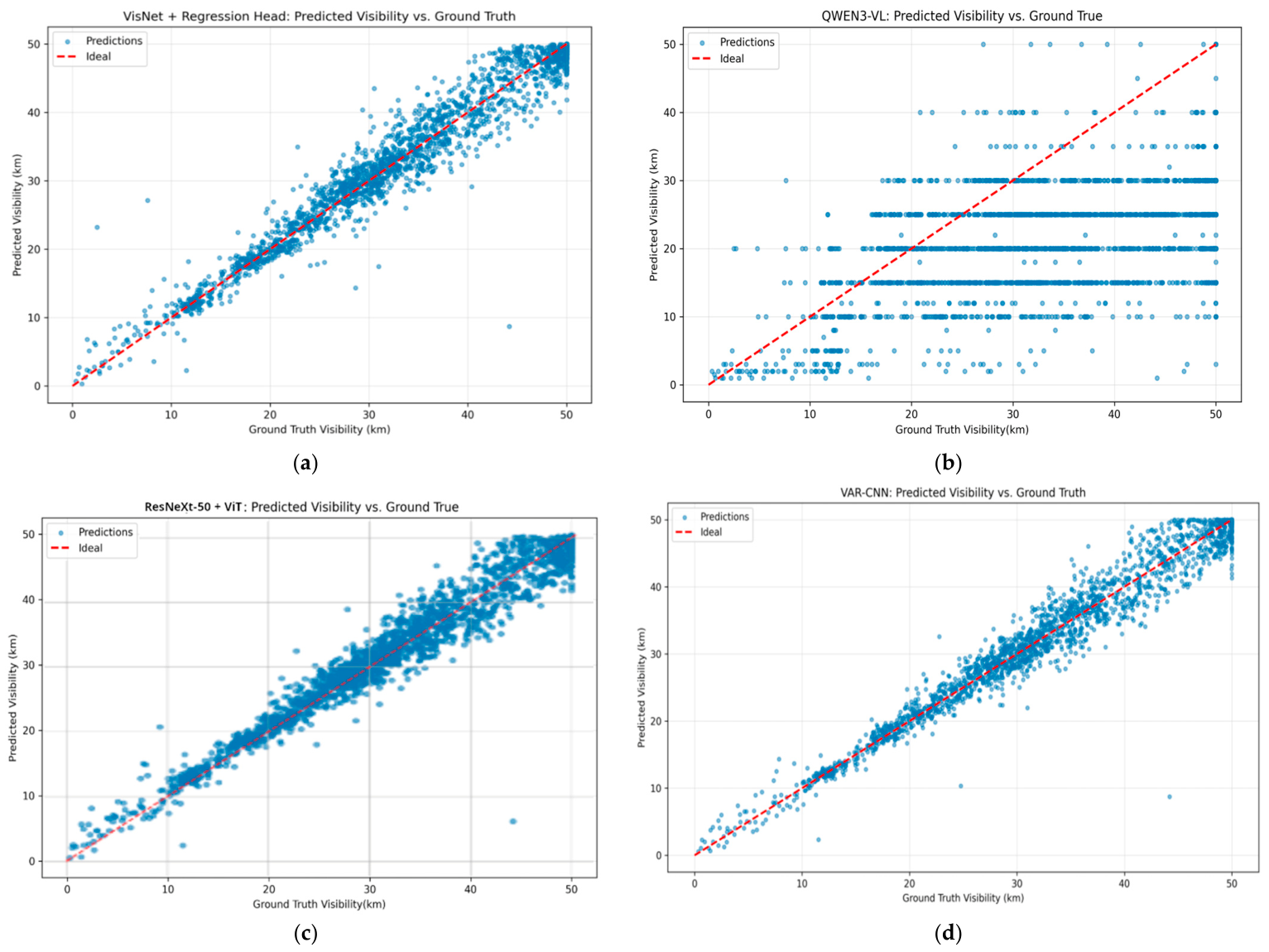
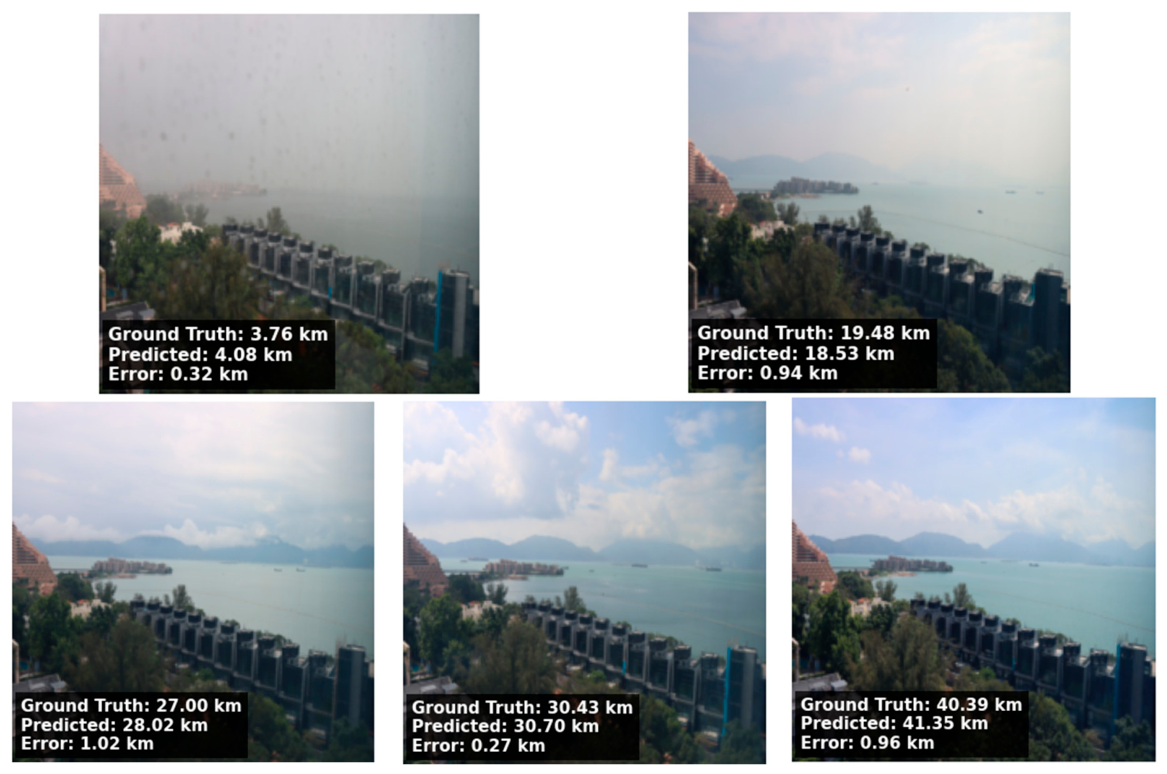
Figure 6 illustrates the relationship between ground truth and predicted visibility for different models, while Figure 7 presents qualitative examples across the full measurement spectrum. As shown in the scatter plots, VISR-CNN exhibits the highest density of points along the ideal identity line, which indicates superior regression stability. In contrast, Qwen3-VL displays a discretized striping effect, revealing that general purpose models struggle to output precise continuous values for meteorological regression. Furthermore, as shown in the scatter plots, VISR-CNN exhibits superior regression stability across the entire 0–50 km spectrum. This performance is particularly significant when contrasted with traditional edge-based algorithms such as Robert’s [5], which collapse in conditions below 400 m due to the loss of sharp gradients. Furthermore, while more recent architectures like VisNet and ResNeXt-50 + ViT show significant variance at high visibility ranges, VISR-CNN’s integration of spectral features ensures high precision in both dense fog and clear-sky scenarios.

The qualitative examples in Figure 7 further validate the robustness of the framework across diverse weather conditions. Even in dense haze where the ground truth is only 3.76 km, the model achieves a prediction of 4.08 km, which represents a minimal error of only 0.32 km. As the scene transitions to clearer atmospheric states, such as the example with a ground truth of 40.39 km, the prediction remains highly accurate at 41.35 km. This consistency confirms that the dual branch architecture effectively extracts depth cues and spectral information regardless of the baseline luminance or haze concentration.

A critical challenge noted was the scarcity of data in the range between 0 and 10 km, specifically 239 training samples compared to 3087 samples for the range between 40 and 50 km. Despite this severe imbalance, our multi-task loss function allowed the model to achieve high regression precision compared to other approaches. This demonstrates that the integrated ranking loss prevents the model from becoming biased toward the over-represented clear weather samples, ensuring reliable performance during hazardous low visibility events.

3.1.4. Visualization for the Multi-Scale Transmission Attention (MSTA)

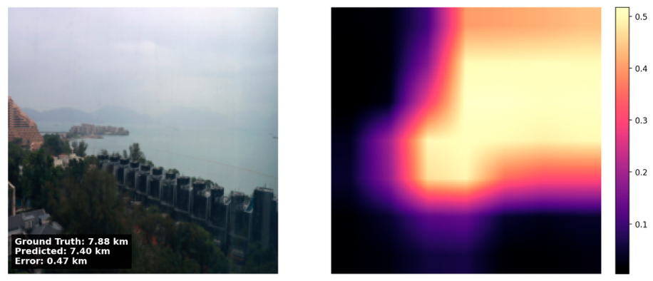
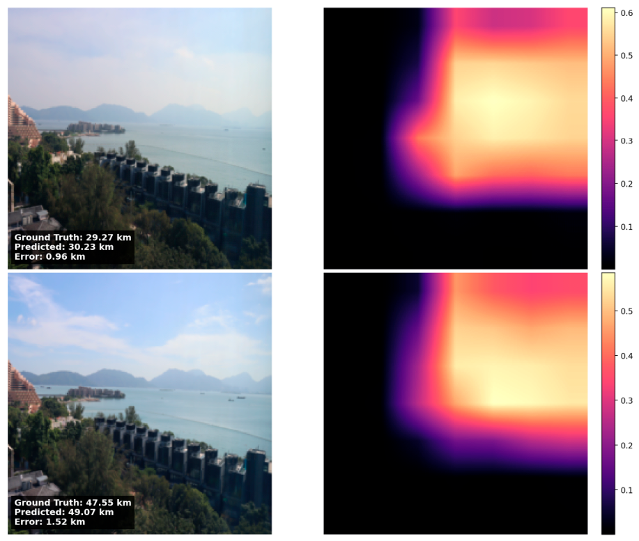
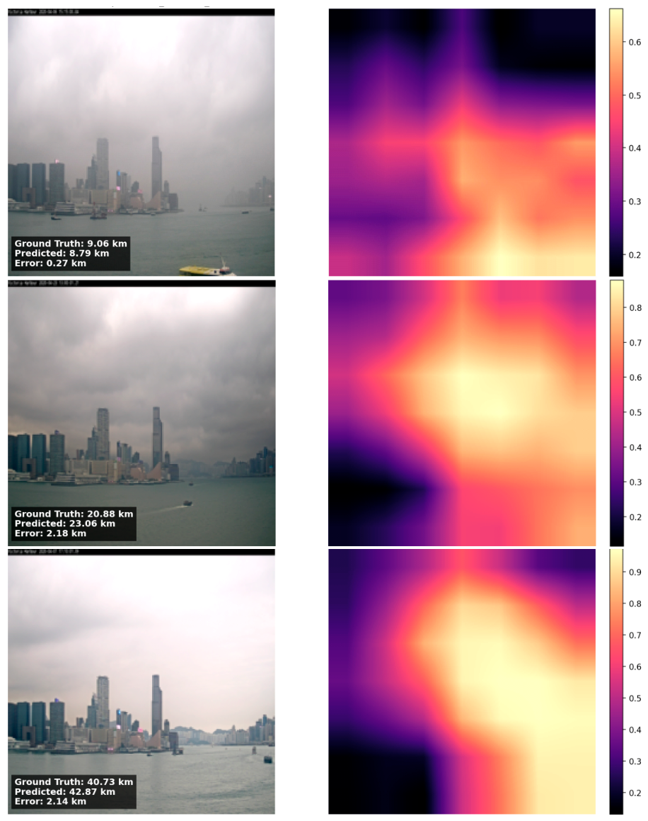
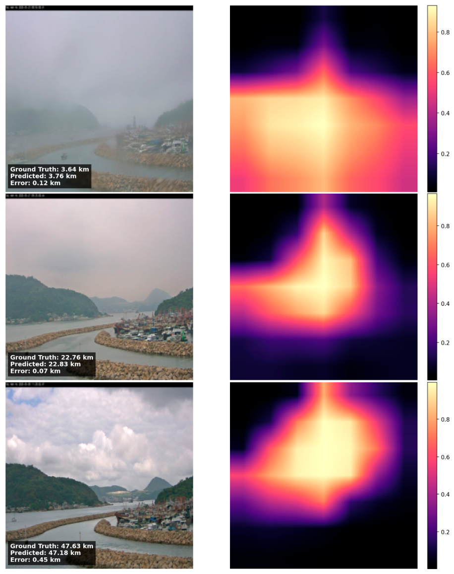
To further validate the effectiveness of the spatial attention mechanism, we visualized the transmission maps generated by the Multi-Scale Transmission Attention (MSTA) module. The heatmaps reveal a dynamic adaptation strategy aligned with the physical properties of atmospheric scattering. Figure 8, Figure 9 and Figure 10 visualize the heatmaps on the HKCHC-VD, CP1, and SWH datasets, respectively.

Under low-visibility conditions (e.g., fog or heavy haze), the learnable attention weights exhibit higher activation in the foreground and regions of higher contrast, where structural details are still perceivable. Conversely, in clear weather scenarios, the attention map shifts its priority toward the horizon line and distant landmarks. This behavior suggests that the VISR-CNN adaptively modulates its spatial focus: prioritizing proximal structural features when the extinction coefficient is high and extending its focus to farther spatial regions when the atmosphere is clear. This confirms that the MSTA mechanism effectively learns the correlation between spatial feature distribution and the physical density of atmospheric haze.

3.1.5. Visualization for the Spectral Gating (SG)

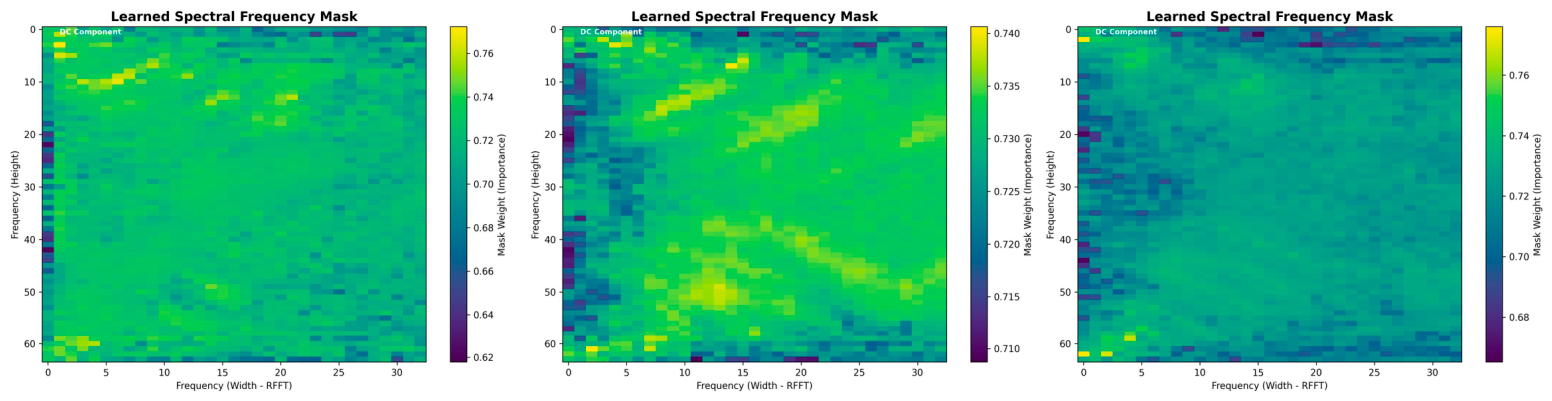
We also visualize the learnable masks that applied to the frequency components after the Real Fast Fourier Transform (RFFT) at Spectral Gating (SG) as in Figure 11.

• Priority on Low Frequencies (Top-Left Corner): In all datasets, the highest weights (bright yellow/green) are concentrated near the DC Component and low-frequency regions. This indicates that the model prioritizes global structures and large-scale intensity variations, which are the primary indicators of atmospheric haze and fog density in meteorological visibility estimation.
• Adaptive Filtering of High Frequencies: The darker regions (purple/dark blue) represent higher frequency bands that are suppressed by the gating mechanism. These frequencies typically correspond to sharp edges or transient sensor noise that could interfere with stable visibility regression.
• Consistency Across Datasets: While the specific distribution of weights varies slightly between the two datasets (reflecting site-specific environmental features), both masks consistently favor the low-to-mid frequency range. This demonstrates that the Spectral Gating mechanism successfully learns a robust, physically consistent filter for visibility-related spectral features regardless of the specific deployment location.

3.2. Ablation Study and Efficiency Analysis

In this section, we conduct a series of ablation experiments and a complexity analysis to isolate the performance gains attributed to each module of the VISR CNN framework. The goal is to verify how the Global Frequency Branch, the Multi Scale Transmission Attention (MSTA) module, and the Progressive Training Strategy collectively enhance regression accuracy while maintaining a low computational footprint. By comparing the full model against various baseline configurations, we provide a quantitative justification for the proposed dual stream design and its operational efficiency in real time applications.

3.2.1. Component Efficiency and Dual-Stream Integration

Table 5. Performance comparison of single backbone on visibility estimation on HKCHC-VD dataset.

Methods	Low 0–10 km		Mid 10–30 km		High 30–50 km		Overall
	MAE	RMSE	MAE	RMSE	MAE	RMSE	MAE	RMSE
ResNeXt-50 Single Backbone	2.24	2.96	1.45	2.06	1.83	2.83	1.71	2.59
FFT Single Backbone	3.15	5.49	2.13	3.15	2.92	3.99	2.50	3.64
VISR-CNN (without progressive)	1.51	2.29	1.22	1.84	1.81	2.69	1.59	2.41
VISR-CNN (without ranking loss)	1.51	2.28	1.18	1.69	1.82	2.71	1.58	2.38
VISR-CNN (without MSTA and SG)	1.68	2.62	1.21	1.68	1.82	2.71	1.60	2.39
VISR-CNN	1.45	1.95	1.17	1.68	1.76	2.62	1.54	2.31

provides a comprehensive breakdown of the individual contributions of each architectural component. The necessity of the proposed dual-stream framework is established through the following comparisons:

• Spatial Baseline (ResNeXt-50 Single Backbone): Achieves an overall RMSE of 2.59 km but degrades to 2.96 km in the 0–10 km range. This confirms that spatial landmarks become unreliable when obscured by dense atmospheric particles.
• Spectral Baseline (FFT Single Backbone): Exhibits the highest error (RMSE: 3.64 km). While capturing global blurring patterns, the lack of localized spatial awareness results in poor precision across all ranges.
• Fusion Baseline (VISR-CNN (without progressive)): achieves RMSE of 2.41 km, confirming that spatial and spectral features provide complementary information for stabilizing predictions.
• MSTA and SG (VISR-CNN (without MSTA and SG)): Removing MSTA and SG increases overall RMSE to 2.39 km. The full model’s 3.5% improvement proves the SG and MSTA modules function as an adaptive mechanism for frequency and spatial domains respectively, effectively isolating visibility-dependent spectral features from complex atmospheric interference.
• Physics-Informed Ranking Loss (VISR-CNN (without ranking loss)): Excluding this loss results in a sharp performance drop in the safety-critical 0–10 km range (RMSE increases from 1.95 km to 2.28 km). This validates the module’s role in enforcing monotonic physical constraints between atmospheric extinction and image contrast.
• Full VISR-CNN: Yields the optimal RMSE of 2.31 km. By isolating branch training before joint fine-tuning, the strategy prevents the high-gradient spatial branch from overwhelming frequency features, ensuring a robust multi-modal representation.

3.2.2. Impact of Progressive Training Strategy

The most critical findings emerge from the comparison between the standard and progressive training versions of the proposed architecture. The full VISR-CNN, optimized via the three-phase progressive strategy, achieves a superior overall RMSE of 2.31 km and an MAE of 1.54 km, establishing it as the most robust configuration in this study. The impact of this progressive curriculum is most pronounced in critical safety scenarios between 0 and 10 km, where the RMSE decreases from 2.29 km to 1.95 km. This 14.8% relative improvement underscores the importance of decoupled optimization in multi-modal networks.

In the non-progressive variant, the high-dimensional spatial features from the ResNeXt-50 backbone tend to dominate the gradient flow during the early stages of training, a phenomenon which often suppresses the learning of the auxiliary frequency branch. By pre-training the spectral gating mechanism in Phase 1 before introducing the spatial backbone, we ensure that the model develops a robust, independent understanding of global atmospheric degradation. This staged approach allows for a more harmonious feature fusion in the final joint fine-tuning phase, ultimately producing a system that is significantly more resilient to the extreme visual degradation characteristic of dense haze scenarios.

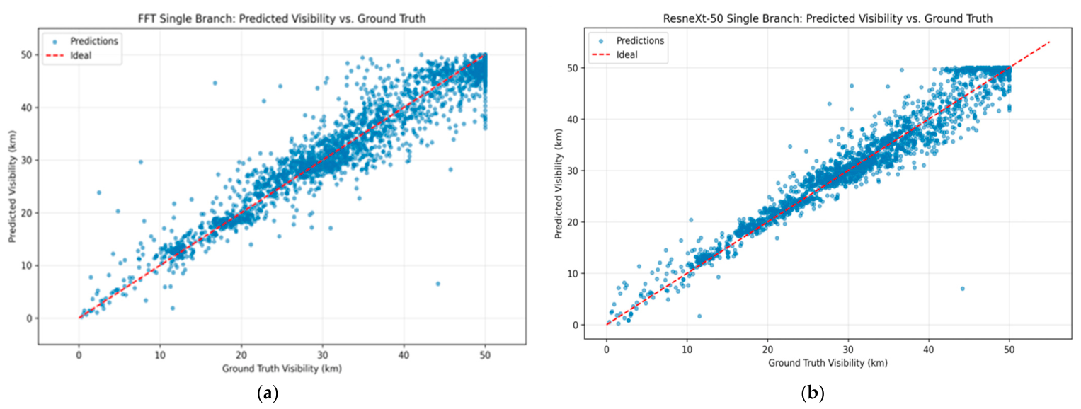
3.2.3. Visual Analysis of Single Backbone Model Predictions

It can be observed from Figure 12, which plots the ground truth against the predicted visibility for the FFT single branch and ResNeXt-50 single branch, that the dual branch architecture with progressive training outperforms the single branch approaches. These results demonstrate that the full VISR-CNN approach yields significant improvements for visibility estimation relative to standalone single branch methods. By comparing the scatter distributions, it becomes evident that while the individual backbones struggle with variance in the range between 0 and 50 km, the integrated VISR-CNN maintains a much tighter alignment with the identity line, confirming that the fusion of spatial and spectral features effectively mitigates the errors inherent in single modality estimation.

3.2.4. Analysis of Computational Complexity

The analysis of model complexity and inference speed is shown in

Table 6. Comparison of Model Complexity and Inference Speed.

Framework	Params (M)	FLOPs (G)	Latency (ms)
ResNeXt-50 Single Backbone	24.16 M	4.29	1.94
FFT Single Backbone	34.68 M	0.08	0.18
ResNeXt-50 + ViT (dual-threshold)	113.93 M	15.58	5.53
VISR-CNN	90.76 M	5.7	2.76

. By comparing the ResNeXt-50 single backbone, FFT single backbone, and ResNeXt-50 + ViT (dual threshold), we observe that the VISR-CNN architecture provides a balanced trade-off between accuracy and efficiency. Specifically, while the ResNeXt-50 + ViT model requires 113.93 million parameters and 15.58 G FLOPs, VISR-CNN achieves superior performance with only 90.76 million parameters and 5.7 G FLOPs.

This represents a significant reduction in computational overhead, as VISR-CNN is approximately 2.7 times faster in terms of latency (2.76 ms versus 5.53 ms) compared to the ResNeXt-50 + ViT (dual-threshold) model. Although the FFT single backbone is the most lightweight with a latency of 0.18 ms, its high error rates make it unsuitable for high precision tasks. Thus, the VISR-CNN architecture succeeds in delivering high accuracy while remaining efficient enough for real-time meteorological monitoring applications.

4. Discussion

The experimental results presented in this study validate the effectiveness of the VISR-CNN architecture in addressing the complexities of meteorological visibility estimation. A primary observation is the significant performance gap between our specialized dual-stream approach and general-purpose Large Vision-Language Models (LVLMs). While models such as Qwen3-VL and Llama4 possess an immense capacity for semantic reasoning, their high error rates in visibility regression suggest a fundamental limitation in mapping visual atmospheric degradation to continuous numerical values. It appears that while an LVLM can write a poem about fog, it is remarkably prone to high visibility collapse, where it fails to distinguish subtle contrast differences in clear conditions. This is likely due to a lack of domain-specific constraints. In contrast, by grounding the VISR-CNN in a physics-informed framework, we ensure that the model prioritizes structural integrity and light attenuation patterns over purely linguistic or semantic priors.

Theoretically, the success of the VISR-CNN can be attributed to its alignment with the physical properties of atmospheric light scattering. Meteorological visibility fluctuates across annual cycles, which range from uniform Spring fog to non-homogeneous summer haze. Each presenting distinct optical signature. Our Multi-Scale Transmission Attention (MSTA) module addresses this by utilizing dilated convolutions to capture haze at multiple receptive fields. This design is theoretically consistent with the need to approximate the transmission map $T\left(x\right)$ across varying aerosol optical depths, allowing the model to simultaneously analyze local foreground textures and global airlight intensity.

Furthermore, the synergy between the Global Frequency Branch and the spatial backbone highlights the importance of dual domain analysis. From a theoretical perspective, atmospheric haze acts as a spatial low-pass filter that suppresses high-frequency edge information. In scenarios of extreme haze (0–10 km range), where spatial landmarks are nearly invisible to the human eye, the frequency domain provides a stable spectral signature of this filtering effect. By transforming the image into the spectral domain via RFFT2D, the model can adaptively identify the specific “spectral footprint” of seasonal weather profiles that a purely spatial model might overlook. Table 5 empirically supports these theories; specifically, in the low-visibility range (0–10 km), the removal of the MSTA and Spectral Gating (SG) modules caused the MAE and RMSE to degrade to 1.68 and 2.62, respectively, representing a significant loss in precision compared to the full architecture.

Our Progressive Training Strategy was instrumental in managing this synergy. By preventing the high dimensional spatial branch from dominating the gradient flow in the early epochs, the model was forced to develop a robust spectral sensitivity. This ensures the network adheres to the physical principle of monotonic degradation, where increased atmospheric particulate matter must mathematically correspond to a decrease in visibility. Results from Table 5 indicate that without progressive training, performance across all ranges suffered: MAE in the low-visibility range (0–10 km) degraded by approximately 4%, the mid-visibility range (10–30 km) by 4.1%, and the high-visibility range (30–50 km) by 2.8%. This balanced optimization is precisely what enables VISR-CNN to maintain high accuracy even when visual landmarks are largely absent, providing a more rigorous foundation for the regression task than standard single-stage training.

5. Conclusions

In this paper, we introduced the Visibility-Aware Refined CNN (VISR-CNN), a specialized framework that integrates spatial and spectral features for high-precision meteorological visibility estimation. By combining a ResNeXt-50 backbone with a dedicated Global Frequency Branch and a Multi-Scale Transmission Attention (MSTA) module, we addressed the limitations of traditional purely spatial CNNs. Our approach was further fortified by a Progressive Training Strategy and a Physics-Informed Ranking Loss, ensuring that the model captures both the absolute numerical distance and the relative monotonic degradation of visibility.

Experimental evaluations on the HKCHC-VD dataset demonstrate that VISR-CNN sets a new benchmark in the field, achieving an overall MAE of 1.54 km and an RMSE of 2.31 km. Crucially, the model’s robust generalization is validated by extensive testing on the CP1 and SWH datasets, where it consistently outperformed the hybrid ResNeXt-50 + ViT model, reducing overall MAE by 21% and 20%, respectively. The model’s performance in the safety-critical range from 0 to 10 km, where it achieved RMSE reductions of over 55%, 64%, and 71% for the HKCHC-VD, CP1, and SWH datasets compared with VisNet, highlights its potential for integration into autonomous driving and aviation monitoring systems. Moreover, our comparison with state-of-the-art LVLMs underscores the continued necessity of specialized, domain-aware architectures for scientific regression tasks.

Future research will focus on three primary directions to extend the utility and scalability of the VISR-CNN framework. First, to enhance operational robustness, we aim to transition from single-frame estimation to video-based sequence analysis for improved temporal stability. This will be coupled with the integration of multi-modal data, such as infrared or depth information, to maintain accuracy under extreme low-light or nighttime conditions. Second, to address data scalability, we will explore cross-domain adaptation via generative AI, specifically, using diffusion models or GANs to synthesize high-fidelity visibility-degraded datasets for geographic regions where ground-truth sensors are scarce. Finally, to achieve intelligence expansion, we plan to integrate VISR-CNN with Vision-Language Models (VLMs) to enable descriptive visibility analysis, providing natural language explanations of atmospheric conditions alongside numerical estimates. These advancements, paired with optimization for edge-computing deployment, will facilitate real-time, localized visibility monitoring for smart cities.

References

1. He, K.; Sun, J.; Tang, X. Single image haze removal using dark channel prior. IEEE Trans. Pattern Anal. Mach. Intell. 2011, 33, 2341–2353. [Google Scholar] [PubMed]
2. Nayar, S.K.; Narasimhan, S.G. Vision in bad weather. In Proceedings of the Seventh IEEE International Conference on Computer Vision, Corfu, Greece, 20–27 September 1999; IEEE: Piscataway, NJ, USA, 1999; pp. 820–827. [Google Scholar]
3. Narasimhan, S.G.; Nayar, S.K. Vision and the atmosphere. Int. J. Comput. Vis. 2002, 48, 233–254. [Google Scholar] [CrossRef]
4. World Meteorological Organization. Guide to Meteorological Instruments and Methods of Observation, 2018th ed.; WMO-No. 8; WMO: Geneva, Switzerland, 2018. [Google Scholar]
5. Robert, G.H.; Michael, P.M. An Automated Visibility Detection Algorithm Utilizing Camera Imagery. In Proceedings of the 23rd Conference on IIPS, San Antonio, TX, USA, 15 January 2007. [Google Scholar]
6. Babari, R.; Hautiere, N.; Dumont, E.; Bredif, R.; Paparoditis, N. A Model-Driven Approach to Estimate Atmospheric Visibility with Ordinary Cameras. Atmos. Environ. 2011, 45, 5316–5324. [Google Scholar]
7. Lo, W.L.; Zhu, M.; Fu, H. Meteorological Visibility Estimation Using Multi-Support Vector Regression Method. J. Adv. Inf. Technol. 2020, 11, 40–47. [Google Scholar]
8. Yan, Q.; Sun, T.; Zhang, J.; Xun, L. Visibility estimation based on weakly supervised learning under discrete label distribution. Sensors 2023, 23, 9390. [Google Scholar] [CrossRef] [PubMed]
9. Cai, B.; Xu, X.; Jia, K.; Qing, C.; Tao, D. DehazeNet: An End-to-End System for Single Image Haze Removal. IEEE Trans. Image Process. 2016, 25, 5187–5198. [Google Scholar] [CrossRef] [PubMed]
10. Palvanov, A.; Cho, Y.I. VisNet: Deep Convolutional Neural Networks for Forecasting Atmospheric Visibility. Sensors 2019, 19, 1343. [Google Scholar] [CrossRef] [PubMed]
11. Pan, H.; Xue, J.; Huang, M.; Lei, X. Air Visibility Prediction Based on Multiple Models. In Proceedings of the IEEE CYBER, Tianjin, China, 19–23 July 2018; pp. 1421–1426. [Google Scholar]
12. Jin, Z.; Qiu, K.; Zhang, M. Investigation of Visibility Estimation Based on BP Neural Network. J. Atmos. Environ. Opt. 2021, 16, 415–423. [Google Scholar]
13. Narksri, P.; Darweesh, H.; Takeuchi, E.; Ninomiya, Y.; Takeda, K. Visibility Estimation in Complex, Real-World Driving Environments Using High Definition Maps. In Proceedings of the IEEE ITSC, Indianapolis, IN, USA, 19–22 September 2021; pp. 2847–2854. [Google Scholar]
14. You, J.; Jia, S.; Pei, X.; Yao, D. DMRVisNet: Deep Multihead Regression Network for Pixel-Wise Visibility Estimation Under Foggy Weather. IEEE Trans. Intell. Transp. Syst. 2022, 23, 22354–22366. [Google Scholar] [CrossRef]
15. Lo, W.L.; Wong, K.W.; Hsung, R.T.C.; Chung, H.S.H.; Fu, H. Meteorological Visibility Estimation Using Landmark Object Extraction and the ANN Method. Sensors 2025, 25, 951. [Google Scholar] [CrossRef] [PubMed]
16. He, K.; Zhang, X.; Ren, S.; Sun, J. Deep Residual Learning for Image Recognition. In Proceedings of the IEEE Conference on Computer Vision and Pattern Recognition (CVPR), Las Vegas, NV, USA, 27–30 June 2016; pp. 770–778. [Google Scholar]
17. Xie, S.; Girshick, R.; Dollár, P.; Tu, Z.; He, K. Aggregated Residual Transformations for Deep Neural Networks. In Proceedings of the IEEE Conference on Computer Vision and Pattern Recognition (CVPR), Honolulu, HI, USA, 21–26 July 2017; pp. 1492–1500. [Google Scholar]
18. Moorthy, A.K.; Bovik, A.C. Blind image quality assessment: A natural scene statistics approach in the DCT domain. IEEE Trans. Image Process. 2011, 20, 3339–3352. [Google Scholar] [CrossRef] [PubMed]
19. Xu, K.; Stevens, M.; Barsky, B.A. Learning in the Frequency Domain. In Proceedings of the IEEE/CVF Conference on Computer Vision and Pattern Recognition (CVPR), Seattle, WA, USA, 14–19 June 2020; pp. 1740–1749. [Google Scholar]
20. Mittal, A.; Soundararajan, R.; Bovik, A.C. No-reference image quality assessment in the spatial domain. IEEE Trans. Image Process. 2012, 21, 4695–4708. [Google Scholar] [CrossRef] [PubMed]
21. Lo, W.L.; Wong, K.W.; Hsung, R.T.C.; Chung, H.S.H.; Fu, H.; Zhu, T.Y.; Tsang, H.S.H.; Pong, K.H. Meteorological Visibility Estimation Through Multi-Modal Feature Fusion with Convolutional and Frequency Domain Representations. In Proceedings of the International Conference on Computer and Communications (ICCC), Chengdu, China, 12–15 December 2025. [Google Scholar]
22. Xie, L.; Chiu, A.; Newsam, S. Estimating Atmospheric Visibility Using General-Purpose Cameras. In Advances in Visual Computing, Proceedings of the 4th International Symposium, ISVC 2008, Las Vegas, NV, USA, 1–3 December 2008; Bebis, G., Boyle, R., Parvin, B., Koracin, D., Remagnino, P., Nefian, A., Gantz, L.I., Eds.; Springer: Berlin/Heidelberg, Germany, 2008; Volume 5359, pp. 356–367. [Google Scholar]
23. Chen, L.C.; Papandreou, G.; Schroff, F.; Adam, H. Rethinking Atrous Convolution for Semantic Image Segmentation. arXiv 2017, arXiv:1706.05587. [Google Scholar] [CrossRef]
24. Chen, L.C.; Zhu, Y.; Papandreou, G.; Schroff, F.; Adam, H. Encoder-Decoder with Atrous Separable Convolution for Semantic Image Segmentation. In Proceedings of the European Conference on Computer Vision (ECCV), Munich, Germany, 8–14 September 2018; pp. 801–818. [Google Scholar]
25. Simonyan, K.; Zisserman, A. Very Deep Convolutional Networks for Large-Scale Image Recognition. In Proceedings of the International Conference on Learning Representations (ICLR), San Diego, CA, USA, 7–9 May 2015. [Google Scholar]
26. Frigo, M.; Johnson, S.G. The design and implementation of FFTW3. Proc. IEEE 2005, 93, 216–231. [Google Scholar] [CrossRef]
27. Nair, V.; Hinton, G.E. Rectified Linear Units Improve Restricted Boltzmann Machines. In Proceedings of the 27th International Conference on Machine Learning (ICML), Haifa, Israel, 21–24 June 2010; pp. 807–814. [Google Scholar]
28. Loshchilov, I.; Hutter, F. Decoupled Weight Decay Regularization. In Proceedings of the International Conference on Learning Representations (ICLR), New Orleans, LA, USA, 6–9 May 2019. [Google Scholar]
29. Lo, W.L.; Wong, K.W.; Hsung, R.T.C.; Chung, H.S.H.; Fu, H.; Tsang, H.S.H.; Zhu, T.Y. A Range-Aware Attention Framework for Meteorological Visibility Estimation. Sensors 2026, 26, 1893. [Google Scholar] [CrossRef] [PubMed]
30. Rahman, A. A Systematic Review of Vision Language Models: Comprehensive Analysis of Architectures, Applications, Datasets and Challenges Towards Robust Multimodal Intelligence. Array 2026, 30, 100739. [Google Scholar] [CrossRef]
31. Zhang, C.; Wan, F.; Wei, P.; Xu, K.; Guo, L.; Jiao, J.; Ye, Q. Vision-Language Models for Vision Tasks: A Survey. IEEE Trans. Pattern Anal. Mach. Intell. 2024, 46, 1234–1256. [Google Scholar] [CrossRef] [PubMed]
32. Bai, S.; Cai, Y.; Chen, R.; Chen, K.; Chen, X.-H.; Cheng, Z.; Deng, L.; Ding, W.; Fang, R.; Gao, C.; et al. Qwen3-VL Technical Report. arXiv 2025, arXiv:2511.21631. [Google Scholar] [CrossRef]
33. Gemma Team. Gemma 3 Technical Report. arXiv 2025, arXiv:2503.19786. [Google Scholar] [CrossRef]
34. Meta, A.I. The Llama 4 Herd: Architecture, Training, Evaluation, and Deployment Notes. arXiv 2026, arXiv:2601.11659. [Google Scholar] [CrossRef]
Figure 1. Progressive Training Architecture for Visibility Estimation.
Algorithms 19 00434 g001
Figure 2. Multi-Scale Transmission Attention (MSTA) Module.
Algorithms 19 00434 g002
Figure 3. Real FFT and gating processes.
Algorithms 19 00434 g003
Figure 4. Progressive Training Strategy for Visibility Estimation.
Algorithms 19 00434 g004
Figure 5. Schematic diagram and illustration of experimental setup.
Algorithms 19 00434 g005
Figure 6. Ground Truth vs. Predicted Visibility. (a) VisNet, (b) Qwen3-VL, (c) ResNeXt-50 + ViT (spatial-threshold), and (d) VISR-CNN.
Algorithms 19 00434 g006
Figure 7. Examples of predicted visibility values against ground truth.
Algorithms 19 00434 g007
Figure 8. Visualization of the MSTA mechanism on HKCHC-VD dataset. (Left: Input image. Right: Corresponding heatmap visualization of the transmission map).
Algorithms 19 00434 g008aAlgorithms 19 00434 g008b
Figure 9. Visualization of the MSTA mechanism on CP1 dataset. (Left: Input image. Right: Corresponding heatmap visualization of the transmission map).
Algorithms 19 00434 g009
Figure 10. Visualization of the MSTA mechanism on SWH dataset. (Left: Input image. Right: Corresponding heatmap visualization of the transmission map).
Algorithms 19 00434 g010
Figure 11. Visualization of the learnable masks at Spectral Gating on HKCHC-VD (Left), CP1 (Middle), and SWH (Right) dataset.
Algorithms 19 00434 g011
Figure 12. Ground Truth vs. Predicted Visibility. (a) FFT single branch, and (b) CNN single branch.
Algorithms 19 00434 g012