A Clustering Approach for Rare Variant Classification by Effect Direction and Magnitude

Abstract

Several gene-based tests, such as the sequence kernel association test, have been developed to assess associations between rare single nucleotide variants (SNVs) and disease traits. However, these aggregate methods do not distinguish potentially causal variants from null variants within associated regions. To address this limitation, we propose gvClust, a clustering approach that classifies rare variants into null and signal groups using a Gaussian mixture model applied to variant-level summary statistics from multiple-variant models. Signal variants are further partitioned into risk and protective subgroups according to their effect direction and magnitude. We evaluated gvClust in simulation studies using the adjusted Rand index (ARI), mean squared error (MSE), and accuracy of cluster number selection under different sample sizes, effect configurations, outcome types, and linkage disequilibrium (LD) structures. In simulations, gvClust showed improved performance with increasing sample size, achieved high accuracy in determining the number of clusters for continuous traits at large sample sizes, and outperformed both k-means clustering and initialization-only clustering. We then applied gvClust to rare variants in six genes associated with blood pressure traits from a large genome-wide association study and meta-analysis. In the real-data application, gvClust identified distinct null, risk, and protective clusters. These results suggest that gvClust provides a practical framework for classifying rare variants within associated regions and may help improve the biological interpretation of rare variant signals.

1. Introduction

During the last decade, genome-wide association studies (GWASs) have identified hundreds of thousands of common genetic variants (minor allele frequency ≥ 5%) associated with numerous complex diseases and quantitative traits [1]. In addition, low-frequency variants (1% ≤ MAF < 5%) and rare variants (MAF < 1%) have been detected increasingly with the advent of next-generation sequencing technologies. Low-frequency variants and rare variants are substantial sources of unexplained heritability of various phenotypes [2].

Several gene-based tests, such as the burden test [3] and the sequence kernel association test (SKAT) [4], have been developed for association testing of aggregate effects of rare single nucleotide variants (SNVs) with disease traits within a gene or region (deemed as “signal regions” in this manuscript). It has been shown that no gene-based test is always the most powerful. The burden test performs better than SKAT when most rare variants in a region are trait-associated and have the same effect direction. Otherwise, SKAT has more power than the burden test [4]. Hence, omnibus tests, such as SKAT-O [5] and the aggregated Cauchy association test (ACAT-O) [6], are proposed to search for an optimal combination of the burden test and SKAT to provide robust summary statistics. More recent work has further expanded rare variant analysis through annotation-informed association testing, joint modeling of multiple burden masks, category-wide analysis of rare noncoding variants, scalable meta-analysis across large sequencing studies, and summary-statistic frameworks for detecting allelic series [7,8,9,10,11]. However, these methods remain focused primarily on association detection, signal aggregation, or variant prioritization at the gene or region level. Direct methods for partitioning rare variants within a trait-associated region into null, risk, and protective groups based on estimated effect direction and magnitude remain limited.

To address the knowledge gap, we propose a novel clustering approach to classify rare variants into null (i.e., those that do not contribute to the trait of interest) and signal (i.e., those that are associated with the trait) variant groups. This classification uses a Gaussian mixture model (GMM) framework applied to summary statistics from gene-based tests, which aggregate the effects of rare variants within genes [12,13]. For a given signal region associated with a disease trait, we fit multiple-variant models to obtain association statistics between phenotypes and rare variants within the region. We simulate genomic regions with independent rare variants and variants in linkage disequilibrium (LD). We evaluate the performance of the proposed method by a comprehensive simulation study with several metrics, including the adjusted Rand index (ARI), mean square error (MSE), and accuracy of the number of clusters specification. We also compare the performance of our clustering algorithm with k-means, a widely used traditional clustering method, by a comprehensive simulation study designed to evaluate clustering accuracy under multiple scenarios. We then apply our method to identify risk and protective rare variants in six genes that are significantly associated with blood pressure (BP) traits in a recent large GWAS and meta-analysis [14]. Identifying risk and protective rare variant clusters is important for understanding the biological mechanisms between rare variants and disease traits, as well as for discovering drug targets and designing gene therapies.

2. Methods

Throughout this manuscript, a symbol with a hat denotes an estimate obtained from the observed data, whereas the same symbol without a hat denotes the corresponding underlying population parameter.

2.1. Association Testing of Rare Variants

To identify gene regions harboring rare variant signals, we first performed gene-based association testing using established methods, including burden tests, SKAT, and ACAT-O [3,4,5]. These approaches aggregate rare variant effects within a genomic region to assess overall association with the phenotype. Regions demonstrating significant association were then selected for downstream clustering analysis. For each significant region, variant-level summary statistics, including estimated effect sizes and standard errors obtained from multiple-variant models, were used as input for the proposed clustering framework. Detailed descriptions of the association testing procedures are provided in the Supplementary Materials.

2.2. Multiple-Variant Model to Obtain Variant-Level Summary Statistics

If a gene region shows statistical significance with a disease trait ($p_{ACAT-O}\le \alpha$), we perform multiple-variant analysis for all rare variants within the region to account for potential LD between the rare variants. By adjusting for covariates, the multiple-variant model is given by

$$g\left({\mu }_i\right)={\alpha }_0+X_i^T\alpha +{\displaystyle {\sum }_j^J}{G}_{ij}{\beta }_j$$

(1)

where $g(.)$ is the identity function for a continuous trait and the logistic function for a binary trait. $X_i^T$ is a row vector of covariates of the i-th individual, $G_{ij}$ is the genotype of this individual at the j-th locus within the target gene region, ${\alpha }_0$ is the intercept, $\alpha$ is a vector of fixed effects of covariates, and ${\beta }_j$ (beta coefficient) is the genetic effect of the j-th genetic variant. $\widehat{{\beta }_j}$ is an estimate of ${\beta }_j$. The estimated beta coefficient $\widehat{{\beta }_j}$, its standard error $SE\left(\widehat{{\beta }_j}\right),$ and the corresponding p-value $p_j$ of the j-th rare variant are obtained from the multiple-variant model. The estimated beta coefficients and standard error statistics are used for the subsequent clustering analysis.

2.3. Gaussian Mixture Model

We adopt a Gaussian mixture model (GMM) framework for variant clustering because it provides a principled probabilistic approach to modeling heterogeneity in genetic effect sizes. In the context of rare variant analysis, variants within a genomic region may exhibit distinct effect patterns, including null, risk, and protective effects. A mixture model flexibly captures this structure by representing the observed effect estimates as arising from multiple latent subgroups. In addition, GMM allows incorporation of variant-specific uncertainty through standard errors, enabling more accurate clustering compared to distance-based methods.

The Gaussian mixture model assumes data is generated from a mixture of Gaussian (normal) distributions. We assume that each beta coefficient from a multiple-variant model has its own variance, which is estimated by $\widehat{{\sigma }_j}=SE\left(\widehat{{\beta }_j}\right)$. Hence, we do not estimate the variance of the estimated beta coefficients in our clustering algorithm. We also assume that each beta coefficient can be classified into two types of clusters: a null cluster and K signal clusters. Therefore, the total number of clusters is K* = K + 1. A null cluster includes all non-causal rare variants in a gene region. Within each of the K signal clusters, the causal variants have a similar effect on the trait. With a null cluster and K signal clusters, each estimated beta coefficient $\widehat{{\beta }_j}$ from Equation (1) follows one of the normal distributions of $N\left({\mu }_0=0,{\widehat{{\sigma }_j}}^2\right),N\left({\mu }_1,{\widehat{{\sigma }_j}}^2\right),\dots ,N\left({\mu }_K,{\widehat{{\sigma }_j}}^2\right)$, where ${\mu }_k$ is the true mean of beta estimates for rare variants classified in the same cluster. ${\widehat{{\sigma }_j}}^2$ is the estimated variance of the j-th beta coefficient from the multiple-variant model, ${\mu }_0=0$ is the mean of the null cluster. For each ${\beta }_j$, we introduce a hidden (unobserved) class label variable $D_j$, which follows a categorical distribution (that is, the generalized Bernoulli distribution). The class label variable $D_j$ indicates the component (cluster) that $\widehat{{\beta }_j}$ belongs to, that is,

$$p\left(\widehat{{\beta }_j}\left|D_j=k,{\mu }_k\right.\right)={\displaystyle \frac{1}{{\widehat{{\sigma }_j}}^2\sqrt{2\pi }}}{e}^{-{\displaystyle \frac{1}{2}}{({\displaystyle \frac{\widehat{{\beta }_j}-{\mu }_k}{\widehat{{\sigma }_j}}})}^2}$$

(2)

where $p\left(D_j=k\right)={\phi }_k$, $0\le {\phi }_k\le 1$, and ${\displaystyle {\sum }_{k=0}^K}{\phi }_k=1$.

${\phi }_k$ is the proportion of component k in the mixture distributions. The density function of each data point $\widehat{{\beta }_j}$ is given by

$$p\left(\widehat{{\beta }_j}|\mathit{\mu },\mathit{\phi }\right)={\displaystyle {\sum }_{k=1}^K}p\left(\widehat{{\beta }_j}\left|D_j=k\right.,{\mu }_k\right){\phi }_k$$

(3)

where $\mathit{\mu }=\left\{{\mu }_0,\dots ,{\mu }_K\right\}$ and $\mathit{\phi }=\left\{{\phi }_0,\dots ,{\phi }_K\right\}$. The log-likelihood function of all beta coefficients $\widehat{\mathit{\beta }}=\left\{\widehat{{\beta }_1},\dots ,\widehat{{\beta }_J}\right\}$ is given by

$$l\left(\mathit{\mu },\mathit{\phi }|\mathit{X}\right)=log\prod _{j=1}^n\sum _{k=1}^{K}p\left(\widehat{{\beta }_j}\left|D_j=k\right.\right){\phi }_k$$

$$={\sum }_{j=1}^{n}log{\sum }_{k=1}^{K}p\left(\widehat{{\beta }_j}\left|D_j=k\right.\right){\phi }_k$$

(4)

Because there is no closed-form solution for the maximum likelihood estimators (MLEs) of the parameters, the expectation–maximization (EM) algorithm is employed to find a numeric solution. The EM algorithm is an iterative method that is described in detail in the next section.

2.4. Parameter Estimation by Expectation–Maximization (EM) Algorithm

Given a fixed number of signal clusters K, we employ the EM algorithm to estimate the 2K parameters $\left\{({\mu }_k,{\phi }_k)|k=1,\dots ,K\right\}$. Because ${\phi }_k$ estimates sum to 1, that is, ${\displaystyle {\sum }_{k=0}^K}{\phi }_k=1$, ${\phi }_0$ can be estimated automatically. Therefore, there are a total of 2K parameters to be estimated by the EM algorithm. The algorithm undergoes four steps: (1) an initialization step to set the initial values of the parameters; (2) an expectation step that computes the expected value of the log-likelihood; (3) a maximization step to update the parameters by maximizing the expectation of the log-likelihood; and (4) the determination of the number of clusters K* by the minimum BIC, with 2 ≤ K* ≤ 7. We set the maximum number of clusters to 7 because we aim to classify the rare variants into three categories: null, risk, and protective. Each of the positive and negative categories can have three sub-categories: mild, moderate, and strong effect sizes. Additionally, since there are 60 rare variants in the simulation study, 7 is a reasonable maximum number of clusters. However, users applying this method can adjust the maximum number of clusters based on the variants they are studying.

2.4.1. Initialization

The EM algorithm may converge to a local optimum, and the chance of converging to a global optimum (MLE) depends essentially on the initial values of the parameters [15]. To minimize the effect of initialization, we set initial values by a crude estimation of the proportion of non-causal variants ${\phi }_0$, using a variable threshold approach. Suppose the p-values of multiple-variant models of all the rare variants within a region are $S=\left\{p_j,j=1\dots J\right\}$. We define an absolute value of the standardized beta coefficient (Z-score) as $\left|Z_j\right|={\displaystyle \frac{\left|\widehat{{\beta }_j}\right|}{SE\left(\widehat{{\beta }_j}\right)}},j=1,\dots ,J$. For each p-value, we use a variable threshold approach, that is, if $p_l$ is used as the threshold, here $p_l\in S$. We meta-analyze the $\left|Z_j\right|,$ whose corresponding p-value is $p_j\le p_l$, by the weighted sum of the Z-scores method: ${\Omega }_l={\displaystyle \frac{{\sum }_{j:p_j\le p_l}{a}_j\left|Z_j\right|}{\sqrt{{\sum }_{j:p_j\le p_l}{a}_j^2}}}$, where $a_j$ is a pre-specified weight for the j-th absolute value of the standardized beta.

Different weighting schemes can be used. We select two weighting schemes: equal weight ($a_j=1$) and weight as the inverse of the estimated standard error ($a_j={\displaystyle \frac{1}{SE\left(\widehat{{\beta }_j}\right)}},$) to assess the sensitivity of the initialization to alternative specifications. Given a specified weighting scheme, we define an optimal threshold as $p_O^{*}=\underset{p_l}{\mathrm{arg\; max}}{\Omega }_l$. Then, we define a rare variant as a preliminary signal variant if the corresponding p-value is $p_j\le p_O^{*}$; otherwise, the variant is defined as a preliminary non-signal variant. The initial value of ${\phi }_0$ can be calculated by ${\widehat{{\phi }_0}}^{\left(0\right)}=1-{\displaystyle \frac{{\sum }_j{I}_{\{p_j\le p_O^{*}\}}}{\left|S\right|}}$. $\left|S\right|$ is the number of p-values in the set. The preliminary signal variants are then clustered by K-means analysis. The remaining mixing proportion parameters $\left\{{\widehat{{\phi }_1}}^{\left(0\right)},\dots ,{\widehat{{\phi }_K}}^{\left(0\right)}\right\}$ are calculated as $1-{\widehat{{\phi }_0}}^{\left(0\right)}$, multiplied by the proportion of variants in the K signal clusters from the K-means clustering [16,17]. The initial values of the means of the signal clusters $\left\{{\widehat{{\mu }_1}}^{\left(0\right)},\dots ,{\widehat{{\mu }_K}}^{\left(0\right)}\right\}$ are set as the cluster means from the K-means analysis.

We add a constraint that the preliminary signal variants with opposite effect directions cannot be assigned to the same cluster by the K-means method. That is, the variants with positive beta coefficients and negative ones are split into two separate clusters by the K-means method. Specifically, $K=K_{+}+K_{-}$, where $K_{+}$ and $K_{-}$ are defined as the number of clusters for the variants with positive and negative beta coefficients, respectively. Then, we run K − 1 combinations ($\left(K_{+}=1,K_{-}=K-1\right),\dots ,\left(K_{+}=K-1,K_{-}=1\right)$) of the K-means analysis. The optimal cluster partition is identified by minimizing the within-cluster sum of squares (WCSS) across the K − 1 combinations:

$$\underset{S^{+},S^{-},K_{+}}{\mathrm{arg\; min}}(\sum _{k_{+}=1}^{K_{+}}\sum _{\beta \in S_{k_{+}}}{‖\beta -{\mathit{c}}_{\mathit{i}}‖}^2+\sum _{k_{-}=1}^{K-K_{+}}\sum _{\beta \in S_{k_{-}}}{‖\beta -{\mathit{c}}_{\mathit{i}}‖}^2)$$

where $S^{+}=\left\{S_1^{+},\dots ,S_{K_{+}}^{+}\right\}$ is a partition of the variants with a positive effect direction, and $S^{-}=\left\{S_1^{-},\dots ,S_{K_{-}}^{-}\right\}$ is a partition of the variants with a negative effect direction.

2.4.2. Expectation Step

Because the EM algorithm is an iterative method, we designate ${\widehat{\mathit{\mu }}}^{\left(\mathit{i}\right)}$ and ${\widehat{\mathit{\phi }}}^{\left(\mathit{i}\right)}$ as the values of $\widehat{\mathit{\mu }}$ and $\widehat{\mathit{\phi }}$ for the i-th iteration, respectively. For simplicity, we use the ${\widehat{{\sigma }_j}}^2$ value estimated from the multiple-variant model, and therefore, we do not update ${\widehat{{\sigma }_j}}^2$ in the EM algorithm. Then we define the posterior probabilities of $D_j$ by ${\widehat{\mathit{\mu }}}^{\left(\mathit{i}\right)}$ and ${\widehat{\mathit{\phi }}}^{\left(\mathit{i}\right)}$ for each iteration

$$P_i\left(D_j=k|\widehat{{\beta }_j}\right)={\gamma }_{ij}\left(k\right)={\displaystyle \frac{p\left(\widehat{{\beta }_j}\left|D_j=k,{\widehat{{\mu }_k}}^{\left(i\right)}\right.\right){\widehat{{\phi }_k}}^{\left(\mathit{i}\right)}}{p\left(\widehat{{\beta }_j}|{\widehat{\mathit{\mu }}}^{\left(\mathit{i}\right)},{\widehat{\mathit{\phi }}}^{\left(\mathit{i}\right)}\right)}}$$

(5)

The expectation of the log-likelihood w.r.t current posterior probabilities of $D_j$, given $\widehat{\mathit{\beta }}$, is

$$E_{D|\widehat{\mathit{\beta }},{\widehat{\mathit{\mu }}}^{\left(\mathit{i}\right)},{\widehat{\mathit{\phi }}}^{\left(\mathit{i}\right)}}l\left(\mathit{\mu },\mathit{\phi }|\mathit{X}\right)={\displaystyle {\sum }_{j=1}^J}{\displaystyle {\sum }_{k=0}^K}{\gamma }_{ij}\left(k\right)\mathrm{l}\mathrm{o}\mathrm{g}(p\left(\widehat{{\beta }_j}\left|D_j=k,{\mu }_K\right.\right){\phi }_k)$$

(6)

Note that ${\mu }_0\equiv {\widehat{{\mu }_0}}^{\left(i\right)}\equiv 0$.

2.4.3. Maximization Step

To maximize parameters, we take partial derivatives of $E_{D|\widehat{\mathit{\beta }},{\widehat{\mathit{\mu }}}^{\left(\mathit{i}\right)},{\widehat{\mathit{\phi }}}^{\left(\mathit{i}\right)}}l\left(\mathit{\theta },\mathit{\phi }|\mathit{X}\right)$ w.r.t for each parameter of $\mathit{\mu }=\left\{{\mu }_1,\dots ,{\mu }_K\right\}$ and $\mathit{\phi }=\left\{{\phi }_1,\dots ,{\phi }_K\right\}$, and set them to 0. That is

$${\displaystyle {\sum }_{j=1}^J}{\gamma }_{ij}\left(k\right){\displaystyle \frac{\mathsf{\partial }}{\mathsf{\partial }{\mu }_k}}\mathrm{l}\mathrm{o}\mathrm{g}(p\left(\widehat{{\beta }_j}\left|D_j=k,{\mu }_K\right.\right){\phi }_k)=0,k=1,\dots ,K$$

(7)

$${\displaystyle {\sum }_{j=1}^J}{\gamma }_{ij}\left(k\right){\displaystyle \frac{\mathsf{\partial }}{\mathsf{\partial }{\phi }_k}}\mathrm{l}\mathrm{o}\mathrm{g}\left(p\left(\widehat{{\beta }_j}\left|D_j=k,{\mu }_K\right.\right){\phi }_k\right)=0,k=1,\dots ,K$$

(8)

By solving the above equations and adding the constraint of ${\displaystyle {\sum }_{k=0}^K}{\phi }_k=1$, we have

$${\widehat{{\mu }_k}}^{(i+1)}={\displaystyle \frac{{\sum }_{j=1}^J{\gamma }_{ij}\left(k\right)\widehat{{\beta }_j}/{\sigma }_j^2}{{\sum }_{j=1}^J{\gamma }_{ij}\left(k\right)/{\sigma }_j^2}}$$

(9)

$${\widehat{{\phi }_k}}^{(i+1)}={\displaystyle \frac{{\sum }_{j=1}^J{\gamma }_{ij}\left(k\right)}{J}}$$

(10)

The expectation and maximization steps are implemented iteratively. The algorithm stops when $|{l\left(\mathit{\mu },\mathit{\phi }|\mathit{X}\right)}^{\left(i+1\right)}-{l\left(\mathit{\mu },\mathit{\phi }|\mathit{X}\right)}^{\left(i\right)}|\le \epsilon$, with a small positive number for $\epsilon$. We set $\epsilon =0.0001$.

For a given K*, we choose the clustering results with a higher likelihood from the two sets of initialization values. We adopt the Bayesian information criterion (BIC) to determine the optimal number of clusters with 2 ≤ K* ≤ 7: $BIC=\left(2K\right)\ln \left(J\right)-2\mathrm{l}\mathrm{n}\left(\widehat{L}\right)$, where $J$ is the number of variants and $\widehat{L}$ is the maximized value of the likelihood function.

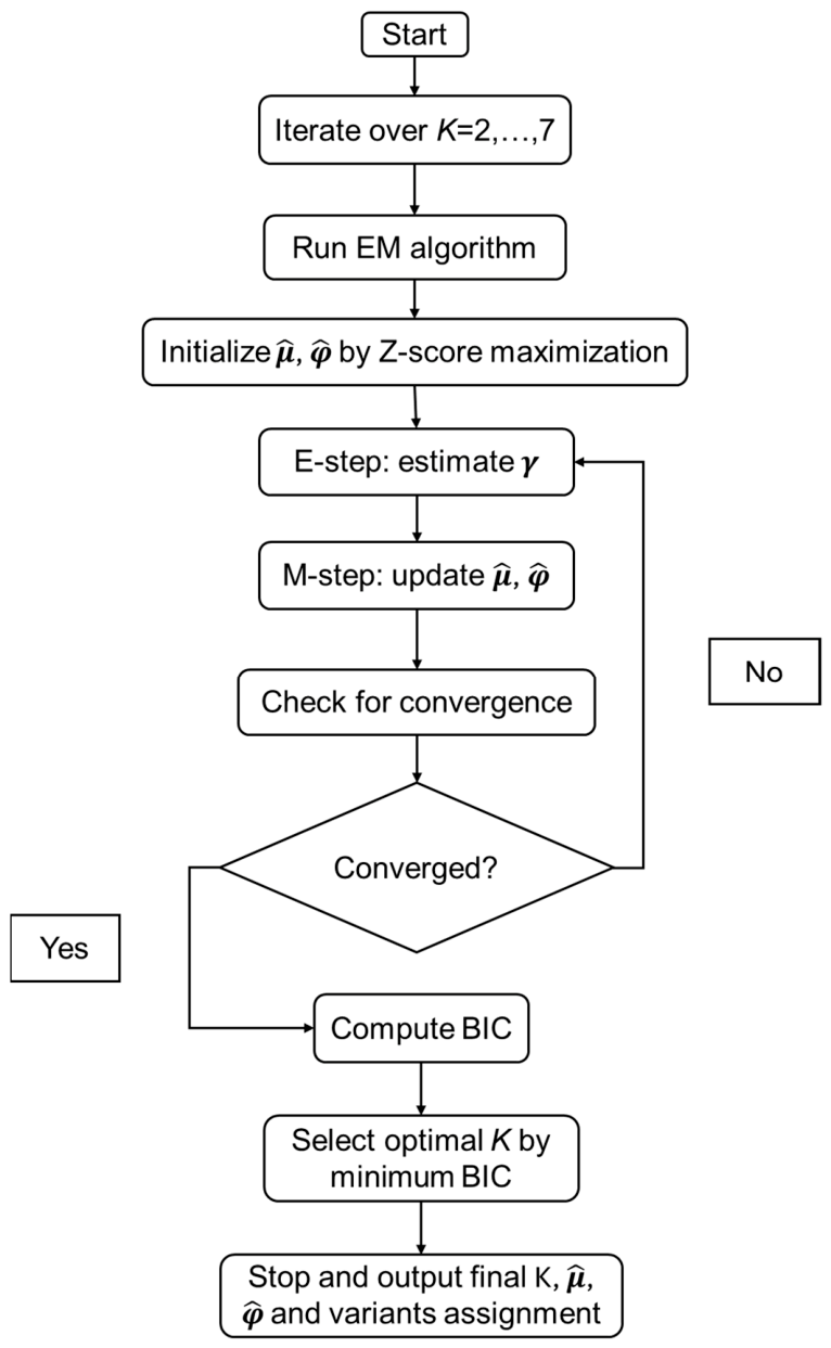
The main steps of the gvClust clustering framework are summarized in a flowchart (Figure 1). The code for this study is publicly available at https://github.com/mtDNA-BU/ClusterRare (accessed on 11 March 2025). All analyses were conducted in an R (version 4.0.5) environment, using the following computational resources: 8 GB memory per core and 4 OpenMP parallel cores.

2.5. A Simulation Study

We simulated a continuous phenotype using the following model:

$$y=10+0.6X_1+0.8X_2+{\mathit{G}}_C^T\mathit{\beta }+\epsilon$$

(11)

where 10 is the intercept, $X_1~N\left(\mathrm{0,1}\right)$, $X_2~Binomial\left(0.5\right)$, and $\epsilon ~N(0,0.49)$. ${\mathit{G}}_C^T=(G_{C1},\dots ,G_{CL})$ is a vector that includes the genetic coding for the L randomly chosen causal rare variants in the simulated region. $\mathit{\beta }={({\beta }_1,\dots ,{\beta }_L)}^{\mathit{T}}$ is a vector of the true beta effects for the selected causal variants. The beta effect of the rare variant i is based on $R^2$ and $\mathit{\omega }$. $R^2$ is the proportion of variance explained by all of the causal rare variants for a continuous trait. $\mathit{\omega }=\{{\omega }_1,\dots ,{\omega }_L\}$ is the ratio of the beta effects of each causal rare variant. The elements of $\mathit{\omega }$ are randomly assigned to each causal rare variant. ${\beta }_l=sign({\omega }_l)\sqrt{{\displaystyle \frac{c{s}_l^2}{2{MAF}_l(1-{MAF}_l)}}}$ and $c={\displaystyle \frac{R^2}{{\mathit{s}}^{T}D\mathit{s}}}$, where D is the correlation matrix between the causal variants, and $\mathit{s}=(s_1,\dots ,s_l)$, where $s_l=sign\left({\omega }_l\right)\sqrt{2{MAF}_l(1-{MAF}_l){\omega }_l^2}$. The proportion of variance (R²) explained by the causal rare variants is set to be 3% for the continuous phenotype. We also apply a cutoff of the 80% quantile to the simulated continuous phenotype, with R² = 3%, to obtain a binary phenotype. The variance explained by $X_1$, $X_2,$ and the random error are around 36%, 16%, and 45%, respectively.

We conduct a simulation study of 1000 replicates to evaluate the performance of the proposed clustering method. We generate 60 rare variants with a minor allele frequency (MAF) in 0.002 ≤ MAF < 0.01. It has been shown that rare variants display mild linkage disequilibrium (LD) between each other [18]. LD may affect the performance of the clustering because the GMM model assumes the data points are independent. To evaluate the effect of LD on rare variant clustering, we perform simulations to generate rare variants under two conditions: independent variants and those that display LD, using human genome sequence data from the 1000 Genome Project Build 37 as the reference [19]. For the first condition, we generate genotypes using the PhenotypeSimulator R package [20]. This package simulates genotypes based on the binomial distribution that does not incorporate LD. Second, we generate genotypes using the sim1000g R package that uses the first 60 rare variants in the B-Cell Translocation Gene 3 (BTG3) gene (19,249 base pairs in length, GRCh37/hg19) on chromosome 21 from the human 1000 Genomes Project (Build 37) as the reference. Of note, the choice of the BTG3 gene is arbitrary. The sim1000G package simulates variants for small or large genomic regions or a full chromosome in unrelated individuals or family data. Haplotypes are extracted to compute LD in the simulated genomic regions and to generate new genotype data among individuals. For both situations, i.e., the presence and absence of LD by the two R packages, we simulate 1000 replicates of 5000, 15,000, and 25,000 samples. To compare the effect of sample size on rare variant clustering, we randomly select 5000, 15,000, and 25,000 samples from the underlying population of 250,000 individuals. To understand the LD structure between rare variants generated by the sim1000g package, we calculate an average correlation matrix of the simulated 60 rare variants over the 1000 replicates.

For both the continuous and binary traits, we compare the performance of the clustering methods under six simulation scenarios (

Table 1. Summary of six simulation scenarios with 1000 replicates.

	Number of Groups of Rare Variants	The Ratio of the True Beta Effects Between Each Group	Proportions of the Number of Rare Variants Among Each Group
Scenario 1	3	0:1:2	${\displaystyle \raisebox{1ex}{$1$}\!\left/ \!\raisebox{-1ex}{$3$}\right.}:{\displaystyle \raisebox{1ex}{$1$}\!\left/ \!\raisebox{-1ex}{$3$}\right.}:{\displaystyle \raisebox{1ex}{$1$}\!\left/ \!\raisebox{-1ex}{$3$}\right.}$
Scenario 2	3	−1:0:1	${\displaystyle \raisebox{1ex}{$1$}\!\left/ \!\raisebox{-1ex}{$3$}\right.}:{\displaystyle \raisebox{1ex}{$1$}\!\left/ \!\raisebox{-1ex}{$3$}\right.}:{\displaystyle \raisebox{1ex}{$1$}\!\left/ \!\raisebox{-1ex}{$3$}\right.}$
Scenario 3	4	−1:0:1:2	${\displaystyle \raisebox{1ex}{$1$}\!\left/ \!\raisebox{-1ex}{$4$}\right.}:{\displaystyle \raisebox{1ex}{$1$}\!\left/ \!\raisebox{-1ex}{$4$}\right.}:{\displaystyle \raisebox{1ex}{$1$}\!\left/ \!\raisebox{-1ex}{$4$}\right.}:{\displaystyle \raisebox{1ex}{$1$}\!\left/ \!\raisebox{-1ex}{$4$}\right.}$
Scenario 4	5	−2:−1:0:1:2	${\displaystyle \raisebox{1ex}{$1$}\!\left/ \!\raisebox{-1ex}{$5$}\right.}:{\displaystyle \raisebox{1ex}{$1$}\!\left/ \!\raisebox{-1ex}{$5$}\right.}:{\displaystyle \raisebox{1ex}{$1$}\!\left/ \!\raisebox{-1ex}{$5$}\right.}:{\displaystyle \raisebox{1ex}{$1$}\!\left/ \!\raisebox{-1ex}{$5$}\right.}:{\displaystyle \raisebox{1ex}{$1$}\!\left/ \!\raisebox{-1ex}{$5$}\right.}$
Scenario 5	2	1:2	${\displaystyle \raisebox{1ex}{$1$}\!\left/ \!\raisebox{-1ex}{$2$}\right.}:{\displaystyle \raisebox{1ex}{$1$}\!\left/ \!\raisebox{-1ex}{$2$}\right.}$
Scenario 6	2	−1:1	${\displaystyle \raisebox{1ex}{$1$}\!\left/ \!\raisebox{-1ex}{$2$}\right.}:{\displaystyle \raisebox{1ex}{$1$}\!\left/ \!\raisebox{-1ex}{$2$}\right.}$

). For Scenario 1: 1/3 of the variants within the target region are non-causal, 1/3 of the variants are causal with moderate positive effects, and 1/3 of the variants are causal with strong positive effects. The ratio of moderate and strong effects is 1:2. In Scenario 2: 1/3 of the variants within the target region are non-causal, 1/3 of the variants are causal with positive effects, and 1/3 of the variants are causal with negative effects. The effect size of each causal variant is the same for this scenario. In Scenario 3: 1/4 of the variants within the target region are non-causal, 1/4 of the variants are causal with moderate positive effects, 1/4 of the variants are causal with strong positive effects, and 1/4 of the variants are causal with moderate negative effects. The ratio of the effects is −1:0:1:2 for this scenario. In Scenario 4: 1/5 of the variants within the target region are non-causal, 1/5 of the variants are causal with moderate positive effects, 1/5 of the variants are causal with strong positive effects, 1/5 of the variants are causal with moderate negative effects, and 1/5 of the variants are causal with strong negative effects. The ratio of the effects is −2:−1:0:1:2. In Scenario 5: 1/2 of the variants are causal with moderate positive effects, and the other 1/2 of the variants are causal with strong positive effects. The ratio of the effects is 1:2. In Scenario 6: 1/2 of the variants are causal with positive effects, and the other 1/2 of the variants are causal with negative effects. The ratio of the effects is −1:1. Note that Scenarios 5 and 6 are two extreme cases that do not contain a null cluster.

We adopt the adjusted Rand index [21] (ARI) method to measure the similarity between the true and predicted allocations of clusters. That is, we calculate the average ARI over the 1000 replicates to evaluate the performance of the method. The adjustedRandIndex function in mclust R package version 5.4.7 is used for the ARI calculation. For each scenario, we also calculate the accuracy of the number of clusters K* determination. The accuracy is calculated as

$$Accuracy={\displaystyle \frac{\# \mathrm{o}\mathrm{f} \mathrm{r}\mathrm{e}\mathrm{p}\mathrm{l}\mathrm{i}\mathrm{c}\mathrm{a}\mathrm{t}\mathrm{e}\mathrm{s} \mathrm{d}\mathrm{e}\mathrm{t}\mathrm{e}\mathrm{r}\mathrm{m}\mathrm{i}\mathrm{n}\mathrm{e} K^{*} \mathrm{c}\mathrm{o}\mathrm{r}\mathrm{r}\mathrm{e}\mathrm{c}\mathrm{t}\mathrm{l}\mathrm{y}}{\# \mathrm{o}\mathrm{f} \mathrm{r}\mathrm{e}\mathrm{p}\mathrm{l}\mathrm{i}\mathrm{c}\mathrm{a}\mathrm{t}\mathrm{e}\mathrm{s}}}$$

(12)

To assess the deviation between the mean effects in estimation and the “true” effects from the simulation of the clusters, we calculate the mean squared error (MSE) by

$$MSE={\displaystyle \frac{{\sum }_r{\sum }_j{({\beta }_{rj}-\widetilde{{\beta }_{rj}})}^2}{J\times \# of replicates}}$$

(13)

where ${\beta }_{rj}$ is the true mean of the j-th cluster in the r-th replicate, and $\widetilde{{\beta }_{rj}}$ is the corresponding estimated mean based on our clustering algorithm. For both simulation studies and real data analyses, we perform an analysis of variance (ANOVA) to test if the means of betas from different clusters are significantly different. We also apply the Mann–Whitney U test to evaluate if the mean of betas from a null cluster is significantly different from 0.

To demonstrate the strength of our method, we compared gvClust with two alternative clustering strategies:

(i)

k-means clustering, a widely used baseline unsupervised clustering method,

(ii)

gvClust-initial, which uses the same initialization procedure as gvClust but skips the subsequent expectation–maximization (EM) updates (i.e., clustering based solely on initialization). We compare these methods under each of the six scenarios for a continuous trait with the absence of LD and N = 25,000 individuals.

Because there are currently few established methods specifically designed for clustering genetic variants using GWAS summary statistics (e.g., effect size estimates and standard errors), k-means was chosen as a representative generic clustering approach. This comparison isolates the advantages of a model-based approach that explicitly accounts for uncertainty and heterogeneity using a Gaussian mixture model (GMM).

2.6. Application to Exome-Wide Association and a Rare-Variant GWAS of Blood Pressure Traits

To demonstrate the proposed clustering method, we apply the method to cluster the rare variants within the significant genes associated with blood pressure (BP) traits. Blood pressure is an inherited trait with an estimated heritability of up to 30–70% [22]. High blood pressure is an independent risk factor for cardiovascular diseases [23]. We apply the proposed clustering method to summary statistics obtained from the most updated association studies and meta-analysis of BP traits by Surendran et al. [14]. This study included more than 800,000 individuals from four consortia (CHARGE, CHD Exome+, GoT2D:T2DGenes, and ExomeBP) and UK BioBank data [14]. In this study, an exome-wide association (EWAS) and a rare-variant GWAS (RV-GWAS), using imputed and genotyped single nucleotide variants (SNVs), were conducted to identify common and rare variants and genes that were associated with three continuous BP traits (systolic blood pressure [SBP], diastolic blood pressure [DBP], and pulse pressure [PP]) and hypertension (HTN) by using both a single-variant model and gene-based tests. This great effort validated most of the previously identified BP-associated single variants and genes. In addition, this large study discovered several new SNVs and genes associated with BP traits [14]. To cluster rare variants, we focus on those in genes associated with SBP, DBP, PP, and HTN. We apply two strategies to cluster the rare variants. In the first strategy, we cluster rare variants within each signal gene for SBP, DBP, PP, and HTN separately. In the second strategy, for each blood trait, we combine all the signal genes and cluster all rare variants within this combined gene region.

We also annotate each rare variant with the Combined Annotation Dependent Depletion (CADD) score and consequence types using the GenomicScores R package [24]. All analyses were conducted using R (4.4.0), Posit Software, PBC. 250 Northern Ave, Boston, Massachusetts 02210, US.

3. Results

3.1. Simulation Studies

We first compared clustering methods under different scenarios using independent rare variants generated by the PhenotypeSimulator R package [20]. We then evaluated the effect of LD on the clustering method for rare variants generated by the sim1000G R package with version of 1.40.

3.1.1. Simulations Without LD Structure

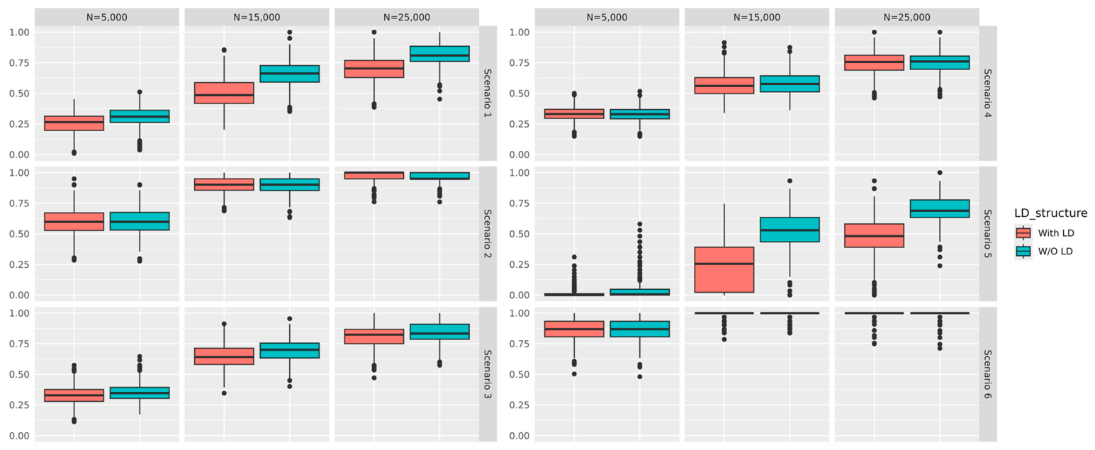
The ARI value was largely improved when the sample size was increased, indicating that a large sample size provided a more accurate allocation of the clusters. For example, with a sample size of 5000, the mean ARI value was 0.60 for the combined weighting scheme for a continuous trait under simulation Scenario 2. With a sample size of 15,000 and 25,000, the ARI value increased to 0.90 and 0.96, respectively. The ARI values were comparable using three Z-score weighting schemes under each scenario (Supplementary Figures S4 and S5). Simulation Scenarios 2 and 6 had higher mean ARI values compared to the other scenarios if other conditions were the same. This observation was as expected because the two signal clusters had opposite effect directions, and the differences between the true cluster means of the two signal clusters were larger than those of the other scenarios.

With a pre-specified number of clusters K* ranging from two to seven, the accuracy of determining the number of clusters was high (>0.9) for all simulation scenarios when the sample size reached 25,000 for a continuous trait. The MSE of the estimates for the true cluster means was reduced with the increase in sample size. The ANOVA test was significant for all replicates under each scenario (p < 0.05), indicating that the means of betas from the different clustering were significantly different. The Mann–Whitney test presented non-significant results for all the scenarios (p > 0.05), indicating that the rare variants allocated to the null cluster display effect sizes not significantly different from 0.

The ARI value of clustering for binary outcomes was lower than that of continuous outcomes when all the other conditions remained the same (Supplementary Figures S1–S11). For example, when there was no LD and the sample size was 15,000, the mean ARI value of a continuous trait with the combined weighting was 0.66 under Scenario 1. The corresponding mean ARI value of a binary trait was 0.33.

3.1.2. Comparison of Simulations with and Without LD

We observed a moderate or low LD between the 60 simulated rare variants using the sim1000g package (Supplementary Figure S1). Among a total of 1770 rare variant pairs from the 60 rare variants, 530 pairs (29.9%) displayed a correlation between 0.01 and 0.05, with 73 pairwise displaying correlations > 0.05. The strongest correlation between the two variants was 0.26. The two variants had MAFs of 0.0031 and 0.0032.

For simulation Scenarios 2, 4, and 6, the simulated genotype displaying mostly moderate LD provided comparable mean ARI values, MSEs, and accuracy of specification of the number of clusters K* compared to those of independent rare variants (Figure 2, Supplementary Figure S2). For example, the mean ARI values with/without the presence of LD among the variants were comparable (0.91 vs. 0.9) in Scenario 2, with a sample size of 15,000 for a continuous trait using the combined weighting scheme. The corresponding MSEs (0.0023 vs. 0.0022) and accuracy of specification of the number of clusters K* (0.992 vs. 0.995) were similar between the presence and absence of the LD structure. For simulation Scenarios 1, 3, and 5, the simulated genotype displaying mostly moderate LD provided a lower mean ARI value, larger MSE, and lower accuracy of specification of the number of clusters K* compared to those of independent rare variants (

Table 2. The MSEs of estimated clusters’ means for a continuous trait in simulation studies (with and without the presence of LD).

	Scenario	N = 5000	N = 15,000	N = 25,000
Without LD
	Scenario 1	0.0102	0.00329	0.00169
	Scenario 2	0.0102	0.00221	0.000868
	Scenario 3	0.0124	0.00366	0.00179
	Scenario 4	0.0127	0.00461	0.00228
	Scenario 5	0.00535	0.0024	0.00141
	Scenario 6	0.00574	0.000633	0.000143
With LD
	Scenario 1	0.0102	0.00429	0.00225
	Scenario 2	0.0118	0.00226	7.00 × 10−4
	Scenario 3	0.014	0.00446	0.0022
	Scenario 4	0.0148	0.00557	0.00268
	Scenario 5	0.00405	0.00282	0.00177
	Scenario 6	0.0061	0.00042	0.000116

MSE, mean square error; LD, linkage disequilibrium. Rare variants without LD were generated using the PhenotypeSimulator R packages based on the binomial distribution. Rare variants with LD were generated using the sim1000g R package, which uses the first 60 rare variants in the B-Cell Translocation Gene 3 (BTG3) on chromosome 21 (19,249 base pairs in length, GRCh37/hg19) from the human 1000 Genomes Project (Build 37) as the reference. The choice of the BTG3 gene is arbitrary.

, Supplementary Tables S1 and S2, and Figure 1, Supplementary Figures S4 and S5). For example, using the combined weighting scheme, in a sample size of 15,000 with a continuous trait, the average ARI value was 0.51 when the simulated rare variants displayed LD for Scenario 1. In contrast, when simulated genotypes were independent, the average ARI value was 0.66, which was about 0.14 higher than the clustering result based on the variants with LD using the same sample size. The corresponding MSE from clustering rare variants without the LD structure was 0.0033 (Table 2), while the MSE from clustering rare variants with LD was 0.0043 (Table 2). The specification accuracy of the number of K* clusters with the presence of LD (0.715) was lower than that (0.911) with the absence of LD between variants. Comparing the clustering performance of the scenarios between the presence and absence of LD, we observed that the presence of LD had a larger effect on the performance of clustering for Scenarios 1, 3, and 5 compared to Scenarios 2, 4, and 6. This was likely due to the smaller differences between the true cluster means in Scenarios 1, 3, and 5 compared to those in Scenarios 2, 4, and 6.

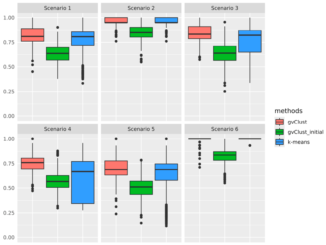
We also compared the clustering performance for gvClust, gvClust-initial, and k-means across six simulation scenarios. Overall, gvClust consistently demonstrated superior performance compared with both k-means and gvClust-initial. Across all scenarios, gvClust achieved the highest median clustering accuracy with reduced variability, indicating both improved accuracy and robustness. In contrast, k-means showed larger variability and inferior performance in most scenarios, particularly when clusters differ in variance or overlap substantially, reflecting the limitations of distance-based methods that do not incorporate summary-statistic uncertainty (Figure 3).

Notably, gvClust-initial performed systematically worse than the full gvClust procedure. While initialization alone can partially capture coarse structure in the data, the absence of EM refinement leads to suboptimal and more variable clustering. This performance gap clearly demonstrates the importance of the iterative E- and M-steps in gvClust, which jointly leverage effect sizes and standard errors to refine cluster membership and parameter estimates. In scenarios with stronger signal separation (e.g., Scenario 2 and Scenario 6), all methods performed relatively well; however, gvClust still attained near-optimal performance with minimal dispersion. In more challenging settings (Scenarios 1, 3, 4, and 5), the areas contained weaker signals and exhibited greater heterogeneity among the variants; gvClust substantially outperformed both alternatives, highlighting its robustness in realistic GWAS contexts. Collectively, these results confirm that the performance gains of gvClust come from its full model-based EM framework, which explicitly accounts for uncertainty in genetic effect estimation, rather than solely from its initialization scheme.

3.2. Application to a GWAS on BP Traits with Rare Variants

3.2.1. Identification of Blood Pressure Trait-Associated Genes

Using the SKAT test, multiple rare variants (MAF < 0.01) were identified for one or more BP traits (p < 2.5 × 10⁻⁶) with four genes (NPR1, DBH, COL21A1, and NOX4) [14,25]. Low frequency and rare variants in two additional genes, PLCB3 and CEP120, were associated with BP traits at MAF < 0.05. The six genes harbor different numbers of rare variants. More specifically, NPR1 included 13 rare variants, DBH included 29 rare variants, COL21A1 included 26 rare variants, and NOX4 included nine rare variants (Supplementary Table S3). SBP was associated with NPR1, DBH, and PLCB3; DBP was associated with DBH and PLCB3; and PP was associated with COL21A1, NOX4, and CEP120 due to multiple rare variants in the gene (p < 2.5 × 10⁻⁶). Because gene-based test results were not available for the associations between HTN and these six genes in the GWAS [14], we defined a signal gene for HTN if any of the six genes contained rare variant(s) (MAF < 0.01) with p < 1 × 10⁻⁴ in the single-variant HTN association testing. The three genes DBH, NPR1, and PLCB3 included rare variant(s), displaying association with HTN at p < 1 × 10⁻⁴. We applied the proposed clustering method to cluster BP-associated rare variants in these genes.

3.2.2. Annotation of Rare Variants Within Blood Pressure Trait-Associated Genes

By using the GenomicScores R package, we annotated all the rare variants in the blood pressure trait-associated genes (Supplementary Tables S7–S21). Most of the variants were classified as missense variants, and most of them had a CADD score larger than or equal to 20.

3.2.3. Clustering of Rare Variants

For the first clustering strategy, we performed rare variant clustering in eleven gene-trait associations (six genes with four traits): three genes associated with SBP, two genes associated with DBP, three genes associated with PP, and three genes that contain significant rare variants with HTN. On average, a signal gene contains about 20 rare variants. Two to three clusters were identified in each of the eleven gene-trait associations. About 70% of the rare variants were clustered into a null cluster (

Table 3. A summary of clustering results for rare variants within the combined signal regions of BP traits.

Trait	# Variants	# Clusters	Mu	Phi	# Variants in Clusters	p-Value ANOVA	p-Value MWU
SBP	58	3	0/−0.0826/0.0573	0.719/0.178/0.102	46/8/4	4.26 × 10−18	0.559
DBP	45	3	0/−0.0924/0.0471	0.718/0.165/0.117	37/5/3	1.68 × 10−11	0.338
PP	55	5	0/−0.0438/−0.0968/0.334/0.173	0.673/0.134/0.0654/0.0313/0.0966	43/4/2/1/5	1.39 × 10−19	0.976
HTN	59	3	0/−2.785/4.646	0.802/0.147/0.0516	48/8/3	3.66 × 10−16	0.32

SBP, systolic blood pressure; DBP, diastolic blood pressure; PP, pulse pressure; HTN, hypertension; Mu, the mean effect sizes of the identified clusters; Phi, the proportion of rare variants in each cluster; MWU, Mann–Whitney U test.

and

Table 4. A summary of clustering results for rare variants within the signal genes for SBP.

Gene	Chr	Start (bp)	End (bp)	# Variants	# Clusters	Mu	Phi	# Variants in Clusters	p-Value _ANOVA	p-Value MWU
DBH	9	136501569	136523555	27	2	0/−0.082	0.75/0.25	21/6	5.18 × 10−8	0.785
NPR1	1	153652129	153665650	13	3	0/−0.0846/0.164	0.727/0.198/0.0753	10/2/1	6.02 × 10−5	0.322
PLCB3	11	64021930	64034975	18	2	0/0.0529	0.716/0.284	15/3	2.33 × 10−5	0.934

DBH, dopamine beta-hydroxylase; NPR1, natriuretic Peptide Receptor 1; PLCB3, phospholipase C Beta 3; Mu, the mean effect sizes of the identified clusters; Phi, the proportion of rare variants in each cluster; MWU, Mann–Whitney U test.

, Supplementary Tables S4–S21). For example, the NPR1 gene contained 12 rare variants. We identified three clusters of rare variants in this gene for the HTN association. The means of standardized beta coefficients (z-scores) were significantly different across the three clusters (ANOVA p = 0.00028). Of the 12 rare variants, eight variants were in the null cluster. The rare variants allocated to the null cluster displayed effect sizes (i.e., the standardized beta coefficients) not significantly different from zero (Mann–Whitney U test p = 0.46). Three variants, including rs140425746, rs61757359, and rs61758562, were grouped into a cluster with an average effect size of −2.05. The rare variant, rs116245325, which displayed the smallest p-value of 1.46 × 10⁻⁵ with HTN in single variant analysis, forms a single cluster with an effect size of 4.33. Of note, the clustering pattern in this example was similar to the layout of Scenario 2 in the simulation study. That is, the two signal clusters had opposite effect directions. (Supplementary Tables S20 and S21).

For the second clustering strategy, we conducted clustering analyses on the combined summary data from significant genes that were associated with each of the BP traits. Three genes were associated with PP traits. (Supplementary Table S3) A total of 55 variants were located in these three genes. Of the 55 rare variants within these three genes, we identified five clusters with distinct effect sizes (ANOVA p = 1.39 × 10⁻¹⁹). (Table 3, Supplementary Table S9) The null cluster contained 43 out of 55 variants. The effect sizes of rare variants allocated to the null cluster displayed were not significantly different from zero (Mann–Whitney U test p = 0.976). Two rare variants, rs139341533 and rs56061986, were clustered together with an average effect size of −0.097. Four rare variants, rs2303720, rs114280473, rs189429890, and rs144215891, were assigned to a distinct cluster with an average effect size of −0.0438. A single variant, rs200999181, was recognized as the only variant in the cluster with the strongest effect size of 0.334. Five rare variants, rs201955087, rs115079907, rs76146749, rs200401514, and rs2764043, were grouped into a signal cluster with a moderate positive effect size of 0.173. The observed five-cluster pattern was similar to that in Scenario 4 of the simulation study (Table 1). Of note, Scenario 4 included four signal clusters: one with a strong positive effect, one with a moderate positive effect, one with a strong negative effect, and one with a moderate negative effect. For both positive and negative effects, the clusters with strong effect sizes were twice the size of those with moderate effect sizes. The number of variants within the moderate effect size clusters was greater than that within the strong effect size clusters. Additionally, the effect size of positive associations was larger than that of negative associations.

3.3. Computational Burden

The simulation study took a total of 16.7 h with four cores and 8 Gb of memory for each core (Supplementary Table S22). The real data analysis took around 41 s with one core of 4GB of memory.

4. Discussion

We proposed a new method to cluster rare variants within signal gene regions associated with disease traits based on summary statistics of variant–trait associations. We performed a comprehensive simulation study to evaluate the performance of the proposed method under different scenarios concerning variant effect direction, LD structure, the number of clusters, and the study sample size. In simulation Scenarios 1, 3, and 5, we observed that the proposed method provided a higher ARI value, a lower MSE, and a higher accuracy in the specification of the number of clusters with rare variants in the absence of LD, compared to those with low LD, given that the other conditions are the same. This is expected because the GMM model assumes that the data points (i.e., rare variants) are independent. The ARI value is improved, and the MSE value is decreased with an increase in sample size. Among the simulated scenarios, Scenario 2 yielded the highest ARI value, smallest MSE, and highest accuracy in the specification K* clusters because this scenario had the largest differences between the true means between clusters.

We also applied the proposed method to cluster rare variants in signal genes associated with BP traits using summary statistics from a large GWAS and meta-analysis of BP traits using around 1.3 million individuals [14]. We first classified the rare variants in individual genes per trait. To further demonstrate the classification utility, we applied the methods with combined variants in several genes that are associated with the same traits. We found that most of the rare variants within the BP traits-associated genes are grouped into the null cluster, indicating that natural selection is likely the main force in shaping the rare variants in the human genome [26]. In addition, we found that rarer variants were allocated to clusters with negative means than those with positive means.

Gene-based tests, such as the burden test, SKAT, and ACAT-O, are designed to evaluate the aggregate effects of rare variants [4,6,27]. Recent work has also extended rare variant analysis in several directions, including annotation-informed testing, noncoding rare variant analysis, large-scale meta-analysis, and summary-statistic approaches for detecting allelic series [7,8,9,10,11]. These methods have improved association testing and interpretation; however, a common limitation of these gene-based tests is their inability to cluster possibly null, risk, or protective rare variants in trait-associated regions. Motivated by a clustering algorithm used in Mendelian randomization (MR) [28], our method offers a key advantage by classifying rare variants into signal and non-signal variants specific to disease traits. Our approach enables more accurate identification of true genetic signals by distinguishing variants with opposite effects or varying effect sizes. Additionally, it can integrate various annotations to prioritize signal variants, improving the accuracy of association testing and enhancing the detection of relevant genetic factors. Furthermore, our method is computationally efficient for large-scale sequencing data analysis.

Previous studies have reported inconsistent views about the LD structure among rare variants, with some assuming independence and others a mild correlation between rare variants [18]. Ignoring LD may introduce bias or loss of power in the association testing of the rare variants. In this study, we conducted simulations using independent rare variants and those based on a genomic region on chromosome 21. We found that 65% of simulated rare variants had no LD (R² < 0.01), 32% displayed low pairwise LD (R² between 0.01 and 0.05), and about 4.5% showed R² in 0.05–0.33. We evaluated the robustness of our algorithm in a simulation study with two analyses: rare variants with and without LD. The method performs better with independent rare variants, particularly when cluster means are similar, even when the multiple-variant model accounts for LD. Our method yielded more false-positive findings for variants with LD in most scenarios compared to those without LD, especially for smaller sample sizes (Table 2). However, the algorithm performs well with variants containing LD when the sample size is large enough (N = 25,000). Additionally, the multiple-variant model requires individual-level genotype data, making it more cost-effective to extend our algorithm to use summary data from large GWASs, which could enhance robustness and reduce false positives in clustering. Related work in other areas has also considered reducing the influence of noisy observations during iterative fitting, such as PSSCL, which uses progressive sample selection in a noisy-label learning framework [29].

In summary, the proposed clustering algorithm identifies risk and/or protective rare variants of distinct magnitudes according to summary statistics of SNP-trait associations. The proposed method can be easily applied to summary statistics from emerging large-scale rare variant GWASs to identify and group trait-associated rare variants into null and signal groups of discrete effect magnitudes. Therefore, this proposed method may facilitate the identification of potentially causal rare variant clusters in genomic regions and ultimately help understand the genetic architecture underlying human complex traits for the discovery of drug targets and the design of gene therapy.

References

1. Visscher, P.M.; Wray, N.R.; Zhang, Q.; Sklar, P.; McCarthy, M.I.; Brown, M.A.; Yang, J. 10 Years of GWAS Discovery: Biology, Function, and Translation. Am. J. Hum. Genet. 2017, 101, 5–22. [Google Scholar] [CrossRef] [PubMed]
2. Zuk, O.; Schaffner, S.F.; Samocha, K.; Do, R.; Hechter, E.; Kathiresan, S.; Daly, M.J.; Neale, B.M.; Sunyaev, S.R.; Lander, E.S. Searching for missing heritability: Designing rare variant association studies. Proc. Natl. Acad. Sci. USA 2014, 111, E455–E464. [Google Scholar] [CrossRef] [PubMed]
3. Li, B.; Lea, S.M. Methods for detecting associations with rare variants for common diseases: Application to analysis of sequence data. Am. J. Hum. Genet. 2008, 83, 311–321. [Google Scholar] [CrossRef]
4. Wu, M.C.; Lee, S.; Cai, T.; Li, Y.; Boehnke, M.; Lin, X. Rare-variant association testing for sequencing data with the sequence kernel association test. Am. J. Hum. Genet. 2011, 89, 82–93. [Google Scholar] [CrossRef]
5. Lee, S.; Wu, M.C.; Lin, X. Optimal tests for rare variant effects in sequencing association studies. Biostatistics 2012, 13, 762–775. [Google Scholar] [CrossRef]
6. Liu, Y.; Chen, S.; Li, Z.; Morrison, A.C.; Boerwinkle, E.; Lin, X. ACAT: A Fast and Powerful p Value Combination Method for Rare-Variant Analysis in Sequencing Studies. Am. J. Hum. Genet. 2019, 104, 410–421. [Google Scholar] [CrossRef]
7. Clarke, B.; Holtkamp, E.; Öztürk, H.; Mück, M.; Wahlberg, M.; Meyer, K.; Munzlinger, F.; Brechtmann, F.; Hölzlwimmer, F.R.; Lindner, J.; et al. Integration of variant annotations using deep set networks boosts rare variant association testing. Nat. Genet. 2024, 56, 2271–2280. [Google Scholar] [CrossRef] [PubMed]
8. Ziyatdinov, A.; Mbatchou, J.; Marcketta, A.; Backman, J.; Gaynor, S.; Zou, Y.; Joseph, T.; Geraghty, B.; Herman, J.; Watanabe, K.; et al. Joint testing of rare variant burden scores using non-negative least squares. Am. J. Hum. Genet. 2024, 111, 2139–2149. [Google Scholar] [CrossRef]
9. Kim, Y.; Jeong, M.; Koh, I.G.; Kim, C.; Lee, H.; Kim, J.H.; Yurko, R.; Bin Kim, I.; Park, J.; Werling, D.M.; et al. CWAS-Plus: Estimating category-wide association of rare noncoding variation from whole-genome sequencing data with cell-type-specific functional data. Brief. Bioinform. 2024, 25, bbae323. [Google Scholar] [CrossRef]
10. Park, E.; Nam, K.; Jeong, S.; Keat, K.; Kim, D.; Bansal, V.; Zhou, W.; Lee, S. Scalable and accurate rare variant meta-analysis with Meta-SAIGE. Nat. Genet. 2025, 57, 3185–3192. [Google Scholar] [CrossRef]
11. McCaw, Z.R.; Gao, J.; Dey, R.; Tucker, S.; Zhang, Y.; Gronsbell, J.; Li, X.; Fox, E.; O’DUshlaine, C.; Soare, T.W. A scalable framework for identifying allelic series from summary statistics. Am. J. Hum. Genet. 2025, 112, 2772–2788. [Google Scholar] [CrossRef] [PubMed]
12. McLachlan, G.J.; Peel, D. Finite Mixture Models. In Probability and Statistics—Applied Probability and Statistics Section; Wiley: New York, NY, USA, 2000; Volume 299. [Google Scholar]
13. McLachlan, G.J.; Krishnan, T. The EM Algorithm and Extensions; Wiley: New York, NY, USA, 1996. [Google Scholar]
14. Surendran, P.; Feofanova, E.V.; Lahrouchi, N.; Ntalla, I.; Karthikeyan, S.; Cook, J.; Chen, L.; Mifsud, B.; Yao, C.; Kraja, A.T.; et al. Discovery of rare variants associated with blood pressure regulation through meta-analysis of 1.3 million individuals. Nat. Genet. 2020, 52, 1314–1332. [Google Scholar] [CrossRef]
15. Dempster, A.P.; Laird, N.M.; Rubin, D.B. Maximum Likelihood from Incomplete Data via the EM Algorithm. J. R. Stat. Soc. B 1977, 39, 1–38. [Google Scholar] [CrossRef]
16. Lloyd, S. Least squares quantization in PCM. IEEE Trans. Inf. Theory 1982, 28, 129–137. [Google Scholar] [CrossRef]
17. MacQueen, J. Multivariate observations. In Proceedings of the 5th Berkeley Symposium on Mathematical Statistics and Probability, Berkeley, CA, USA, 21 June–28 July 1967; University of California Press: Oakland, CA, USA, 1967. [Google Scholar]
18. Turkmen, A.; Lin, S. Are rare variants really independent? Genet. Epidemiol. 2017, 41, 363–371. [Google Scholar] [CrossRef] [PubMed]
19. The 1000 Genomes Project Consortium. A global reference for human genetic variation. Nature 2015, 526, 68–74. [Google Scholar] [CrossRef]
20. Meyer, H.V.; Birney, E. PhenotypeSimulator: A comprehensive framework for simulating multi-trait, multi-locus genotype to phenotype relationships. Bioinformatics 2018, 34, 2951–2956. [Google Scholar] [CrossRef]
21. Hubert, L.; Arabie, P. Comparing partitions. J. Classif. 1985, 2, 193–218. [Google Scholar] [CrossRef]
22. Ehret, G.B.; Caulfield, M.J. Genes for blood pressure: An opportunity to understand hypertension. Eur. Heart J. 2013, 34, 951–961. [Google Scholar] [CrossRef]
23. Forouzanfar, M.H.; Liu, P.; Roth, G.A.; Ng, M.; Biryukov, S.; Marczak, L.; Alexander, L.; Estep, K.; Abate, K.H.; Akinyemiju, T.F.; et al. Global Burden of Hypertension and Systolic Blood Pressure of at Least 110 to 115 mm Hg, 1990-2015. JAMA 2017, 317, 165–182. [Google Scholar] [CrossRef] [PubMed]
24. Puigdevall, P.; Castelo, R. GenomicScores: Seamless access to genomewide position-specific scores from R and Bioconductor. Bioinformatics 2018, 34, 3208–3210. [Google Scholar] [CrossRef]
25. Liu, C.; Kraja, A.T.; Smith, A.J.; Brody, J.A.; Franceschini, N.; Bis, J.C.; Rice, K.; Morrison, A.C.; Lu, Y.; Weiss, S.; et al. Meta-analysis identifies common and rare variants influencing blood pressure and overlapping with metabolic trait loci. Nat. Genet. 2016, 48, 1162–1170. [Google Scholar] [CrossRef] [PubMed]
26. Bomba, L.; Walter, K.; Soranzo, N. The impact of rare and low-frequency genetic variants in common disease. Genome Biol. 2017, 18, 77. [Google Scholar] [CrossRef]
27. Lee, S.; Abecasis, G.R.; Boehnke, M.; Lin, X. Rare-variant association analysis: Study designs and statistical tests. Am. J. Hum. Genet. 2014, 95, 5–23. [Google Scholar] [CrossRef] [PubMed]
28. Foley, C.N.; Mason, A.M.; Kirk, P.D.W.; Burgess, S. MR-Clust: Clustering of genetic variants in Mendelian randomization with similar causal estimates. Bioinformatics 2021, 37, 531–541. [Google Scholar] [CrossRef] [PubMed]
29. Zhang, Q.; Zhu, Y.; Cordeiro, F.R.; Chen, Q. PSSCL: A progressive sample selection framework with contrastive loss designed for noisy labels. Pattern Recognit. 2025, 161, 111284. [Google Scholar] [CrossRef]
Figure 1. A flowchart of the gvClust clustering framework.
Algorithms 19 00426 g001
Figure 2. Boxplots of ARI values of simulation Scenarios 1, 2, 3, 4, 5, and 6 with a combined weighting scheme with/without LD for a continuous trait. See Table 1 for simulation details.
Algorithms 19 00426 g002
Figure 3. Boxplots of ARI values of simulation Scenarios 1–6 for the comparison of gvClust, initialization of gvClust, and K-means methods with the absence of LD for a continuous trait and N = 25,000. Equal weight is used for gvClust and gvClust_initial.
Algorithms 19 00426 g003