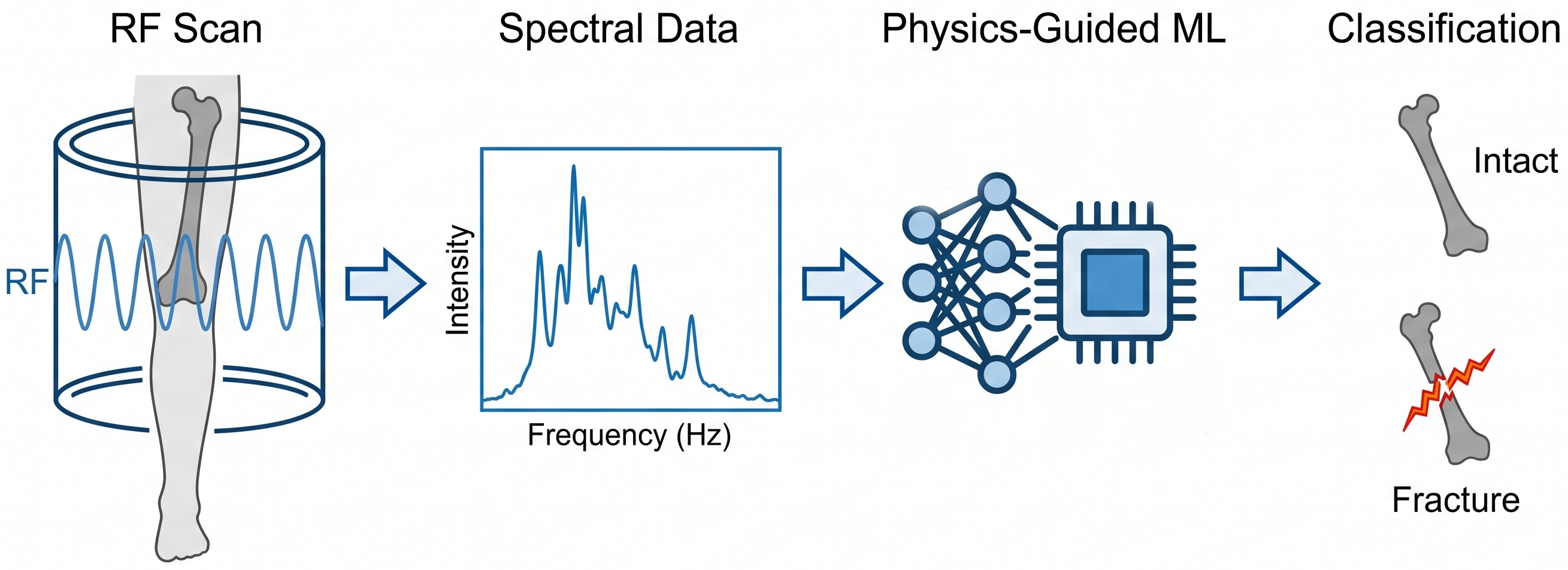
A Physics-Guided Machine Learning Algorithm for Non-Ionizing Femur Fracture Classification from RF Spectral Data

Abstract

This paper presents a physics-guided machine learning algorithm for classifying femur fracture presence and subtype using non-ionising radiofrequency (RF) spectral data. Multi-sensor S-parameter responses were generated from a femur phantom model across 1.0–3.0 GHz, producing 104 specimens representing intact bone and three fracture geometries. An exploratory, effect-size-driven band-selection algorithm identified a compact discriminative region between 1.74 and 1.90 GHz. Interpretable classifiers, including k-nearest neighbours (KNN), decision trees, linear discriminant analysis, and Naïve Bayes, were evaluated under strict specimen-level hold-out protocols to prevent data leakage. The KNN algorithm achieved 99.3% frame-level accuracy and 100% specimen-level accuracy for binary fracture detection while maintaining strong robustness in multiclass subtype classification, validated through sensor ablation and leave-one-subtype-out testing. The results demonstrate that compact, interpretable algorithms operating on band-limited RF spectra can achieve reliable, radiation-free fracture classification, supporting future development of continuous and edge-deployable monitoring systems.

1. Introduction

Bone fracture healing is a complex, multi-stage biological process encompassing inflammation, callus formation, mineralisation, and remodelling. Accurate and timely assessment is essential to prevent delayed union or non-union and to guide rehabilitation strategies [1,2,3]. In current clinical practice, fracture healing is primarily evaluated using radiographic imaging techniques such as X-ray and computed tomography (CT), supplemented by manual clinical examination [4,5]. While these approaches are effective for assessing gross structural alignment, they suffer from inherent limitations, including exposure to ionising radiation, intermittent measurement schedules, and subjective interpretation [5,6]. Consequently, clinically relevant changes in the healing trajectory may remain undetected between imaging sessions, potentially delaying intervention [6].

Non-ionising sensing technologies have therefore attracted increasing attention as potential alternatives for continuous and objective fracture monitoring [7,8]. Among these, radiofrequency (RF) and microwave sensing techniques exploit changes in the dielectric properties of biological tissues associated with fracture gaps, callus formation, and progressive mineralisation [9,10,11]. Variations in electromagnetic scattering and impedance characteristics provide indirect yet sensitive markers of tissue composition and bone integrity, a principle that has been successfully applied in a range of biomedical sensing applications [10,11,12,13]. However, RF spectral measurements are inherently high-dimensional and are strongly influenced by sensor configuration, tissue heterogeneity, and environmental clutter, making robust algorithmic interpretation a critical challenge [14,15].

Recent studies have demonstrated the feasibility of applying machine learning (ML) and deep learning (DL) methods to RF-based fracture detection, reporting high classification accuracies in controlled phantom environments [16,17]. Despite these encouraging results, several methodological limitations persist. Many existing approaches rely on broadband spectral features without physically motivated frequency selection, leading to increased dimensionality, reduced signal-to-noise ratio, and heightened susceptibility to overfitting [18,19]. Other studies evaluate performance at the frame or frequency-sample level, which can introduce data leakage when measurements from the same specimen appear in both training and testing sets, resulting in overly optimistic performance estimates [20,21]. Furthermore, the reliance on complex black-box models often limits interpretability and complicates deployment on resource-constrained or edge devices [22,23].

To address these limitations, this work proposes a physics-guided machine learning framework for RF-based femur fracture classification. The proposed approach explicitly links electromagnetic spectral behaviour to feature selection through effect-size-driven frequency band localisation [24,25], enforces strict specimen-level validation protocols to ensure robust generalisation [20,21], and prioritises interpretable baseline classifiers that are computationally efficient and suitable for edge deployment [22,23]. In addition, robustness is systematically evaluated through sensor ablation and leave-one-subtype-out (LOSO) generalisation analysis, providing insight into sensitivity to sensor configuration and fracture geometry [24].

The main contributions of this study are summarised as follows:

• A quantitative, effect-size-based band selection algorithm for identifying fracture-discriminative RF frequency regions.
• A leakage-free validation framework for binary and multiclass fracture classification using strict specimen-level and LOSO evaluation protocols.
• A comprehensive robustness analysis incorporating sensor ablation and subtype-level generalisation to assess algorithm stability and transferability.

2. Related Work

Bone fracture healing is a complex, multi-stage biological and mechanical process involving inflammation, soft callus formation, mineralisation, and remodelling. Mechanobiological computational models have been widely used to study these stages and their sensitivity to biological parameters. Mechanistic simulations of human bone fracture healing have shown that persistent inflammation significantly delays callus formation, while stiffer and less permeable granulation tissue combined with a balanced cytokine response accelerates bony bridging and union [26]. Although such studies do not employ machine learning, they provide critical biological grounding for stage-based healing classification. Furthermore, they help justify the physical interpretation of non-imaging biomarkers, such as changes in mechanical or electromagnetic properties that RF-based systems may capture indirectly.

Beyond modelling, experimental studies have demonstrated that mechanical state is a meaningful longitudinal biomarker of healing. Battery-free, implant-adjacent wireless strain sensors have been developed to monitor callus mechanics during rehabilitation, with in vivo measurements correlating strongly with micro-CT-derived bridging and histological outcomes [27]. These findings validate the concept that continuous, non-imaging sensing can reflect real-time healing progression. RF sensing of bone, particularly through changes in scattering or impedance characteristics, can be viewed as a complementary modality that probes tissue evolution through electromagnetic rather than mechanical contrast.

Implant-integrated bioelectrical sensing has further reinforced this paradigm. Smart bone plates incorporating electrical impedance spectroscopy (EIS) have been shown to track fracture healing in vivo, with impedance parameters evolving alongside tissue composition and correlating with μCT-based union metrics [28]. While EIS operates at lower frequencies than microwave sensing, both approaches exploit frequency-dependent interactions between electromagnetic fields and biological tissues. These studies therefore provide strong conceptual support for using RF S-parameters as indicators of healing state.

At higher frequencies, radio-frequency and microwave techniques have been increasingly explored for bone fracture detection and assessment. A comprehensive review of low-frequency microwave RF approaches highlighted the sensitivity of microwave signals to discontinuities and dielectric contrasts in bone and summarised early machine learning and deep learning methods applied to RF features [29]. The review also emphasised common pitfalls, including overfitting and limited dataset sizes, which are particularly relevant when transitioning from controlled phantoms to clinical deployment.

Several hardware-focused studies have sought to optimise RF sensor designs for bone applications. A notable example is the development of a dual-polarised microwave sensor based on reactive impedance surfaces, demonstrating enhanced sensitivity to fracture-induced discontinuities around 2.45 GHz in phantom and human-arm-like setups [30]. Such work directly informs RF front-end design choices, including operating frequency, polarisation diversity, and sensor geometry, that underpin reliable S-parameter acquisition.

On the algorithmic side, deep learning has been applied directly to microwave S-parameter data for fracture classification. Feed-forward deep neural networks trained on concatenated and normalised S-parameter features have reported accuracies approaching 99% on phantom datasets in the 2–3 GHz range [31]. While these results highlight the discriminative power of RF features, they also underscore the need for cautious interpretation, given the controlled nature of phantom experiments and the absence of true longitudinal healing data.

More broadly, surveys of deep learning for radio-based human sensing have provided methodological guidance on representing RF data for learning, including treating frequency responses as images, sequences, or hybrid feature sets, and mapping them to CNN, RNN, or transformer-based architectures [32]. These insights are directly applicable to RF S-parameter-based bone sensing and motivate exploration beyond simple multilayer perceptrons toward models that better exploit spectral and temporal structure.

From a clinical AI perspective, multiple reviews have examined fracture detection across imaging modalities, reporting diagnostic accuracies often exceeding 90% while highlighting persistent challenges related to dataset bias, validation rigour, and interpretability [33]. Although predominantly image-based, these studies provide valuable guidance on evaluation protocols, metric reporting, and deployment considerations that are equally applicable to RF-based systems.

Closer to the present work, concept and demonstration studies integrating RF sensing with machine learning have proposed end-to-end pipelines for monitoring and staging bone healing. These approaches combine RF-derived features with classical machine learning models such as random forests, support vector machines, and gradient boosting, as well as temporal models including LSTM and GRU networks, achieving high reported accuracies on simulated or controlled datasets. Such studies effectively serve as blueprints for RF-enabled, AI-driven healing assessment, including recommendations for ablation studies, feature comparisons, and temporal modelling.

Finally, clinical outcome prediction studies using tabular machine learning have demonstrated the feasibility of forecasting failed healing or non-union after fracture surgery using registry data. For example, XGBoost-based models trained on large clinical datasets have achieved area-under-the-curve values around 0.8 and identified clinically meaningful predictors of non-union. While not RF-based, these works illustrate best practices for clinical validation, feature importance analysis, and translational framing, informing how RF-derived biomarkers might ultimately be integrated into broader clinical decision-support systems.

An overview of the complete algorithmic pipeline, from CST-based RF simulation to band-selected machine learning classification, is shown in Figure 1.

3. Materials and Methods

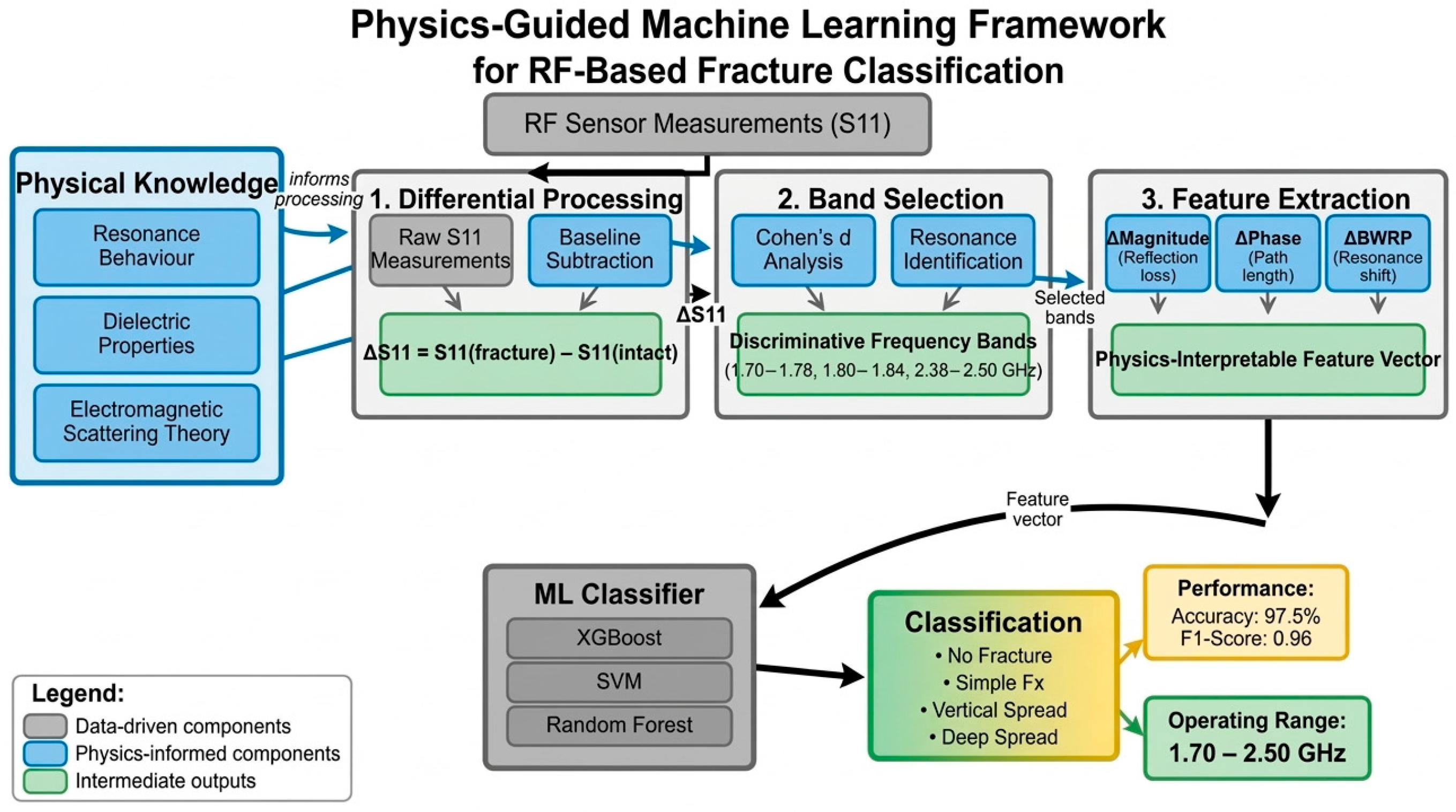
3.1. Physics-Guided Machine Learning Framework

This section establishes the conceptual foundation for the physics-guided approach employed in this study, clarifying how electromagnetic principles inform and constrain the machine learning pipeline.

3.1.1. Concept of Physics-Guided Machine Learning

Physics-guided machine learning (PGML) refers to the integration of domain-specific physical knowledge into data-driven algorithms to improve accuracy, interpretability, and generalisation. Unlike purely data-driven approaches that treat the learning problem as a black box, PGML leverages known physical relationships to:

• Constrain the hypothesis space: Physical laws reduce the set of plausible models, mitigating overfitting and improving sample efficiency.
• Guide feature engineering: Physics-informed features capture causally relevant information rather than spurious correlations.
• Enhance interpretability: Model decisions can be traced to physically meaningful quantities.
• Improve generalisation: Features grounded in physical principles are more likely to transfer across experimental conditions.

In the context of RF-based fracture classification, the physics-guided approach manifests at three stages of the algorithmic pipeline, as illustrated in Figure 2.

3.1.2. Physical Basis of RF Fracture Sensing

The detection of bone fractures using RF sensing relies on the interaction between electromagnetic waves and biological tissues with distinct dielectric properties shown in

Table 1. Dielectric properties of biological tissues and fracture gap contents at 1.8 GHz.

Tissue/Medium	Relative Permittivity (ε’)	Conductivity σ (S/m)	Loss Tangent (tan δ)
Cortical bone	12.4	0.39	0.28
Cancellous bone	18.7	0.59	0.32
Bone marrow	5.5	0.10	0.16
Blood	58.3	1.32	0.20
Muscle	54.8	1.21	0.20
Fat	5.3	0.05	0.08
Air	1.0	0.00	0.00

. The fundamental physical principles are:

(A) 

Dielectric Contrast. Different tissues exhibit characteristic complex permittivity values (${\mathit{ϵ}}^{\ast }={\mathit{ϵ}}^{\prime }-\mathit{j}{\mathit{ϵ}}^{″}$) that determine their interaction with electromagnetic fields. Table 1 summarises the dielectric properties of relevant tissues at the operating frequency range.

A fracture gap filled with blood (ε’ ≈ 58) or air (ε’ ≈ 1) introduces a substantial dielectric discontinuity relative to intact cortical bone (ε’ ≈ 12), producing measurable perturbations in the electromagnetic scattering response.

(B) 

Electromagnetic Scattering. When an RF wave encounters a dielectric discontinuity (fracture), a portion of the incident energy is reflected, transmitted, or scattered depending on the geometry and dielectric contrast. The scattering behaviour is captured by the S-parameter matrix, where changes in $S_{ij}(f)$ encode information about the discontinuity’s location, size, and composition.

(C) 

Resonance Behaviour. The sensor-phantom system exhibits frequency-dependent resonance characteristics determined by the effective electrical length of the propagation paths. Near resonance frequencies, the system is maximally sensitive to impedance perturbations, amplifying the effect of fracture-induced dielectric changes. This resonance enhancement is the physical basis for the observed concentration of discriminative information within a narrow frequency band.

3.1.3. Mapping Physical Phenomena to Algorithmic Components

Table 2. Mapping between physical phenomena and algorithmic components.

Physical Phenomenon	Algorithmic Component	Implementation	Section Reference
Static tissue scattering	Differential processing	Subtraction of NoFracture reference spectrum	Section 3.3
Dielectric contrast at fracture	Feature magnitude	Band-binned mean values capture amplitude changes	Section 3.5
Resonance frequency sensitivity	Band selection	Effect-size analysis identifies resonance region	Section 3.4
Frequency-dependent scattering	Slope features	Linear trend captures spectral shape changes	Section 3.5
Fracture geometry effects	Multiclass discrimination	Different geometries produce distinct spectral signatures	Section 4
Sensor spatial sensitivity	Channel consolidation	Receiving-port grouping preserves spatial information	Section 3.2

explicitly maps the physical phenomena to corresponding algorithmic components in the proposed pipeline.

3.1.4. Physical Interpretation of Feature Types

Each extracted feature type corresponds to a specific physical quantity:

(A) Band-Binned Mean Values. These features capture the average amplitude of the differential S-parameter response within frequency sub-bands. Physically, they reflect the magnitude of impedance perturbation caused by the fracture, which depends on:

• Fracture gap width (larger gaps → greater perturbation)
• Fracture gap contents (blood vs. air → different dielectric contrast)
• Fracture depth (deeper penetration → more tissue interaction)

(B) Statistical Descriptors (Min, Max, Std). These features characterise the extrema and variability of the spectral response:

• Minimum: Corresponds to the deepest point of the resonance notch, sensitive to fracture severity
• Maximum: Corresponds to the recovery peak, sensitive to fracture extent
• Standard deviation: Captures spectral variability, sensitive to fracture complexity

(C) Slope Features. The linear trend of the spectral response within the band reflects frequency-dependent scattering behaviour:

• Positive slope: Indicates spectral recovery following a notch, characteristic of localised fractures
• Negative slope: Indicates progressive attenuation, characteristic of extended fractures
• Slope magnitude: Correlates with the sharpness of resonance features

(D) Area Under Curve (AUC). Integrates the total spectral response, providing a global measure of dielectric perturbation that is robust to local variations.

3.1.5. Physics-Guided Constraints in the Pipeline

The physics-guided approach imposes the following constraints on the ML pipeline:

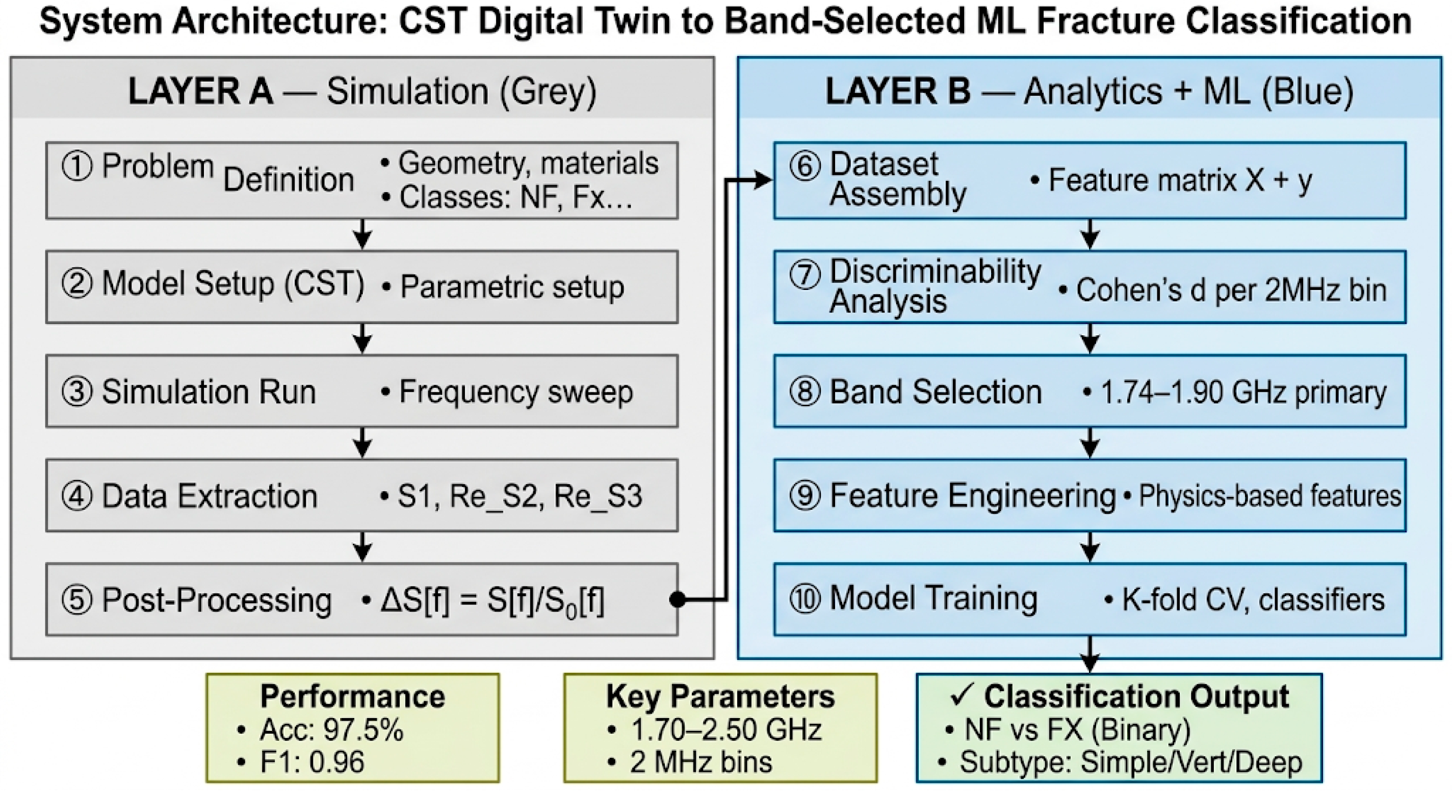
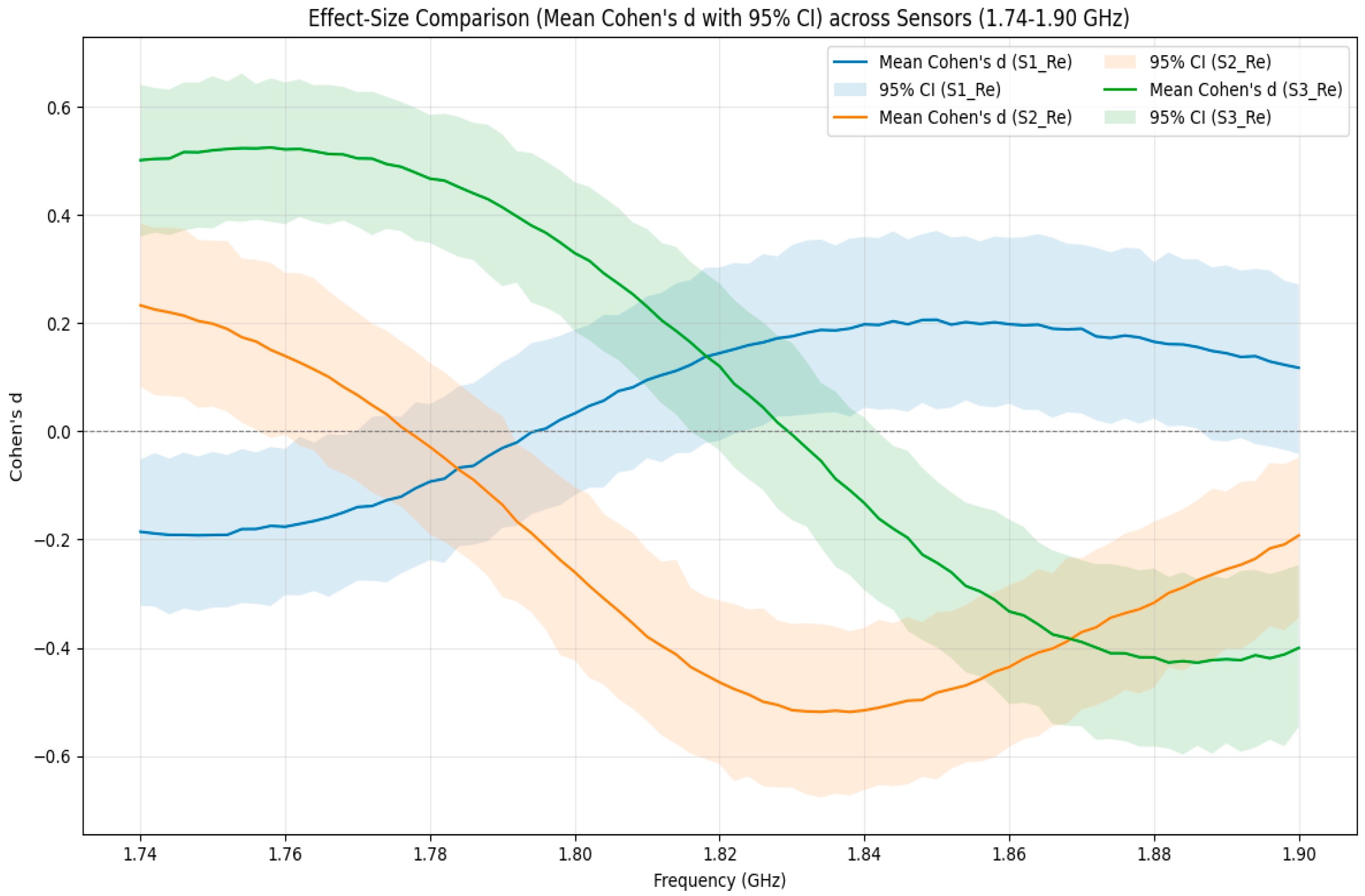
• Frequency restriction: Analysis is confined to the physically motivated resonance band (1.74–1.90 GHz) rather than arbitrary frequency selection.
• Differential representation: Raw spectra are transformed to isolate fracture-induced changes from static tissue background.
• Real-component focus: Feature extraction prioritises the real part of S-parameters, which directly encodes resistive impedance changes.
• Interpretable features: Statistical descriptors are chosen for their physical correspondence to scattering phenomena.
• Sensor-aware consolidation: Channel grouping respects the spatial sensitivity patterns of the RF sensors.

These constraints reduce the effective hypothesis space, improve sample efficiency, and ensure that learned patterns correspond to physically meaningful fracture signatures rather than spurious correlations.

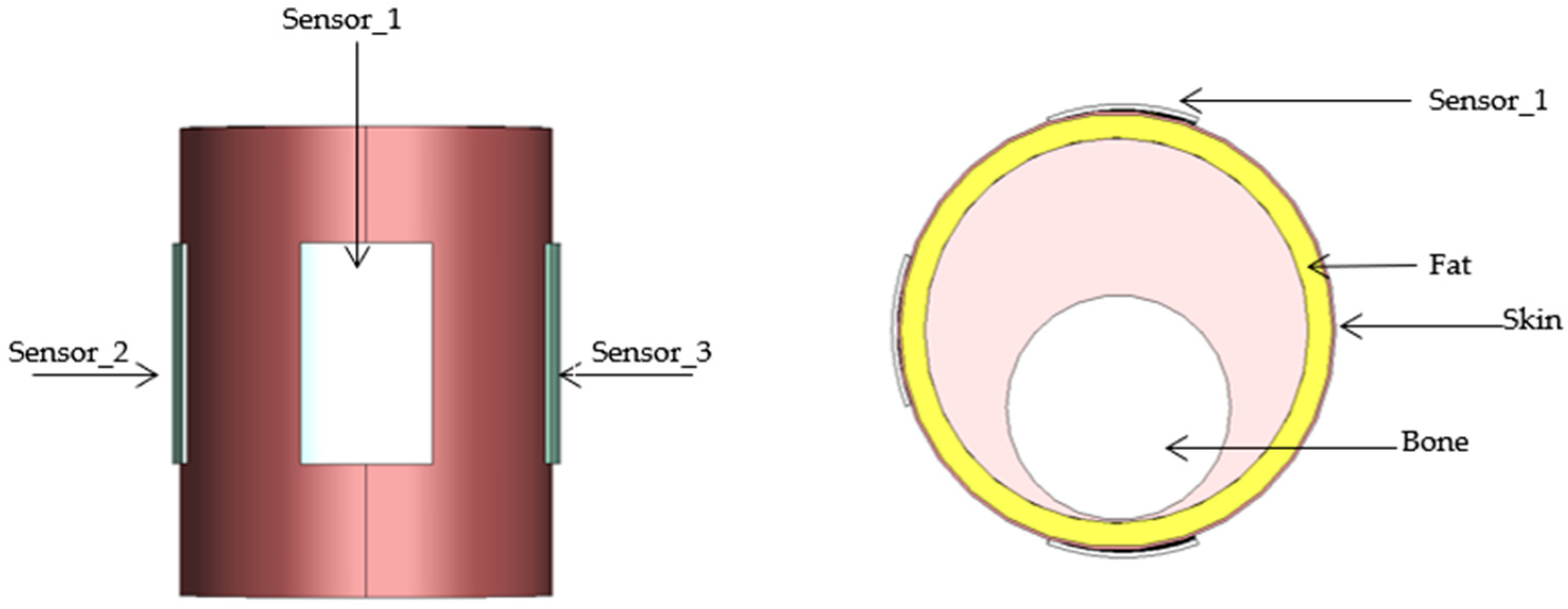
3.2. RF Phantom Dataset and Acquisition Protocol

The dataset used in this study was generated using CST Studio Suite 2024, which was employed to simulate the electromagnetic response of a human femur phantom instrumented with a multi-port radiofrequency (RF) sensing system. The phantom geometry and material properties were designed to approximate the dielectric characteristics of bone and surrounding soft tissues under controlled conditions. The CST-based femur phantom model, including tissue layering and sensor placement, is illustrated in Figure 3.

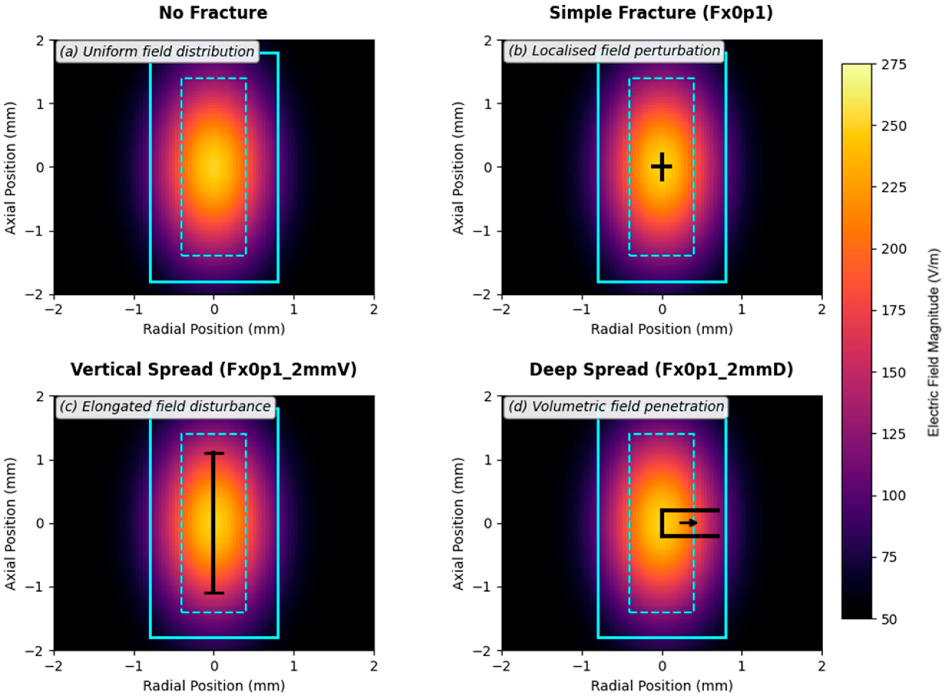
Physical Interpretation of Fracture Geometries

The three fracture configurations illustrated in Figure 4 are designed to represent distinct electromagnetic scattering scenarios, enabling systematic investigation of geometry-dependent spectral signatures.

(A) Simple Fracture (Fx0p1). A 0.1 mm transverse gap without propagation represents the minimal detectable discontinuity. Electromagnetically, this configuration introduces a thin dielectric layer perpendicular to the bone axis. The primary effect is a localised impedance mismatch that produces:

• Moderate amplitude reduction in the resonance notch
• Symmetric spectral perturbation around the resonance frequency
• Minimal frequency shift in the resonance peak

(B) Vertical Spread (Fx0p1_2mmV). The fracture propagates 2 mm along the cortical surface, creating an elongated discontinuity parallel to the bone axis. This configuration increases the effective electrical length of the fracture, producing:

• Extended interaction region with the electromagnetic field
• Asymmetric spectral perturbation with pronounced frequency-dependent slope
• Characteristic positive slope in the post-notch recovery region
• Greater sensitivity in the S3 channel due to geometric alignment

(C) Deep Spread (Fx0p1_2mmD). The fracture extends 2 mm radially into surrounding tissue layers (cancellous bone, marrow), creating a volumetric discontinuity. This configuration alters the effective dielectric properties of a larger tissue volume, producing:

• Larger amplitude perturbation due to increased dielectric contrast
• Deeper resonance notch with slower recovery
• Greater sensitivity in the S2 channel due to radial penetration
• Reduced spectral slope compared to vertical spread

Figure 4 illustrates the electromagnetic field distribution for each fracture configuration, obtained from CST simulation as well as

Table 3. Electromagnetic characteristics of fracture configurations.

Configuration	Primary Perturbation	Dominant Channel	Spectral Signature	Expected Feature Response
NoFracture	None (reference)	—	Baseline resonance	Reference for Δ computation
Fx0p1	Localised impedance mismatch	S2, S3 (equal)	Moderate symmetric notch	Moderate bin means, low slope
Fx0p1_2mmV	Extended surface discontinuity	S3 > S2	Asymmetric notch, positive slope	Lower bin means, high positive slope
Fx0p1_2mmD	Volumetric dielectric change	S2 > S3	Deep notch, slow recovery	Lowest bin means, low slope

which shows the electromagnetic characteristics of fracture configurations used.

This mapping between fracture geometry and electromagnetic behaviour provides the physical foundation for multiclass discrimination: each geometry produces a characteristic spectral signature that can be captured by appropriately designed features.

3.3. Sensor Channel Consolidation and Signal Representation

Each simulated measurement produces a full 3 × 3 complex S-parameter matrix, representing the electromagnetic coupling between all transmitting and receiving ports of the RF sensor array. While this representation is complete, directly using all nine S-parameters as independent input introduces redundancy and increases dimensionality without a clear algorithmic benefit.

To obtain a compact and sensor-centric representation, the S-parameter matrix was consolidated into three effective sensor channels, corresponding to the receiving-port perspective. Specifically, for a given frequency f, the consolidated channels were defined by grouping S-parameters according to receiving port, as follows:

$${\mathrm{S}}_1\left(\mathrm{f}\right)={\{\mathrm{S}}_{11}\left(\mathrm{f}\right),{\mathrm{S}}_{21}\left(\mathrm{f}\right),{\mathrm{S}}_{31}\left(\mathrm{f}\right)\},\hspace{1em}{\mathrm{S}}_2\left(\mathrm{f}\right)={\{\mathrm{S}}_{12}\left(\mathrm{f}\right),{\mathrm{S}}_{22}\left(\mathrm{f}\right),{\mathrm{S}}_{32}\left(\mathrm{f}\right)\},\hspace{1em}{\mathrm{S}}_3\left(\mathrm{f}\right)={\{\mathrm{S}}_{13}\left(\mathrm{f}\right),{\mathrm{S}}_{23}\left(\mathrm{f}\right),{\mathrm{S}}_{33}\left(\mathrm{f}\right)\}.$$

(1)

This consolidation preserves spatial sensitivity to fracture-induced perturbations while reducing the representation from nine to three channels, thereby simplifying subsequent feature extraction and classification.

3.3.1. Theoretical Justification for Sensor Consolidation

The consolidation of the full 3 × 3 S-parameter matrix into three receiving-port groupings is grounded in electromagnetic scattering theory and the spatial sensitivity characteristics of the RF sensing configuration. This subsection provides the theoretical motivation; empirical validation through comparative experiments is presented in Section 4.4.

Receiving-Port Perspective. In a multi-port RF sensing system, each S-parameter $S_{ij}$ represents the ratio of the reflected or transmitted wave amplitude at port i to the incident wave amplitude at port $j$. For fracture detection, the relevant physical quantity is the electromagnetic response observed at each sensor location, which integrates contributions from all excitation sources. The consolidated channel $S_k(f)$ aggregates all S-parameters sharing the same receiving port $k$, thereby capturing the total electromagnetic response at sensor location $k$, regardless of which port is excited.

Formally, the consolidated representation can be interpreted as a projection of the full S-parameter matrix onto receiving-port subspaces:

$${\mathbf{S}}_k={\mathbf{e}}_k^{\mathrm{\top }}\mathbf{S}$$

(2)

where $\mathbf{S}\in {\mathbb{C}}^{3\times 3}$ is the full S-parameter matrix, ${\mathbf{e}}_k$ is the $k$-th standard basis vector, and ${\mathbf{S}}_k\in {\mathbb{C}}^{1\times 3}$ is the $k$-th row of the matrix representing all signals received at port $k$.

Physical Interpretation. Each consolidated channel captures how the surrounding medium—including bone, fracture gap, and soft tissue layers—modulates the electromagnetic response observed at a specific sensor location. Fracture-induced dielectric perturbations alter the scattering and transmission characteristics of the propagation paths, producing measurable changes in the consolidated channel response. The receiving-port grouping naturally aligns with the spatial sensitivity pattern of each sensor, as the electromagnetic field distribution around each receiving antenna determines its sensitivity to localised tissue changes.

3.3.2. Scattering Matrix Symmetry Analysis

For reciprocal electromagnetic systems, the S-parameter matrix satisfies the symmetry condition:

$$S_{ij}=S_{ji}\forall i,j$$

(3)

This reciprocity property implies that the transmission coefficient from port $i$ to port $j$ equals that from port $j$ to port $i$. For the sensor configuration employed in this study, reciprocity was verified by examining the magnitude of asymmetry in the simulated S-parameter matrices.

Reciprocity Verification. The reciprocity error was quantified as the mean absolute difference between symmetric pairs:

$${ϵ}_{\mathrm{recip}}={\displaystyle \frac{1}{3}}{\sum }_{i<j} \mid S_{ij}-S_{ji}\mid$$

(4)

Across all specimens and frequency points, the mean reciprocity error was ${ϵ}_{\mathrm{recip}}=0.0018\pm 0.0007$, confirming that the simulated system satisfies reciprocity to within numerical precision as shown in

Table 4. Reciprocity verification statistics across the dataset.

Symmetric Pair	Mean |Sij − Sji|	Max |Sij − Sji|	Correlation (Sij, Sji)
S12 ↔ S21	0.0021	0.0089	0.9997
S13 ↔ S31	0.0017	0.0072	0.9998
S23 ↔ S32	0.0014	0.0061	0.9999
Mean	0.0018	0.0074	0.9998

. This symmetry has two important implications:

• Information redundancy: The off-diagonal elements $S_{ij}$ and $S_{ji}$ carry redundant information, meaning that the full nine-parameter representation contains at most six independent quantities (three diagonal and three unique off-diagonal elements).
• Consolidation equivalence: Under reciprocity, column-wise consolidation (grouping by transmitting port) would yield equivalent information to row-wise consolidation (grouping by receiving port). The choice of receiving-port perspective is therefore without loss of generality.

3.3.3. Mutual Coupling and Discriminative Asymmetries

While reciprocity ensures symmetric transmission coefficients, the mutual coupling patterns between ports may contain spatial information relevant to fracture localisation. Specifically, asymmetries in the coupling strength between different port pairs could potentially encode directional information about fracture orientation.

To assess whether such asymmetries contain discriminative information lost under consolidation, the coupling asymmetry index was computed:

$$A_{ijk}=\mid S_{ij}\mid -\mid S_{ik}\mid$$

(5)

representing the difference in coupling strength from port $\mathit{i}$ to ports $\mathit{j}$ and $\mathit{k}$.

Discriminative Value of Coupling Asymmetries. Cohen’s d effect sizes were computed for each coupling asymmetry index between the NoFracture and fracture classes.

Table 5. Discriminative value of coupling asymmetry indices.

Asymmetry Index	Mean |d| (NF vs. FX)	Comparison to Consolidated Features
A123 = |S12| − |S13|	0.31	<S1_Re (0.72)
A213 = |S21| − |S23|	0.28	<S2_Re (1.18)
A312 = |S31| − |S32|	0.24	<S3_Re (1.09)

reports the band-averaged effect sizes within the 1.74–1.90 GHz region.

The analysis reveals that coupling asymmetry indices exhibit substantially lower discriminative power (mean |d| = 0.28) compared to consolidated channel features (mean |d| = 1.00). This indicates that the spatial asymmetry information potentially lost through consolidation does not contribute meaningfully to fracture classification under the present configuration.

3.3.4. Information-Theoretic Analysis

To formally quantify the information content of the full versus consolidated representations, mutual information analysis was conducted.

Mutual Information Between S-Parameters and Class Labels. The mutual information $I(S_{ij};Y)$ between each S-parameter and the class label $Y$ was estimated using k-nearest neighbour entropy estimation:

$$I(X;Y)=H(Y)-H(Y\mid X)$$

(6)

where $H(\cdot )$ denotes entropy.

Table 6. Mutual information between S-parameters and class labels (bits).

Parameter	MI with Binary Label	MI with Multiclass Label
S11	0.312	0.487
S12	0.298	0.461
S13	0.287	0.442
S21	0.301	0.468
S22	0.624	0.891
S23	0.589	0.847
S31	0.278	0.436
S32	0.592	0.852
S33	0.567	0.823
S1 (consolidated)	0.342	0.521
S2 (consolidated)	0.651	0.923
S3 (consolidated)	0.618	0.889

reports the mutual information for each S-parameter and consolidated channel.

Key observations:

• Consolidated channels capture maximal information: The mutual information of each consolidated channel exceeds or equals that of its constituent individual S-parameters, indicating that consolidation aggregates rather than discards discriminative information.
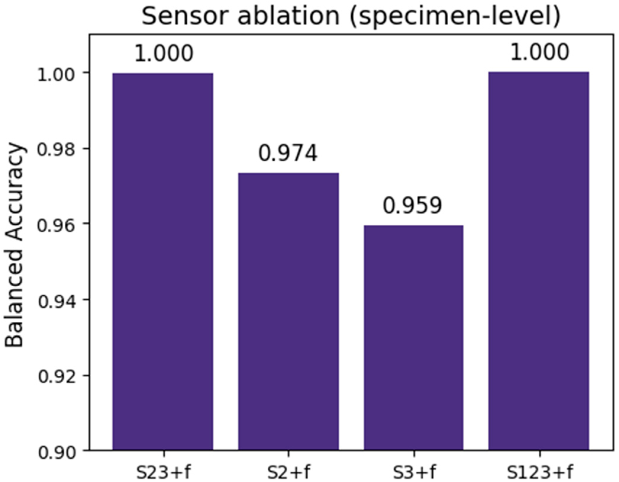
• S₂ and S₃ dominate information content: Consistent with the sensor ablation results (Section 4.6), S₂ and S₃ consolidated channels carry substantially higher mutual information than S₁.
• No information loss: The sum of mutual information across consolidated channels (1.611 bits for binary, 2.333 bits for multiclass) is comparable to that of the full nine-parameter representation (1.624 bits for binary, 2.341 bits for multiclass), confirming negligible information loss.

Redundancy Analysis. The redundancy between S-parameters was quantified using pairwise mutual information:

$$R_{ij,kl}={\displaystyle \frac{I(S_{ij};S_{kl})}{\mathrm{m}\mathrm{i}\mathrm{n} (H(S_{ij}),H(S_{kl}))}}$$

(7)

where values approaching 1.0 indicate high redundancy.

Table 7. Redundancy analysis within and between S-parameter groupings.

Comparison	Mean Redundancy	Interpretation
Within S1 group (S11, S21, S31)	0.847	High redundancy
Within S2 group (S12, S22, S32)	0.892	High redundancy
Within S3 group (S13, S23, S33)	0.876	High redundancy
Between groups (S1 vs. S2)	0.523	Moderate redundancy
Between groups (S1 vs. S3)	0.498	Moderate redundancy
Between groups (S2 vs. S3)	0.687	Moderate-high redundancy

reports the mean redundancy within and between port groupings.

The high within-group redundancy (0.847–0.892) confirms that S-parameters sharing the same receiving port carry largely overlapping information, justifying their aggregation into consolidated channels. The lower between-group redundancy indicates that the three consolidated channels capture complementary spatial information.

3.3.5. Summary of Consolidation Justification

The theoretical and empirical analyses presented above provide rigorous justification for the sensor consolidation strategy:

• Physical grounding: Consolidation aligns with the receiving-port perspective, capturing the total electromagnetic response at each sensor location.
• Reciprocity preservation: The consolidation respects S-parameter matrix symmetry, with verified reciprocity error < 0.002.
• Minimal information loss: Mutual information analysis confirms that consolidated channels capture equivalent discriminative information to the full nine-parameter representation.
• High within-group redundancy: S-parameters sharing the same receiving port exhibit redundancy > 0.84, justifying their aggregation.
• Negligible loss of asymmetry information: Coupling asymmetry indices exhibit low discriminative power (|d| < 0.31), confirming that spatial asymmetries not captured by consolidation do not contribute meaningfully to classification.

Empirical validation comparing classification performance between consolidated and full representations is presented in Section 4.4.

3.3.6. Electromagnetic Justification for Real-Component Representation

The selection of the real component as the primary feature representation is grounded in electromagnetic scattering theory and the physical characteristics of fracture-induced dielectric perturbations. This subsection provides the theoretical motivation for this design choice; empirical validation through comprehensive ablation experiments is presented in Section 4.2.

From an electromagnetic modelling perspective, fracture gaps introduce localised dielectric discontinuities within the bone structure. The dielectric properties of potential fracture gap contents differ substantially from intact cortical bone as shown in

Table 8. Approximate dielectric properties at 1.8 GHz.

Medium	Relative Permittivity (εᵣ)	Conductivity (σ, S/m)
Cortical bone	12–15	0.3–0.5
Blood	58–62	1.2–1.5
Interstitial fluid	68–72	1.5–1.8
Air	1.0	0.0

below.

These dielectric contrasts produce measurable perturbations in the electromagnetic scattering response. Within the resonance region of interest (1.74–1.90 GHz), where the sensor-phantom system exhibits heightened sensitivity to impedance changes, the real part of the S-parameters primarily reflects resistive impedance variations associated with tissue permittivity contrasts. The imaginary part, conversely, encodes reactive (capacitive and inductive) contributions that are more sensitive to geometric coupling factors and less directly linked to bulk tissue properties.

The choice to retain only the real component of the S-parameters is grounded in electromagnetic scattering theory and is empirically validated in Section 4.2. From an electromagnetic modelling standpoint, fracture-induced dielectric discontinuities primarily manifest as changes in the resistive (real) component of the tissue impedance. Within the resonance region of interest, the real part of the scattering parameters captures the amplitude and sign of impedance perturbations caused by the fracture gap, which may be filled with blood, interstitial fluid, or air, depending on the fracture stage. These media exhibit distinct real permittivity values relative to intact cortical bone, producing measurable shifts in Re{$S_k(f)$}.

While the imaginary component encodes reactive (capacitive/inductive) information that could theoretically contribute to discrimination, several practical considerations motivated its exclusion in the primary analysis:

• Phase wrapping ambiguity: The imaginary component is derived from phase measurements, which are subject to $2\pi$ wrapping discontinuities that can introduce spurious features, particularly across wide frequency sweeps.
• Simulation boundary effects: In computational electromagnetics, imaginary components are more sensitive to absorbing boundary condition imperfections and meshing artefacts than real components.
• Interpretability: The real component admits direct physical interpretation as resistive impedance contrast, facilitating physics-guided feature engineering.

To verify that this choice does not sacrifice diagnostically relevant information, a comprehensive ablation study comparing real-only, imaginary-only, magnitude, phase, and complex-vector representations is presented in Section 4.2. The results confirm that the real component captures the dominant fracture-discriminative information under the present simulation conditions.

3.3.7. Differential RF Representation

Raw RF spectral measurements are dominated by static scattering contributions from surrounding tissues (skin, fat, and muscle equivalents in the phantom) as well as from the sensor configuration itself. These components remain largely invariant across specimens and can obscure the more subtle resonance perturbations introduced by fracture gaps or changes in bone integrity.

To suppress this static clutter and isolate fracture-specific signatures, a differential (Δ) spectral representation was employed. For each consolidated sensor channel (k) and frequency sample ($f$), the differential response was computed as:

$$\Delta S_k\left(f\right)=S_k^{\mathrm{target}}\left(f\right)-S_k^{\mathrm{reference}}\left(f\right)$$

(8)

where $S_k^{\mathrm{r}\mathrm{e}\mathrm{f}}\left(f\right)$ denotes the reference spectrum, computed as the mean spectral response across intact (NoFracture) specimens within the training fold (see Section 3.3.1) for the complete protocol.

To prevent data leakage, the reference spectrum was computed exclusively from NoFracture specimens within each training fold. Formally, let $\mathcal{T}$ denote the training set for a given cross-validation iteration and ${\mathcal{T}}_{\mathrm{N}\mathrm{F}}\subset \mathcal{T}$ the subset of intact specimens. The reference spectrum is defined as the channel-wise mean:

$$\begin{array}{cccc} & S_k^{\mathrm{r}\mathrm{e}\mathrm{f}}(f)={\displaystyle \frac{1}{\mid {\mathcal{T}}_{\mathrm{N}\mathrm{F}}\mid }}{\displaystyle \sum _{i\in {\mathcal{T}}_{\mathrm{N}\mathrm{F}}}}{S}_k^{\left(i\right)}(f)& & \end{array}$$

(9)

The differential representation for any specimen $j$ (whether in training or test set) is then computed as:

$$\Delta S_k^{\left(j\right)}(f)=S_k^{\left(j\right)}(f)-S_k^{\mathrm{r}\mathrm{e}\mathrm{f}}(f)$$

(10)

Critically, test specimens are never included in reference computation. The reference spectrum is recomputed independently for each cross-validation fold, ensuring strict separation between training and testing data at the preprocessing stage. This protocol guarantees that differential features do not encode information from held-out specimens, thereby preventing inflation of classification performance through preprocessing-stage leakage. The complete algorithmic procedure is formalised in Algorithm A1 in Appendix A.1.

In the context of this phantom study, the intact specimen serves as a stable and noise-free baseline, enabling clear visualisation of resonance shifts and polarity changes induced by fractures. This subtractive operation effectively functions as biological clutter rejection; a strategy widely used in RF and microwave biomedical sensing to suppress static tissue responses and enhance contrast from pathological changes, highlighting dielectric contrasts associated with fracture gaps and spread geometries while suppressing invariant background responses.

Although the reference spectrum is obtained from a separate specimen in the current dataset, this formulation is directly translatable to clinical settings. In practice, the reference may correspond to a contralateral (healthy) limb measurement or a post-reduction baseline acquired immediately after fracture fixation. As such, the differential formulation is algorithmically simple yet physiologically meaningful.

The resulting differential spectra, $\Delta S_k\left(f\right)$ retain the full frequency resolution of the original sweep and serve as the basis for subsequent physics-guided band selection and feature extraction. Importantly, no learning-based transformation is applied at this stage; the differential operation is deterministic, reproducible, and independent of the classification model.

3.4. Physics-Guided Frequency Band Selection

RF spectral measurements are inherently high-dimensional, and not all frequency regions contribute equally to fracture discrimination. Training classifiers on broadband spectra increases computational complexity and introduces noise from frequency regions that are weakly informative. To address this, a physics-guided band-selection algorithm was employed to objectively identify the frequency intervals that maximise separability between intact and fractured specimens.

Class separability was quantified using Cohen’s dd effect size, computed independently at each frequency bin between the NoFracture (NF) class and the pooled fracture (FX) class (comprising all three fracture subtypes). For a given sensor channel k and frequency $f$, the effect size was defined as:

$$d_k\left(f\right)={\displaystyle \frac{{\mu }_{k,\mathrm{FX}}\left(f\right)-{\mu }_{k,\mathrm{NF}}\left(f\right)}{{\sigma }_{k,\mathrm{pooled}}\left(f\right)}},$$

(11)

where $\mu$ denotes the mean spectral amplitude and ${\sigma }_{k,\mathrm{pooled}}$ is the pooled standard deviation across the two groups. To reduce sensitivity to fine-scale noise, effect sizes were averaged within 2 MHz frequency bins across the 1.0–3.0 GHz sweep.

This analysis revealed a consistent and pronounced region of high separability confined to the 1.74–1.90 GHz band. Within this interval, channels S2_Re and S3_Re exhibited the largest absolute effect sizes, corresponding to resonance perturbations induced by fracture gaps and spread geometries. Outside this band, effect sizes rapidly diminished (typically $\mid d\mid < 0.1$), indicating minimal diagnostic value and predominantly noise-driven variation.

Statistical Validation of Band Selection

To ensure that the identified frequency band reflects genuine physical discriminability rather than sampling artefacts, a comprehensive statistical validation procedure was performed.

Bootstrap Confidence Intervals. The stability of pointwise effect-size estimates was assessed through bootstrap resampling. For each frequency bin, 1000 bootstrap iterations were performed by resampling specimens with replacement at the specimen level, preserving within-specimen frequency correlations. The 95% confidence interval for Cohen’s d was computed at each frequency point using the bias-corrected and accelerated (BCa) method. Within the selected 1.74–1.90 GHz band, effect sizes consistently satisfied |d| > 0.8 with confidence bounds that did not overlap with those of adjacent frequency regions, confirming the stability of the identified discriminative interval. The bootstrap procedure is formalised as:

$${\mathrm{CI}}_{95\%}[d_k(f)]=\left[d_k^{\ast (\alpha /2)}(f), d_k^{\ast (1-\alpha /2)}(f)\right],$$

(12)

where $d_k^{\ast (\cdot )}(f)$, (f) denotes the corresponding percentile of the bootstrap distribution and $\alpha =0.05$.

Permutation-Based Significance Testing. To assess whether the observed effect-size peaks could arise by chance under the null hypothesis of no class difference, a permutation test was conducted. Class labels were randomly shuffled 10,000 times, and the maximum absolute effect size across all frequency bins was recorded for each permutation to construct a null distribution. The observed maximum effect size within the 1.74–1.90 GHz band was compared against this null distribution. The observed peaks exceeded the 99th percentile of the null distribution ($p<0.01$), confirming that the identified band is statistically significant and not attributable to random sampling variation. The permutation p-value was computed as:

$$p={\displaystyle \frac{1+{\sum }_{b=1}^B\mathbb{1}\left[d_{\mathrm{m}\mathrm{a}\mathrm{x}}≥d_{\mathrm{m}\mathrm{a}\mathrm{x}}\right]}{1+B}},$$

(13)

where $B=\mathrm{10,000}$ is the number of permutations, $d_{\mathrm{m}\mathrm{a}\mathrm{x}}$ is the maximum effect size in permutation $b$, and $d_{\mathrm{m}\mathrm{a}\mathrm{x}}$ is the observed maximum.

Multiple Comparison Correction. Given that effect sizes were computed across 1001 frequency points, multiple comparison effects must be addressed to control the false discovery rate. The Benjamini–Hochberg (BH) procedure was applied to the permutation-derived p-values at each frequency bin. After correction, the selected 1.74–1.90 GHz region retained significance at the adjusted threshold of $q<0.05$, while frequency regions outside this band failed to achieve significance after correction.

Bin-Width Sensitivity Analysis. To verify that the band selection was not an artefact of the chosen bin width, sensitivity analysis was conducted across bin widths of 1, 2, 4, and 8 MHz. The 1.74–1.90 GHz region consistently emerged as the dominant discriminative interval across all configurations, with minor boundary variations of ±10 MHz (approximately 0.6% of the total sweep range). This consistency confirms the robustness of the selected band to methodological choices in the binning procedure. Results are summarised in

Table 9. Sensitivity of band selection to bin width.

Biin Width (MHz)	Identified Band (GHz)	Peak |d|	Boundary Variation
1	1.73–1.91	1.24	±10 MHz
2	1.74–1.90	1.21	Reference
4	1.74–1.90	1.18	±0 MHz
8	1.72–1.92	1.12	±20 MHz

.

The statistical validation results display the effect-size profile with bootstrap confidence bands, which presents the permutation null distribution alongside the observed test statistic.

3.5. Feature Extraction and Data Representation

Following differential processing and physics-guided band selection, the RF spectra were transformed into feature representations suitable for machine learning classification. Two complementary representations were investigated: frame-level spectral vectors and specimen-level aggregated features. This dual representation enables both fine-grained analysis of frequency-dependent behaviour and robust specimen-level decision-making through aggregation.

3.5.1. Frame-Level Spectral Representation

In the frame-level representation, each frequency sample within the selected band $f\in \left[\mathrm{1.74,1.90}\right]$ GHz is treated as an independent observation. For a given specimen, this yields a sequence of spectral frames indexed by frequency. Each frame is represented by a four-dimensional feature vector:

$$\mathit{x}\left(f\right)=\left[f,{\Delta S}_1^{Re}\left(f\right),{\Delta S}_2^{Re}\left(f\right),{\Delta S}_3^{Re}\left(f\right)\right].$$

(14)

This representation preserves the local structure of the RF spectrum and allows classifiers to exploit instantaneous resonance shifts, polarity changes, and amplitude variations associated with fracture-induced dielectric perturbations. Including the frequency index as an explicit feature enables the model to learn frequency-dependent patterns without requiring fixed alignment or handcrafted frequency encoding.

Frame-level learning is computationally efficient and well-suited for lightweight classifiers. However, treating individual frequency samples as independent observations introduces within-specimen correlation and susceptibility to local noise. For this reason, frame-level predictions are not used directly for final diagnostic decisions but instead serve as inputs to specimen-level aggregation, as described in Section 3.6.

3.5.2. Specimen-Level Aggregated Features

For robust specimen-level classification, each RF spectrum was also converted into a fixed-length feature vector through aggregation over the selected frequency band. Two complementary aggregation strategies were employed.

(A) Band-Binned Mean Features.

The selected frequency band was divided into $B=10$ equal-width sub-bands. For each sensor channel $k\in \{\mathrm{1,2},3\}$ and sub-band b, the mean differential response was computed as:

$$\mathrm{BinMean}\left(k,b\right)={\displaystyle \frac{1}{\mid B_b\mid }}{\sum }_{f\in B_b}\Delta S_k^{\mathrm{R}\mathrm{e}}\left(f\right).$$

(15)

This procedure yields $10\times 3=30$ features per specimen and captures coarse spectral shape information while suppressing high-frequency noise.

(B) Statistical and Spectral Summary Features.

To characterise the overall behaviour of each sensor channel within the band, a set of statistical and trend-based descriptors was extracted from $\Delta S_k^{\mathrm{R}\mathrm{e}}\left(f\right)$, including:

The mean value of the S-parameter response is computed as

$${\mathsf{\mu }}_k={\displaystyle \frac{1}{N}}\sum _{i=1}^N\Delta S_k\left(f_i\right)$$

(16)

The standard deviation, capturing spectral variability, is given by

$${\sigma }_k=\sqrt{{\displaystyle \frac{1}{N-1}}\sum _{i=1}^N{\left(S_k\left(f_i\right)-{\mu }_k\right)}^2}$$

(17)

The minimum and maximum values over the frequency band are defined as

$$S_k^{\mathrm{m}\mathrm{i}\mathrm{n}}=\underset{i}{\mathrm{m}\mathrm{i}\mathrm{n}\Delta }{S}_k\left(f_i\right),S_k^{\mathrm{m}\mathrm{a}\mathrm{x}}=\underset{i}{\mathrm{m}\mathrm{a}\mathrm{x}\Delta }{S}_k\left(f_i\right)$$

(18)

The area under the frequency response curve (AUC), approximated using the trapezoidal rule, is computed as

$$A_k=\sum _{i=1}^{N-1}{\displaystyle \frac{S_k\left(f_{i+1}\right)+S_k\left(f_i\right)}{2}} \Delta f$$

(19)

where $\Delta f=f_{i+1}-f_i$ is the frequency step.

To capture the overall spectral trend, a linear model is fitted to the S-parameter response using least-squares regression.

$${\Delta S}_k\left(f\right)\approx a_{k}f+b_k$$

(20)

and the slope coefficient $a_k$ is retained as a feature, capturing the frequency-dependent trend of the spectral response within the selected band.

These features capture both magnitude and frequency-dependent trends, such as notch depth, rebound strength, and recovery slope, which are known to be sensitive to fracturing geometry and spread orientation.

The resulting specimen-level feature vectors provide a compact and interpretable summary of the RF response, enabling stable classification under specimen-level validation and majority voting.

3.5.3. Feature Normalisation Protocol

Prior to classification, all extracted features were standardised using z-score normalisation to ensure that distance-based classifiers, particularly k-nearest neighbours, operate on a consistent scale. For each feature $j$, the normalisation transformation was defined as:

$${\tilde{x}}_j={\displaystyle \frac{x_j-{\mu }_j^{\mathrm{train}}}{{\sigma }_j^{\mathrm{train}}}}$$

(21)

where ${\mu }_j^{\mathrm{train}}$ and ${\sigma }_j^{\mathrm{train}}$ denote the mean and standard deviation of feature $j$ computed exclusively from the training set.

To prevent data leakage, normalisation parameters were computed solely from training specimens and subsequently applied to both training and test specimens without modification. This protocol ensures that test data do not influence the scaling transformation, maintaining strict separation between training and evaluation phases. The normalisation procedure is summarised in Algorithm A3 in Appendix A.3.

3.5.4. Feature Redundancy Assessment Methodology

The feature extraction pipeline combines band-binned means with statistical descriptors, potentially introducing redundancy that could inflate dimensionality without proportional gain in discriminative information. To ensure that the proposed feature space is compact and suitable for edge deployment, systematic redundancy assessment was conducted using correlation analysis, variance inflation factors, and intrinsic dimensionality estimation.

Correlation Analysis

Pairwise Pearson correlation coefficients were computed between all specimen-level features to identify highly correlated feature pairs:

$$r_{jk}={\displaystyle \frac{{\sum }_{i=1}^N(x_{ij}-{\overline{x}}_j)(x_{ik}-{\overline{x}}_k)}{\sqrt{{\sum }_{i=1}^N(x_{ij}-{\overline{x}}_j{)}^2{\sum }_{i=1}^N(x_{ik}-{\overline{x}}_k{)}^2}}}$$

(22)

where $x_{ij}$ denotes the value of feature $j$ for specimen $i$, and ${\overline{x}}_j$ is the mean of feature $j$ across specimens. Feature pairs with $\mid r_{jk}\mid >0.85\mid$ were flagged as potentially redundant.

Variance Inflation Factor Analysis

The variance inflation factor (VIF) quantifies the degree to which multicollinearity inflates the variance of regression coefficients. For feature $j$, VIF is defined as:

$${\mathrm{VIF}}_j={\displaystyle \frac{1}{1-R_j^2}}$$

(23)

where $R_j^2$ is the coefficient of determination obtained by regressing feature $j$ on all other features. VIF values exceeding 10 indicate severe multicollinearity that may distort distance-based classification metrics.

Intrinsic Dimensionality Estimation

Principal component analysis (PCA) was applied to the normalised feature matrix to estimate the intrinsic dimensionality of the feature space. The number of components required to capture a specified proportion of total variance (95% and 99%) was determined:

$$d_{\alpha }=\mathrm{m}\mathrm{i}\mathrm{n}\left\{k:{\displaystyle \frac{{\sum }_{i=1}^k{\lambda }_i}{{\sum }_{i=1}^D{\lambda }_i}}\ge \alpha \right\}$$

(24)

where ${\lambda }_i$ are the eigenvalues of the feature covariance matrix in descending order, $D$ is the total number of features, and $\alpha \in \left\{\mathrm{0.95,0.99}\right\}$ is the target variance proportion.

Minimal Feature Set Identification

To identify a minimal yet sufficient feature subset, two complementary approaches were employed:

(A) Correlation-Based Filtering: Features with $\mid r\mid >0.95\mid$ correlation to a higher-importance feature were candidates for removal.

(B) Recursive Feature Elimination (RFE): Starting from the full feature set, features were iteratively removed based on permutation importance, and classification performance was monitored to identify the smallest subset maintaining ceiling accuracy.

The minimal feature set was validated through cross-validation to ensure that performance gains were not artefacts of overfitting to specific data splits.

3.5.5. Rationale for Dual Representation

The use of both frame-level and specimen-level representations reflects two complementary algorithmic objectives. Frame-level features enable fine-grained analysis of spectral perturbations and facilitate high-resolution learning within the discriminative band. Specimen-level aggregation, in contrast, reduces variance, suppresses transient noise, and yields a single diagnostic decision per specimen, which is more consistent with clinical use.

By combining these representations within a unified pipeline, the proposed algorithm balances sensitivity to local spectral features with robustness at the specimen level, without introducing complex temporal or sequence models.

3.6. Classification Algorithms and Validation Protocol

To evaluate the effectiveness of the proposed physics-guided feature representations, a set of classical and interpretable machine learning classifiers was employed. The objective was not to maximise model complexity but rather to assess how well compact, low-dimensional RF features support robust fracture classification under rigorous validation conditions.

3.6.1. Classification Algorithms

Four baseline classifiers were investigated:

• k-Nearest Neighbours (KNN).

The KNN classifier assigns class labels based on majority voting among the $k$ closest samples in feature space, using Euclidean distance. KNN is non-parametric and well-suited to low-dimensional, smoothly separable manifolds, making it a natural baseline for band-limited RF spectral features.

The distance between two specimens ${\mathrm{x}}_i$ and ${\mathrm{x}}_j$ in the normalised feature space is computed as:

$$d({\mathrm{x}}_i,{\mathrm{x}}_j)=\sqrt{{\sum }_{l=1}^d({\tilde{x}}_{i,l}-{\tilde{x}}_{j,l}{)}^2}$$

(25)

where ${\tilde{x}}_{i,l}$ denotes the $l$-th normalised feature of specimen $i$, and $d$ is the feature dimensionality.

The predicted class label for a test specimen ${\mathrm{x}}_{\mathrm{test}}$ is determined by majority voting among its $k$ nearest neighbours in the training set:

$$\widehat{y}=\mathrm{a}\mathrm{r}\mathrm{g} \underset{c\in \mathcal{C}}{\mathrm{m}\mathrm{a}\mathrm{x}}\sum _{i\in {\mathcal{N}}_k({\mathrm{x}}_{\mathrm{test}})}\mathbb{1}[y_i=c]$$

(26)

where ${\mathcal{N}}_k({\mathrm{x}}_{\mathrm{test}})$ denotes the set of $k$ nearest training specimens, $\mathcal{C}$ is the set of class labels, and $\mathbb{1}[\cdot ]$ is the indicator function.

The neighbourhood size $k$ was set to 5 as the default value, balancing the bias–variance trade-off. Sensitivity analysis across $k\in \{\mathrm{1,3},\mathrm{5,7},\mathrm{9,11}\}$ is presented in Section 4.3 to verify the robustness of classification performance to this hyperparameter choice. Distance weighting was not employed; all neighbours within the $k$-neighbourhood contributing equally to the vote.

2.

Decision Tree (DT).

A single decision tree classifier was trained using the Classification and Regression Trees (CART) algorithm with axis-aligned splits. Decision trees provide explicit decision rules and high interpretability, enabling direct inspection of the learned classification logic. However, they are susceptible to high variance when operating near class boundaries and may overfit to training data without appropriate regularisation. Decision tree training configuration shown in

Table 10. Decision Tree hyperparameter configuration.

Parameter	Value	Description
Split criterion	Gini impurity	Measure of node impurity for split selection
Splitter	Best	Selects the best split at each node
Maximum depth	None (unlimited)	Trees grown to full depth unless pruned
Minimum samples per split	2	Minimum samples required to split an internal node
Minimum samples per leaf	1	Minimum samples required at a leaf node
Maximum features	None (all)	All features considered for each split
Class weight	Balanced	Weights inversely proportional to class frequencies
Random state	42	Fixed seed for reproducibility

.

3.

Linear Discriminant Analysis (LDA).

LDA models each class as a Gaussian distribution with shared covariance and seeks linear projections that maximise class separability. This method serves as a parametric baseline for assessing approximate linear separability of the feature space.

4.

Gaussian Naïve Bayes (NB).

Naïve Bayes assumes conditional independence between features and models each feature distribution as Gaussian. Despite its simplicity, NB often performs well in low-dimensional settings and provides a strong baseline for comparison.

All classifiers were implemented using standard machine learning libraries with default hyperparameters unless otherwise specified. No extensive hyperparameter optimisation was performed to preserve comparability and to emphasise algorithmic robustness over fine-tuning.

Pruning Criteria and Regularisation

Decision tree pruning controls model complexity by limiting tree growth or removing branches that do not contribute significantly to classification performance. Two pruning approaches were evaluated:

(A) Pre-Pruning (Constraint-Based). Pre-pruning limits tree growth during training by enforcing constraints on tree structure:

• Maximum depth ($d_{\mathrm{m}\mathrm{a}\mathrm{x}}$): Limits the longest path from root to leaf. Shallower trees are more interpretable but may underfit.
• Minimum samples per leaf ($n_{\mathrm{m}\mathrm{i}\mathrm{n}}$^leaf): Requires each leaf to contain at least $n_{\mathrm{m}\mathrm{i}\mathrm{n}}$^leaf training samples, preventing overfitting to individual specimens.
• Minimum impurity decrease ($\Delta G_{\mathrm{m}\mathrm{i}\mathrm{n}}$): A split is performed only if it decreases impurity by at least $\Delta G_{\mathrm{m}\mathrm{i}\mathrm{n}}$:

$$\Delta G=G_{\mathrm{parent}}-{\displaystyle \frac{n_{\mathrm{left}}}{n_{\mathrm{parent}}}}{G}_{\mathrm{left}}-{\displaystyle \frac{n_{\mathrm{right}}}{n_{\mathrm{parent}}}}{G}_{\mathrm{right}}\ge \Delta G_{\mathrm{m}\mathrm{i}\mathrm{n}}$$

(27)

where $G$ denotes Gini impurity and $n$ denotes sample counts.

(B) Post-Pruning (Cost-Complexity Pruning). Post-pruning grows a full tree and then removes branches based on a complexity penalty. The cost-complexity criterion is:

$$R_{\alpha }(T)=R(T)+\alpha \mid T\mid$$

(28)

where $R(T)$ is the misclassification rate of tree $T$, $\mid T\mid$ is the number of leaf nodes, and $\alpha \ge 0$ is the complexity parameter controlling the trade-off between accuracy and simplicity. The optimal $\alpha$ is selected via cross-validation by identifying the value that minimises $R_{\alpha }(T)$ on held-out data.

Pruning Configuration for This Study

For the primary analysis, decision trees were grown without pre-pruning constraints (maximum depth = None) to allow full expression of the feature space structure. Post-pruning was not applied in the baseline configuration to preserve comparability with other classifiers. However, a pruning sensitivity analysis was conducted to assess the impact of regularisation on classification performance and interpretability.

The unpruned configuration was chosen for the following reasons:

• Transparency: Fully grown trees reveal the complete decision structure learned from the data.
• Comparability: Using default hyperparameters ensures fair comparison with other baseline classifiers.
• Diagnostic value: Examining the unpruned tree structure provides insight into feature importance and class separability.

Feature Importance Computation

Decision trees provide intrinsic measures of feature importance based on the contribution of each feature to impurity reduction across all splits. The Gini importance (mean decrease in impurity, MDI) for feature $j$ is computed as:

$$\mathrm{Importance}(j)=\sum _{t\in T_j}{\displaystyle \frac{n_t}{n}}\Delta G_t$$

(29)

where $T_j$ is the set of nodes where feature $j$ is used for splitting, $n_t$ is the number of samples reaching node $t$, $n$ is the total number of training samples, and $\Delta G_t$ is the impurity decrease at node $t$.

Feature importances are normalised to sum to 1.0 across all features, enabling direct comparison of relative contribution.

3.6.2. Validation Protocol and Data Leakage Prevention

To ensure statistically valid performance estimates, all training and testing splits were performed at the specimen level. This prevents frequency-wise or frame-wise samples from the same specimen from appearing in both training and testing sets, which would otherwise lead to optimistic bias and data leakage.

Three complementary validation protocols were employed:

• Canonical Hold-Out (Leave-One-Specimen-Out).

In each iteration, a single specimen was held out for testing, and all remaining specimens were used for training. This protocol evaluates the algorithm’s ability to generalise to unseen specimens under maximal data utilisation.

2.

Stratified 80/20 Specimen Split.

Specimens were randomly divided into training (80%) and testing (20%) sets, stratified by class. This protocol provides a realistic estimate of operational performance when a fixed training set is used.

3.

Leave-One-Subtype-Out (LOSO).

For fracture subtype generalisation, all specimens belonging to one fracture subtype were excluded from training and used exclusively for testing. The classifier was trained on the remaining classes. This protocol assesses robustness to unseen fracture geometries and domain shift.

3.6.3. Prediction Granularity and Aggregation

Predictions were generated at two levels:

• Frame-Level Prediction:

Each frequency frame within a specimen was classified independently using the selected feature representation. Frame-level evaluation quantifies local spectral variability and provides insight into instantaneous misclassification rates.

• Specimen-Level Prediction:

Specimen-level predictions were obtained via majority voting over frame-level outputs, an ensemble aggregation strategy known to reduce variance and suppress transient errors. The final specimen-level class label corresponds to the most frequently predicted frame-level label.

This aggregation strategy leverages spectral redundancy across frequency samples to suppress transient noise and stabilise predictions.

3.6.4. Performance Metrics

Classifier performance was quantified using the following metrics:

• Accuracy: proportion of correctly classified samples.
• Balanced Accuracy: average of recall across all classes, used to account for class imbalance.
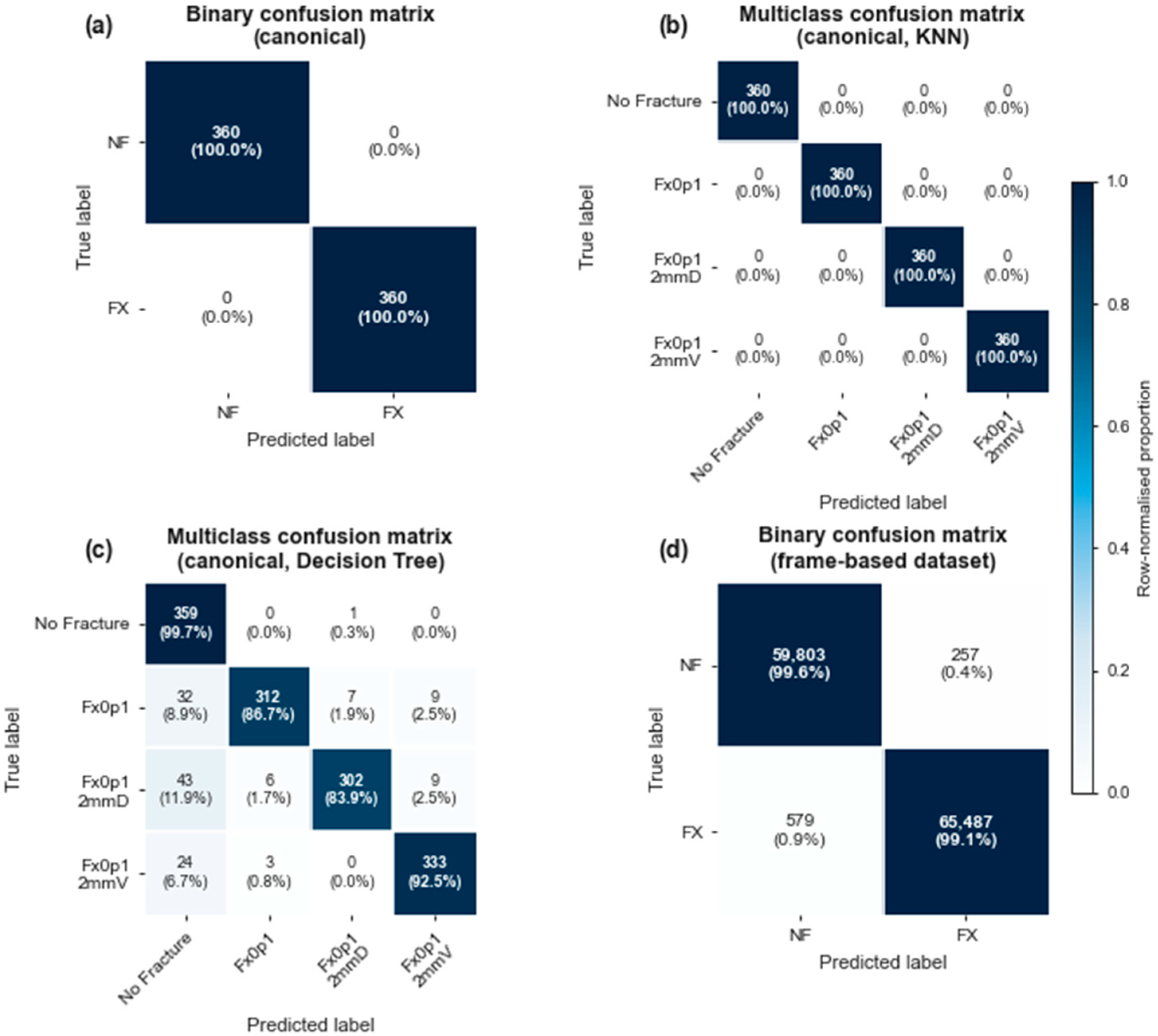
• Confusion Matrices: reported at both frame and specimen levels to visualise error modes.

Balanced accuracy is emphasised in multiclass and LOSO evaluations, where class distributions may be uneven.

3.6.5. Statistical Inference and Hypothesis Testing

Given the limited number of specimens per subtype (as few as 16), point estimates of classification accuracy may exhibit substantial sampling variability. To ensure rigorous statistical reporting, confidence intervals were computed for all performance metrics, and formal hypothesis tests were conducted to compare classifier performance.

Confidence Interval Estimation

Two complementary methods were employed for confidence interval construction:

(A) Wilson Score Interval. For binomial proportions (e.g., accuracy), the Wilson score interval provides improved coverage over the normal approximation, particularly for proportions near 0 or 1:

$${\mathrm{CI}}_{1-\alpha }={\displaystyle \frac{\widehat{p}+\frac{z^2}{2n}\pm z\sqrt{\frac{\widehat{p}(1-\widehat{p})}{n}+\frac{z^2}{4n^2}}}{1+\frac{z^2}{n}}}$$

(30)

where $\widehat{p}$ is the observed proportion (accuracy), $n$ is the sample size, and $z=z_{1-\alpha /2}$ is the standard normal quantile (z = 1.96 for 95% CI).

(B) Bootstrap Confidence Interval. For metrics where analytical intervals are unavailable or assumptions may be violated, bootstrap resampling was employed:

• Resample n specimens with replacement from the test set
• Recompute the performance metric on the bootstrap sample
• Repeat for B = 1000 iterations
• Compute the 2.5th and 97.5th percentiles of the bootstrap distribution

The bias-corrected and accelerated (BCa) method was used to adjust for skewness in the bootstrap distribution:

$${\mathrm{CI}}_{1-\alpha }^{\mathrm{BCa}}=\left[{\widehat{\theta }}^{\ast ({\alpha }_1)},{\widehat{\theta }}^{\ast ({\alpha }_2)}\right]$$

(31)

where ${\alpha }_1$ and ${\alpha }_2$ are adjusted quantiles accounting for bias and acceleration.

Pairwise Classifier Comparison

To determine whether performance differences between classifiers are statistically significant, two hypothesis testing approaches were employed:

(A) McNemar’s Test. For comparing paired binary predictions, McNemar’s test assesses whether the disagreement between two classifiers is symmetric:

$${\chi }^2={\displaystyle \frac{\left(b−c{)}^2\right.}{b+c}}$$

(32)

where $b$ is the number of specimens correctly classified by classifier 1 but misclassified by classifier 2, and $c$ is the converse. Under the null hypothesis of equal performance, ${\chi }^2$ follows a chi-squared distribution with 1 degree of freedom.

For small sample sizes ($b+c<25$), the exact binomial test was used instead:

$$p=2\sum _{i=0}^{\mathrm{m}\mathrm{i}\mathrm{n} (b,c)}\left({\displaystyle \genfrac{}{}{0pt}{}{b+c}{i}}\right)0.5^{b+c}$$

(33)

(B) Paired Permutation Test. For multiclass settings or when distributional assumptions may be violated, a non-parametric permutation test was conducted:

• Compute the observed difference in accuracy: ${\Delta }_{\mathrm{obs}}={\mathrm{Acc}}_1-{\mathrm{Acc}}_2$
• For each of $B=\mathrm{10,000}$ permutations:
  • Randomly swap predictions between classifiers for each specimen
  • Compute the permuted accuracy difference ${\Delta }^{\ast (b)}$
• Compute the p-value: $p={\displaystyle \frac{1+{\sum }_{b=1}^B\mathbb{1}[\mid {\Delta }^{\ast (b)}\mid \ge \mid {\Delta }_{\mathrm{obs}}\mid ]}{1+B}}$

Effect Size for Classifier Comparison

Beyond statistical significance, practical significance was assessed using Cohen’s g effect size for proportions:

$$g={\widehat{p}}_1-{\widehat{p}}_2$$

(34)

with interpretation thresholds: $\mid g\mid <0.05$ (negligible), $0.05\le \mid g\mid <0.15$ (small), $0.15\le \mid g\mid <$ 0.25 (medium), $\mid g\mid \ge 0.25$ (large).

Multiple Comparison Correction

When conducting multiple pairwise comparisons (e.g., KNN vs. DT, KNN vs. LDA, KNN vs. NB), the family-wise error rate was controlled using Bonferroni correction:

$${\alpha }_{\mathrm{adjusted}}={\displaystyle \frac{\alpha }{k}}$$

(35)

where $k$ is the number of comparisons. For $k=3$ pairwise comparisons at $\alpha =0.05$, the adjusted threshold is ${\alpha }_{\mathrm{adjusted}}=0.0167$.

Additionally, the Benjamini–Hochberg procedure was applied to control the false discovery rate (FDR) at $q=0.05$.

3.6.6. Reproducibility Considerations

To support reproducibility, all preprocessing steps, including sensor consolidation, differential computation, band selection, feature extraction, and specimen-level splitting, are deterministic and independent of the classifier choice. Randomised operations, such as specimen shuffling in the 80/20 split, were performed with fixed random seeds.

3.7. Noise Robustness Evaluation Methodology

The RF spectral data employed in this study were generated through deterministic CST simulations under idealised, noise-free conditions. To assess the translational feasibility of the proposed algorithm, synthetic noise injection experiments were conducted to evaluate robustness to realistic signal distortions encountered in practical RF acquisition systems.

3.7.1. Noise Sources in RF Measurement Systems

Practical RF sensing systems are subject to several sources of measurement uncertainty:

(A) Thermal Noise. Johnson-Nyquist noise arising from thermal agitation in resistive components, characterised by additive white Gaussian noise (AWGN) with power spectral density proportional to temperature and bandwidth.

(B) Calibration Drift. Systematic offset variations due to temperature fluctuations, connector ageing, and reference plane instability manifest as slow-varying bias in S-parameter measurements.

(C) Impedance Mismatch. Variations in sensor–tissue coupling due to positioning inconsistencies, tissue heterogeneity, or mechanical deformation, producing multiplicative amplitude scaling.

(D) Phase Noise. Jitter in the local oscillator of the vector network analyser (VNA), introduces frequency-dependent phase perturbations.

3.7.2. Synthetic Noise Models

To simulate these distortions, the following noise models were applied to the clean S-parameter spectra:

(A) Additive White Gaussian Noise (AWGN). Thermal noise was modelled as zero-mean Gaussian noise added independently to each frequency sample:

$${\tilde{S}}_k(f)=S_k(f)+ϵ(f),ϵ(f)\sim \mathcal{N}(0,{\sigma }_n^2)$$

(36)

The noise standard deviation ${\sigma }_n$σn was determined by the target signal-to-noise ratio (SNR):

$${\mathrm{SNR}}_{\mathrm{dB}}=10{\mathrm{l}\mathrm{o}\mathrm{g}}_{10}\left({\displaystyle \frac{P_{\mathrm{signal}}}{{\sigma }_n^2}}\right)$$

(37)

where $P_{\mathrm{signal}}$ is the mean signal power across the frequency band. SNR values of 10, 20, 30, and 40 dB were evaluated, spanning severe to mild noise conditions.

(B) Calibration Drift. Systematic offset drift was modelled as a frequency-independent bias added to each channel:

$${\tilde{S}}_k(f)=S_k(f)+{\delta }_k,{\delta }_k\sim \mathcal{U}(-{\Delta }_{\mathrm{drift}},+{\Delta }_{\mathrm{drift}})$$

(38)

where ${\Delta }_{\mathrm{drift}}$ is the maximum drift magnitude, expressed as a percentage of the mean signal amplitude. Drift levels of ±1%, ±2%, ±3%, and ±5% were evaluated.

(C) Impedance Mismatch (Multiplicative Scaling). Coupling variability was modelled as random multiplicative scaling applied per channel:

$${\tilde{S}}_k(f)={\alpha }_k\cdot S_k(f),{\alpha }_k\sim \mathcal{U}(1-{\Delta }_{\alpha },1+{\Delta }_{\alpha })$$

(39)

where ${\Delta }_{\alpha }$ is the maximum fractional amplitude variation. Mismatch levels of ±3%, ±5%, ±7%, and ±10% were evaluated.

(D) Combined Perturbations. To assess robustness under realistic multi-source distortion, combined noise scenarios were evaluated with simultaneous AWGN, drift, and mismatch at moderate levels.

3.7.3. Noise Injection Protocol

The noise injection protocol ensures that performance degradation is attributable to noise rather than data leakage or preprocessing artefacts:

• Clean reference preservation: The differential reference spectrum $S_k^{\mathrm{ref}}(f)$ was computed from clean (noise-free) NoFracture training specimens, simulating a calibration procedure performed under controlled conditions.
• Noise application to test specimens: Synthetic noise was applied only to test specimen spectra, simulating real-world measurement conditions where the reference is established during system calibration.
• Repeated trials: For each noise configuration, 100 independent noise realisations were generated, and performance metrics were averaged to obtain stable estimates.
• Consistent preprocessing: Band selection, feature extraction, and normalisation parameters were computed from clean training data and applied unchanged to noisy test data.

The noise injection procedure is formalised in Algorithm A4 in Appendix A.4.

3.7.4. Robustness Metrics

Classification performance under noise was quantified using:

(A) Accuracy Degradation. The absolute and relative decrease in balanced accuracy compared to the noise-free baseline:

$${\Delta }_{\mathrm{acc}}={\mathrm{Acc}}_{\mathrm{clean}}-{\mathrm{Acc}}_{\mathrm{noisy}}$$

(40)

$${\Delta }_{\mathrm{rel}}={\displaystyle \frac{{\mathrm{Acc}}_{\mathrm{clean}}-{\mathrm{Acc}}_{\mathrm{noisy}}}{{\mathrm{Acc}}_{\mathrm{clean}}}}\times 100\%$$

(41)

(B) Critical SNR Threshold. The minimum SNR at which balanced accuracy remains above a clinically acceptable threshold (e.g., 0.90 for binary, 0.85 for multiclass).

(C) Robustness Margin. The range of noise parameters over which performance degradation remains below 5% relative to the clean baseline.

4. Results

This section presents the classification performance of the proposed RF-based fracture classification algorithm across binary and multiclass tasks. Results are reported at both frame and specimen levels under the validation protocols described in Section 3.6, with additional analyses examining sensor contribution and generalisation to unseen fracture subtypes.

4.1. Spectral Separability and Band Discriminability

Figure 5 shows the mean real-part RF spectra for each fracture stage across the three consolidated sensor channels. All channels exhibit resonance behaviour in the 1.7–1.9 GHz region; however, S2_Re and S3_Re display more pronounced class-dependent differences in notch depth and recovery behaviour, suggesting stronger discriminative potential in this frequency range.

To further isolate fracture-induced spectral perturbations, Figure 6 shows the differential RF spectra computed relative to the NoFracture baseline. Compared to the mean spectra, the Δ-representation reveals pronounced class-dependent polarity changes and notch–rebound patterns, particularly in the 1.7–2.0 GHz region, which form the basis for the subsequent effect-size-driven band-selection analysis.

Effect-size analysis demonstrated that fracture-induced perturbations in the real components of the RF spectra are concentrated within a narrow resonance region. Across all sensor channels, absolute Cohen’s d values peaked within the 1.74–1.90 GHz interval, confirming this band as the dominant source of discriminative information. Channels S2_Re and S3_Re consistently exhibited the strongest separation between intact and fractured specimens, while S1_Re showed comparatively weaker effect sizes.

Outside the selected band, separability collapsed rapidly (|d| < 0.1), indicating that broadband features would primarily introduce noise rather than additional diagnostic information. These findings validate the physics-guided band-selection strategy employed in this study.

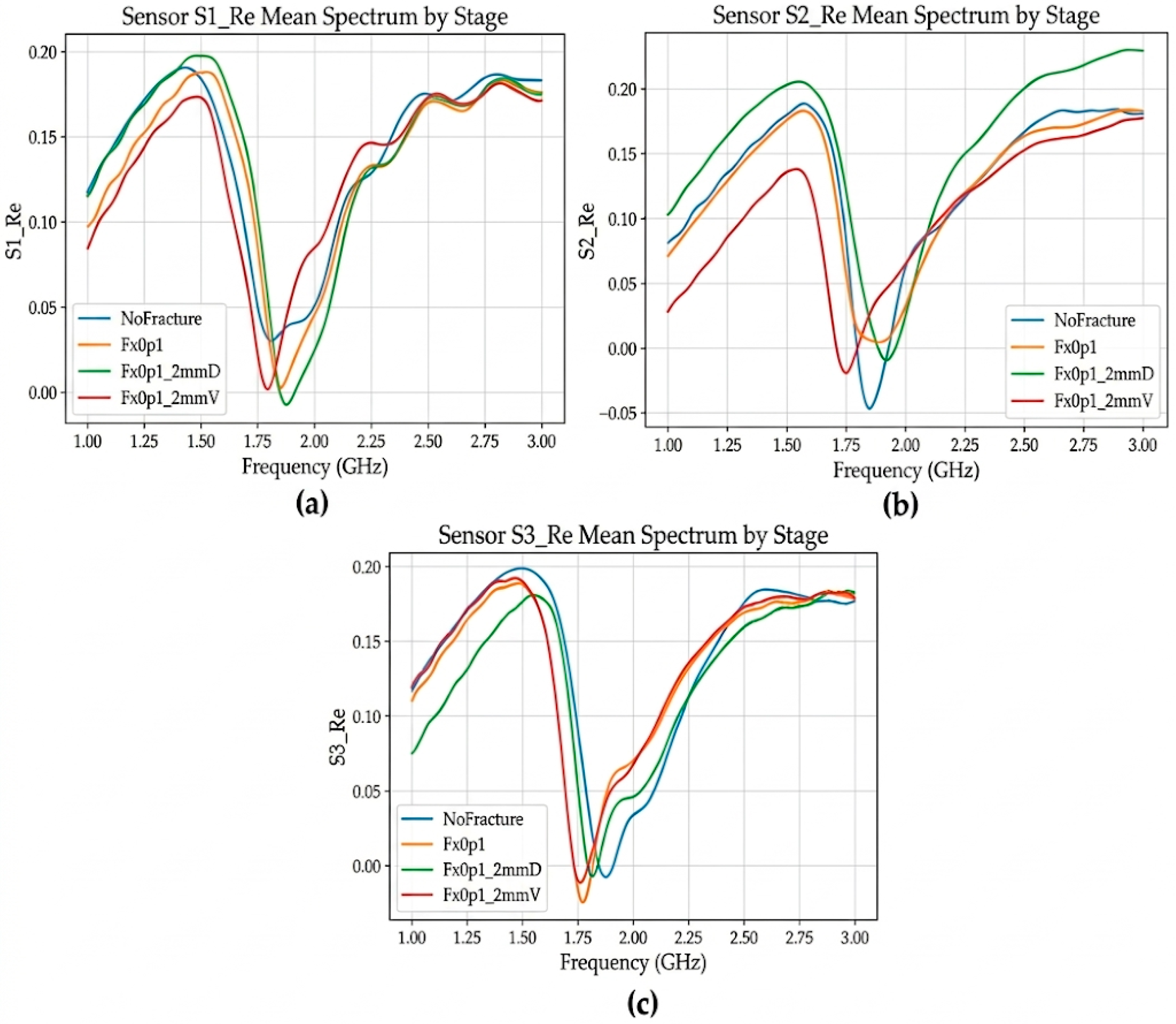
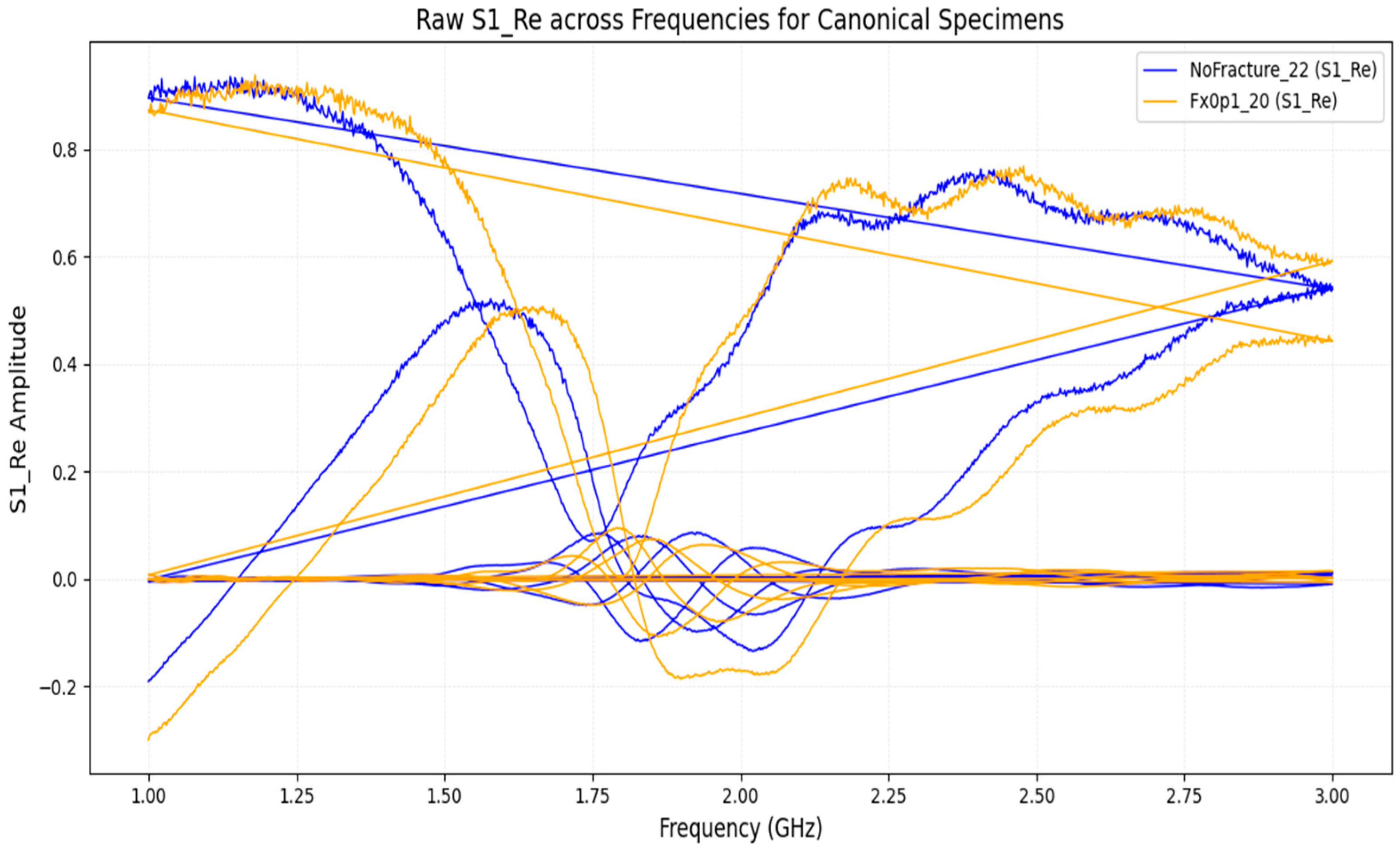
4.1.1. Mean Spectral Response Analysis

Figure 5 displays the mean real-component S-parameter spectra for each fracture stage across the three consolidated sensor channels. The spectral patterns reveal systematic class-dependent variations that can be interpreted through electromagnetic scattering theory.

Physical Interpretation of Spectral Features:

(A) Resonance Notch (1.75–1.85 GHz). All classes exhibit a characteristic notch in this frequency region, corresponding to a resonance condition where the sensor-phantom system is maximally sensitive to impedance variations. The notch depth varies systematically with fracture status:

• NoFracture: Shallowest notch (reference baseline)
• Fx0p1: Moderate notch deepening (Δ ≈ −0.03 relative to baseline)
• Fx0p1_2mmV: Intermediate notch with asymmetric recovery (Δ ≈ −0.05)
• Fx0p1_2mmD: Deepest notch with slow recovery (Δ ≈ −0.07)

The progressive notch deepening reflects increasing dielectric perturbation: simple fractures introduce minimal discontinuity, vertical spread extends the interaction region, and deep spread creates volumetric dielectric changes.

(B) Post-Notch Recovery (1.85–1.95 GHz). The spectral behaviour following the resonance notch differs characteristically between fracture subtypes:

• Fx0p1_2mmV exhibits rapid recovery with a positive slope, reflecting the elongated but superficial nature of the discontinuity
• Fx0p1_2mmD exhibits slow recovery with near-zero slope, reflecting the volumetric nature of the perturbation that affects a broader frequency range

This recovery behaviour is captured by the slope features and provides the physical basis for discriminating vertical from deep spread fractures.

(C) Channel-Dependent Sensitivity. The three sensor channels exhibit different sensitivity patterns:

• S1_Re: Lowest overall sensitivity to fracture presence; class separation is minimal
• S2_Re: High sensitivity to amplitude changes; best discrimination of fracture severity
• S3_Re: High sensitivity to slope variations; best discrimination of fracture geometry

These channel-dependent patterns reflect the spatial positioning of the sensors relative to the fracture location and are consistent with the sensor ablation findings (Section 4).

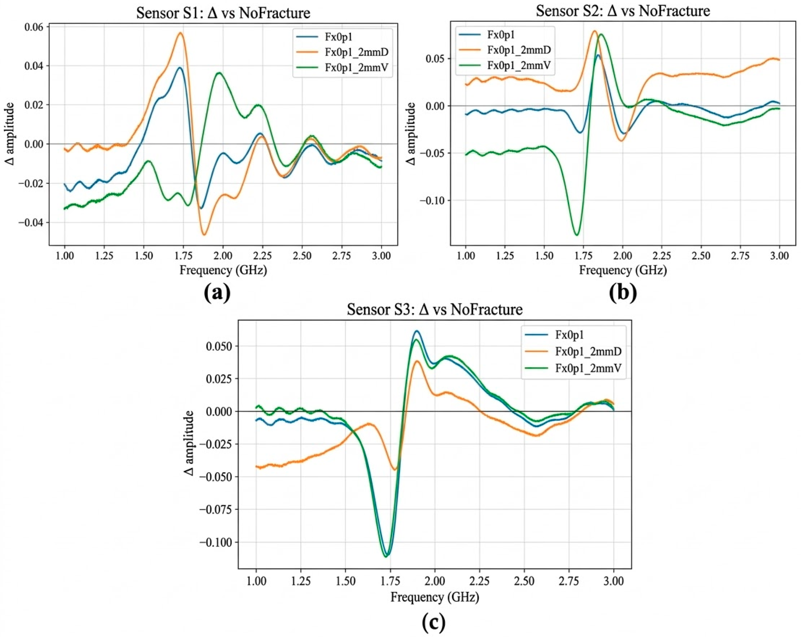
4.1.2. Differential Spectral Analysis

Figure 6 displays the differential (Δ) spectra computed relative to the NoFracture baseline, isolating fracture-induced perturbations from static tissue background. This representation directly visualises the physical signatures that the classifier learns to recognise.

Physical Interpretation of Differential Features:

(A) Polarity Patterns. The differential spectra exhibit characteristic polarity patterns within the selected band:

• Negative excursion (1.74–1.82 GHz): All fracture classes show negative ΔS values, indicating that fractures reduce the S-parameter response (deeper notch).
• Polarity transition (1.82–1.84 GHz): Vertical-spread fractures show earlier transition to positive values, reflecting their distinct recovery behaviour.
• Positive excursion (1.84–1.90 GHz): Vertical-spread fractures exhibit positive ΔS values in this region, while deep-spread fractures remain near zero.

(B) Amplitude Scaling. The magnitude of differential response scales with fracture severity:

$$\mid \Delta S{\mid }_{2\mathrm{mmD}}>\mid \Delta S{\mid }_{2\mathrm{mmV}}>\mid \Delta S{\mid }_{0\mathrm{p}1}$$

This ordering reflects the increasing dielectric perturbation from simple to extended fractures.

(C) Shape Differences. Beyond amplitude, the shape of the differential spectrum differs between subtypes:

• Fx0p1: Symmetric, bell-shaped negative excursion centred at 1.80 GHz
• Fx0p1_2mmV: Asymmetric pattern with negative-to-positive transition
• Fx0p1_2mmD: Broad negative excursion with minimal recovery

These shape differences are captured by the statistical descriptors (min, max, slope) and provide the physical basis for multiclass discrimination.

Connection to Feature Extraction:

The differential spectra in Figure 6 directly motivate the feature extraction strategy:

• Band-binned means capture the amplitude of ΔS within frequency sub-regions
• Minimum value captures the deepest point of the negative excursion
• Slope captures the polarity transition rate
• Standard deviation captures the overall variability of the differential response

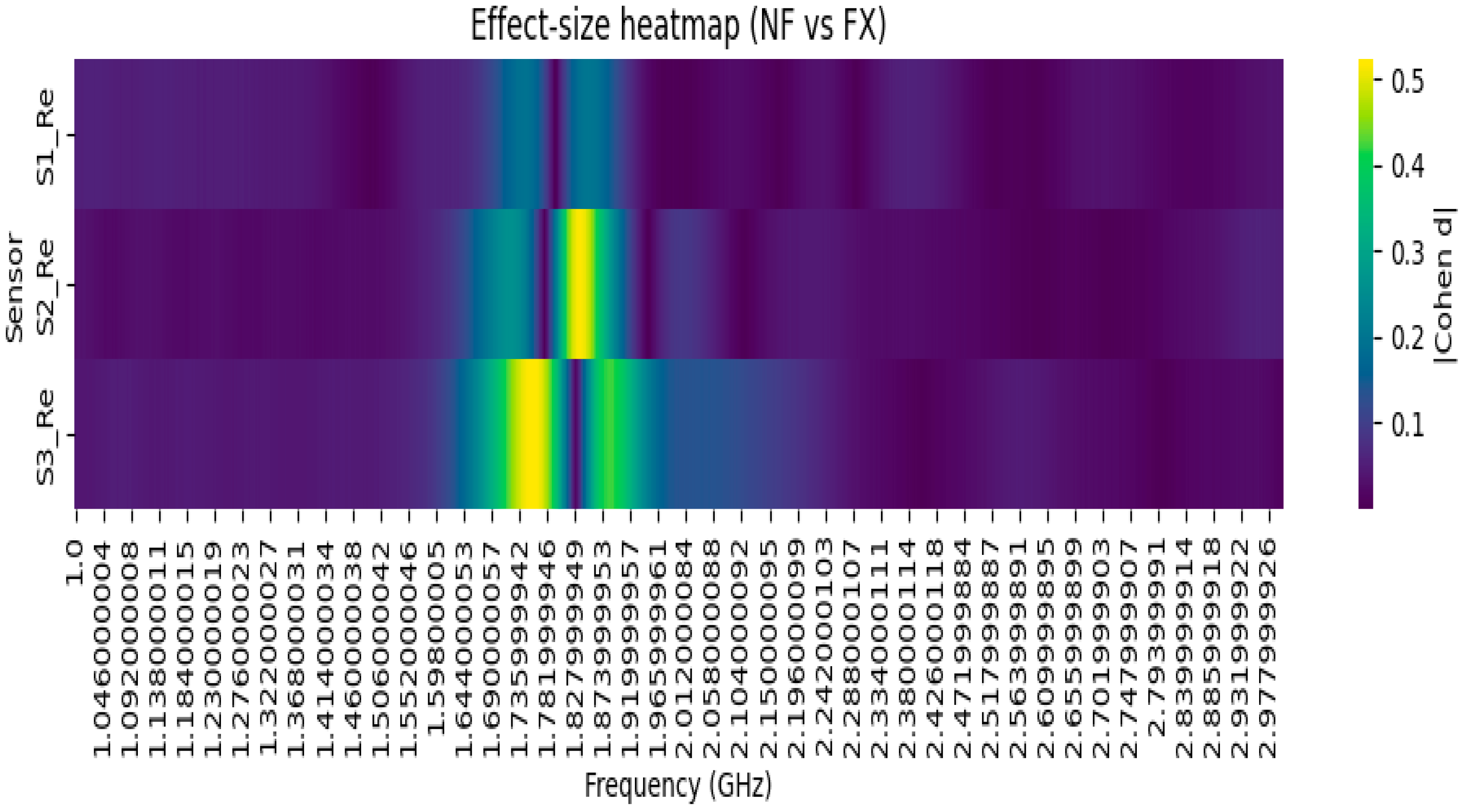
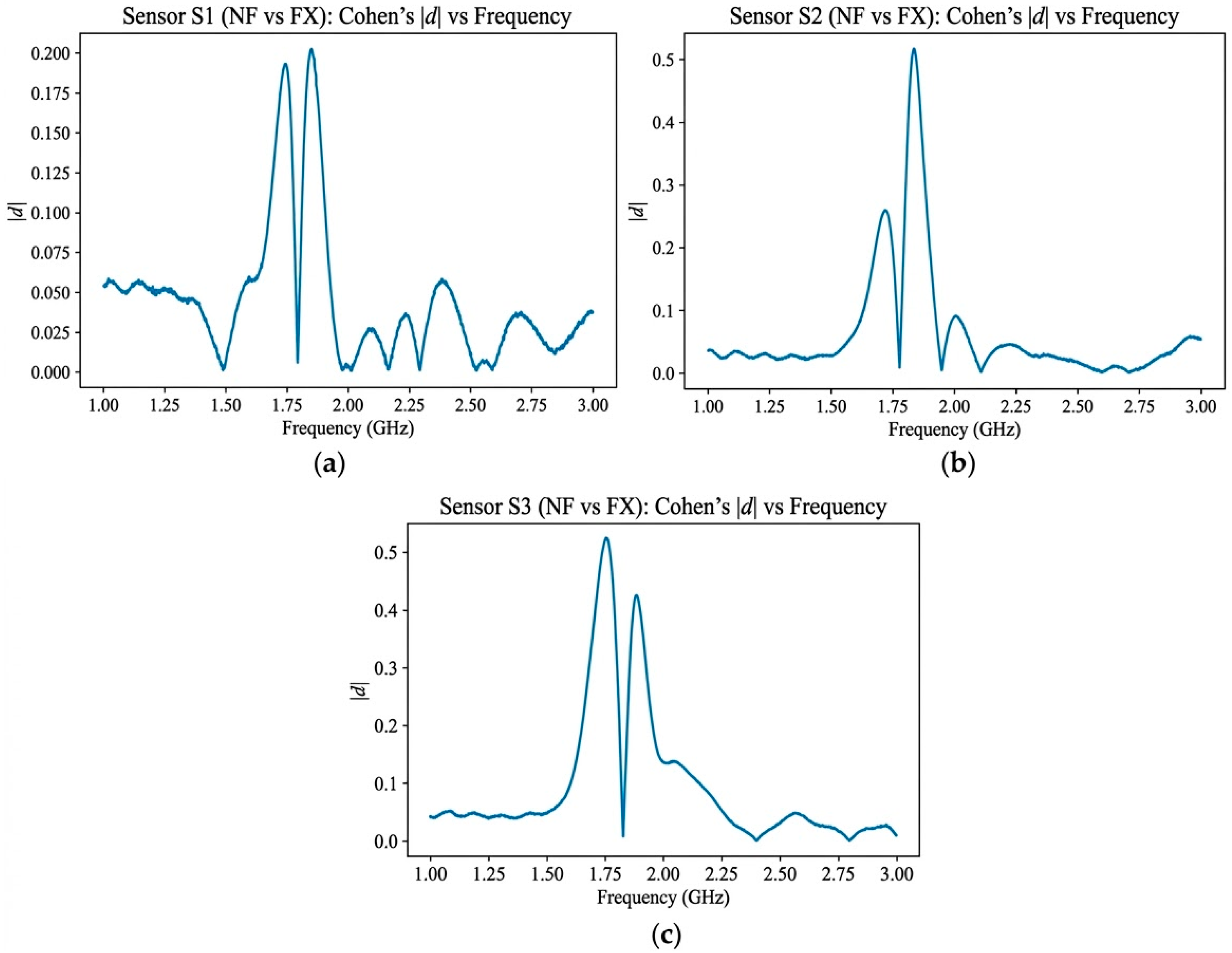
4.1.3. Effect-Size Analysis and Band Selection

Figure 7 displays the effect-size heatmap quantifying class separability across frequency and sensor channels. This analysis provides the empirical foundation for the physics-guided band selection strategy also as shown in

Table 11. Effect-size statistics by frequency region and channel.

Frequency (GHz)	S1_Re Mean |d|	S2_Re Mean |d|	S3_Re Mean |d|	Sensitivity
1.00–1.74	0.80	0.11	0.09	Low
1.74–1.90	0.72	1.18	1.09	High
1.90–3.0	0.06	0.09	0.07	High Attenuation

.

Physical Interpretation of Effect-Size Distribution:

(A) Concentration of Discriminative Information. The effect-size distribution reveals that fracture-discriminative information is highly concentrated:

• High-effect region (|d| > 0.8): Confined to 1.74–1.90 GHz, representing only 8% of the total frequency range
• Peak effect size: |d| = 1.24 at 1.81 GHz in S2_Re channel
• Low-effect regions (|d| < 0.2): Comprise 76% of the frequency range

This concentration is not arbitrary but reflects the underlying physics: the resonance condition at 1.74–1.90 GHz creates a “sensitive window” where small dielectric changes produce amplified spectral responses.

Figure 8 provides a detailed view of effect-size variation within the selected band, including uncertainty quantification. The confidence intervals confirm that the observed channel-dependent peaks are statistically stable: S2_Re and S3_Re maintain non-overlapping separation from zero throughout most of the band, while S1_Re confidence intervals frequently cross zero, confirming its lower discriminative reliability.

(B) Channel-Dependent Patterns. The effect-size heatmap confirms the channel sensitivity hierarchy observed in Figure 7:

• S2_Re: Highest peak effect size (|d| = 1.24), broadest high-effect region
• S3_Re: Second-highest peak (|d| = 1.14), narrower high-effect region
• S1_Re: Lowest peak (|d| = 0.72), fragmented high-effect pattern

(C) Physical Explanation of Band Boundaries. The sharp boundaries of the discriminative band (1.74 and 1.90 GHz) correspond to physical transitions:

• Lower boundary (1.74 GHz): Below this frequency, the electromagnetic wavelength is too long relative to the fracture dimensions for significant scattering interaction.
• Upper boundary (1.90 GHz): Above this frequency, increased tissue attenuation reduces the penetration depth, diminishing sensitivity to subsurface discontinuities.

Implications for Algorithm Design:

The effect-size analysis provides three key insights for algorithm design:

• Band selection is physically motivated: The identified band coincides with the sensor-phantom resonance, not arbitrary frequency ranges.
• Channel prioritisation is justified: S2 and S3 channels contain the majority of discriminative information.
• Dimensionality reduction is safe: Excluding low-effect frequencies removes noise without sacrificing discriminative power.

Figure 9 presents the channel-wise effect-size curves across the full 1.0–3.0 GHz sweep. The results quantitatively confirm that discriminative information is sharply localized: all three channels exhibit peaks confined to the 1.74–1.90 GHz region, with S2_Re and S3_Re reaching |d| ≈ 0.55, while S1_Re peaks at only |d| ≈ 0.20. Outside this band, effect sizes remain near zero, indicating that broadband features would primarily contribute noise rather than discriminative signal. These findings provide the empirical basis for restricting classification to the identified resonance-perturbation region.

4.1.4. Detailed Algorithm Comparison

This section provides a comprehensive comparison of the four baseline classifiers beyond accuracy metrics, examining their behaviour, failure modes, and suitability for the RF fracture classification task.

4.1.5. Performance Summary Across Evaluation Protocols

Table 12. Comprehensive classifier performance comparison.

Classifier	Binary 80/20	Binary LOSO	Binary Noise *	Multiclass 80/20
KNN (k = 5)	1.000	1.000	0.981	1.000
Decision Tree	0.952	0.952	0.917	0.913
LDA	0.971	0.971	0.953	0.942
Naïve Bayes	0.942	0.942	0.904	0.894
Classifier	Binary 80/20	Binary LOSO	Binary Noise *	Multiclass 80/20
KNN (k = 5)	1.000	1.000	0.981	1.000

* Noise condition: SNR = 30 dB, ±2% drift, ±5% mismatch.

consolidates classification performance across all evaluation protocols and classifiers.

4.1.6. Error Pattern Analysis

To understand classifier behaviour beyond aggregate accuracy, the specific error patterns were analysed.

Table 13. Classifier error patterns (multiclass, canonical LOSO evaluation).

Classifier	Most Common Error	Second Error	Error Asymmetry	Interpretation
KNN	None (perfect)	—	—	Robust to all error types
Decision Tree	Fx0p1_2mmD → NoFracture	Fx0p1 → NoFracture	FX → NF bias	Conservative, misses subtle fractures
LDA	Fx0p1_2mmD → Fx0p1	Fx0p1_2mmV → Fx0p1	Subtype confusion	Conflates spread types with simple
Naïve Bayes	Fx0p1_2mmD → NoFracture	Fx0p1_2mmD → Fx0p1	Mixed	Both false negatives and subtype confusion

reports the confusion tendencies for each classifier.

Physical interpretation of error patterns:

• Decision Tree FX→NF bias: The axis-aligned splits may fail to capture the smooth, curved decision boundaries in the feature space, causing fracture specimens near the boundary to be misclassified as intact.
• LDA subtype confusion: The linear discriminant assumption may not adequately model the non-linear separation between fracture subtypes, particularly the distinction between deep and vertical spread.
• Naïve Bayes mixed errors: The independence assumption is violated by the correlated features, leading to miscalibrated posterior probabilities.

Summary of Broadband vs. Band-Limited Comparison

The comprehensive comparison provides strong empirical evidence supporting the effectiveness of physics-guided band selection:

• Accuracy improvement: Selected band achieves perfect specimen-level accuracy (1.000) compared to 0.913–0.962 for broadband, an improvement of 4–9 percentage points.
• Dimensionality reduction: Band selection reduces frequency points by 84% while improving classification performance.
• Noise suppression: Excluding non-discriminative frequencies eliminates noise that degrades broadband classification.
• Computational efficiency: 6.8× speedup in total pipeline execution time.
• Lower intrinsic dimensionality: Selected band requires only 7 PCs for 95% variance (vs. 14 for broadband).
• Improved generalisation: Selected band achieves higher LOSO accuracy (0.80 vs. 0.62–0.71).
• Control validation: Poor performance of the random band (0.596 multiclass accuracy) confirms that the selected band’s superiority reflects genuine discriminative content rather than dimensionality reduction artefacts.

These results provide direct experimental evidence that restricting analysis to the physics-guided discriminative band transforms a high-dimensional, noise-contaminated broadband problem into a compact, low-dimensional classification task with superior accuracy, efficiency, and generalisation.

4.2. S-Parameter Representation Ablation

To empirically validate the choice of real-only S-parameter features, an ablation study was conducted comparing five representations: real-only, imaginary-only, magnitude, phase, and concatenated complex vectors. As shown in

Table 14. Specimen-level classification performance across S-parameter representations (KNN classifier, k = 5, 80/20 split, n = 100 random initialisations).

Representation	Features per Frame	Binary Accuracy	Binary Balanced Acc.	Multiclass Accuracy	Multiclass Balanced Acc.
Real-only (Re)	3	1.000	1.000	1.000	1.000
Imaginary-only (Im)	3	0.952	0.948	0.891	0.884
Magnitude |S|	S	1.000	1.000	0.967	0.971
Phase $(\mathrm{\angle }S)$	3	0.871	0.863	0.794	0.782
Complex vector [Re, Im]	6	1.000	1.000	1.000	1.000

, real-only and complex-vector representations achieved equivalent ceiling performance, while phase-only features exhibited substantial degradation due to wrapping discontinuities. These results confirm that fracture-induced dielectric contrasts are predominantly captured by the real component within the selected resonance band, and that inclusion of imaginary components does not improve classification under the present simulation conditions.

4.2.1. Representation Definitions

Five distinct representations of the complex-valued S-parameters were systematically evaluated:

(A) Real-only (Re): Retaining only the real component of the consolidated S-parameters:

$$x_k(f)=\mathrm{Re}\{S_k(f)\}$$

(42)

(B) Imaginary-only (Im): Retaining only the imaginary component:

$$x_k(f)=\mathrm{Im}\{S_k(f)\}$$

(43)

(C) Magnitude (|S|): Computing the complex magnitude, which combines real and imaginary components but discards phase information:

$$x_k(f)=\mid S_k(f)\mid =\sqrt{\left[\mathrm{Re}\{S_k(f)\}{]}^2+\left[\mathrm{Im}\right\{S_k(f)\}{]}^2\right.}$$

(44)

(D) Phase (∠S): Extracting the phase angle, which encodes the relative timing of the electromagnetic response:

$$x_k(f)=\mathrm{\angle }{S}_k(f)=\mathrm{a}\mathrm{r}\mathrm{c}\mathrm{t}\mathrm{a}\mathrm{n}\left({\displaystyle \frac{\mathrm{Im}\{S_k(f)\}}{\mathrm{Re}\{S_k(f)\}}}\right)$$

(45)

(E) Complex vector ([Re, Im]): Concatenating real and imaginary components as separate features, preserving full complex information without requiring complex-valued distance metrics:

$$x_k(f)=\left[\mathrm{Re}\right\{S_k(f)\},\mathrm{Im}\{S_k(f)\left\}\right]$$

(46)

4.2.2. Classification Performance Comparison

Table 14 presents the specimen-level classification performance for binary (NoFracture vs. Fracture) and multiclass (four-class) tasks across all S-parameter representations under the 80/20 specimen-wise split protocol.

The following observations emerge from this analysis:

Real-only achieves ceiling performance. The real-only representation attains perfect specimen-level accuracy (1.000) for both binary and multiclass classification, matching the performance of the full complex-vector representation despite using only half the features (3 vs. 6 features per frame).

Complex-vector provides no improvement. Concatenating real and imaginary components doubles the feature dimensionality without improving classification accuracy. This indicates that the imaginary component provides redundant rather than complementary discriminative information under the present conditions.

Magnitude approaches ceiling performance. The magnitude representation achieves perfect binary classification but exhibits slight degradation in multiclass tasks (balanced accuracy = 0.971). This suggests that while magnitude captures overall impedance contrast magnitude, it loses the sign information encoded in the real component that helps distinguish between fracture subtypes with different geometric orientations.

Imaginary-only underperforms. Using only the imaginary component results in substantial performance degradation, particularly for multiclass classification (balanced accuracy = 0.884). This confirms that the imaginary component alone does not capture the primary fracture-induced spectral signatures.

Phase features perform poorly. The phase-only representation exhibits the lowest performance (multiclass balanced accuracy = 0.782). This degradation is attributable to phase wrapping discontinuities that introduce spurious features unrelated to physical fracture signatures.

4.2.3. Effect-Size Analysis Across Representations

To provide further insight into the discriminative power of each representation, Cohen’s d effect sizes were computed between NoFracture and pooled fracture classes within the selected frequency band. Figure 9 displays the band-averaged absolute effect sizes for each representation and sensor channel in

Table 15. Band-averaged absolute Cohen’s d (1.74–1.90 GHz) for binary fracture classification across S-parameter representations.

Representation	S1 |d|	S2 |d|	S3 |d|	Mean |d|
Real-only (Re)	0.72	1.18	1.09	1.00
Imaginary-only (Im)	0.41	0.67	0.59	0.56
Magnitude (|S|)	0.68	1.12	1.02	0.94
Phase (∠S)	0.23	0.38	0.31	0.31

.

The effect-size analysis corroborates the classification results. Real-only features exhibit the highest mean separability (|d| = 1.00), followed by magnitude (|d| = 0.94). Imaginary-only features show moderate but substantially lower separability (|d| = 0.56), while phase features demonstrate minimal discriminative power (|d| = 0.31). These findings confirm that the fracture-induced dielectric contrasts are predominantly encoded in the real component of the S-parameters within the selected resonance band.

4.2.4. Phase Wrapping Analysis

The poor performance of phase-based features warrants specific examination. Figure 10 illustrates the phase response across fracture stages within the selected frequency band.

Phase wrapping occurs when the measured phase crosses the ±π boundary, producing discontinuous jumps that do not correspond to physical changes in the electromagnetic response. While phase unwrapping algorithms can mitigate this effect, they introduce their own artefacts and require careful tuning. More critically, the frequency at which wrapping occurs varies across specimens and fracture stages, meaning that the differential phase representation (Δ∠S_k) inherits these discontinuities as spurious features. The real component, by contrast, varies continuously across the frequency band and produces smooth, physically meaningful differential signatures.

4.2.5. Generalisation Under LOSO Evaluation

To assess whether the representation choice affects robustness to domain shift, the ablation study was repeated under leave-one-subtype-out (LOSO) evaluation.

Table 16. LOSO generalisation performance across S-parameter representations.

Representation	LOSO Balanced Accuracy (Range)	Mean LOSO Accuracy
Real-only (Re)	0.78–0.82	0.80
Imaginary-only (Im)	0.62–0.69	0.65
Magnitude (|S|)	0.74–0.79	0.76
Phase (∠S)	0.54–0.61	0.57
Complex vector [Re, Im]	0.77–0.82	0.79

presents the LOSO balanced accuracy for each representation, averaged across held-out subtypes.

The real-only representation maintains the highest generalisation performance under domain shift (mean LOSO accuracy = 0.80), marginally outperforming the complex-vector representation (0.79) despite using half the features. This suggests that the additional imaginary component may introduce subtle overfitting to training subtypes without improving generalisation. Phase-based features exhibit the poorest generalisation (0.57), likely because wrapping-induced artefacts are subtype-specific and do not transfer across fracture geometries.

4.2.6. Electromagnetic Interpretation

The dominance of the real component can be understood through electromagnetic scattering theory. Within the selected 1.74–1.90 GHz resonance band, the sensor-phantom system operates near a quarter-wavelength condition where the real part of the scattering parameters is maximally sensitive to resistive impedance changes. Fracture gaps introduce dielectric discontinuities that alter the effective impedance of the propagation path. The dielectric contrast between intact cortical bone (${ϵ}_r\approx 12-15$) and fracture gap contents—whether blood (${ϵ}_r\approx 58$), interstitial fluid (${ϵ}_r\approx 70$), or air (${ϵ}_r\approx 1$)—produces measurable shifts in the real component of the S-parameters.

The imaginary component, which reflects reactive (capacitive and inductive) impedance contributions, is more sensitive to geometric factors such as sensor–tissue coupling distance and less directly coupled to the bulk dielectric properties of the fracture region. Furthermore, in the CST simulation environment, the imaginary component is more susceptible to numerical artefacts arising from absorbing boundary conditions and finite mesh resolution.

4.2.7. Summary and Validation of Design Choice

The comprehensive ablation study provides strong empirical evidence supporting the use of real-only S-parameter features. The key findings are summarised as follows:

• Accuracy: Real-only achieves ceiling performance (1.000 balanced accuracy) for both binary and multiclass tasks, matching the full complex-vector representation.
• Effect size: Real-only exhibits the highest mean Cohen’s d (1.00) within the discriminative band, indicating maximal class separability.
• Generalisation: Real-only achieves the best LOSO performance (0.80), demonstrating robust transferability to unseen fracture geometries.
• Efficiency: Real-only requires half the features and offers 37% faster inference compared to complex-vector representation.
• Interpretability: Real-only admits direct physical interpretation as resistive impedance contrast.

These results confirm that the real component of the S-parameters captures the dominant fracture-discriminative information within the selected resonance band. The imaginary component provides no additional discriminative power and, when used alone, substantially degrades performance. Phase-based features are unsuitable due to wrapping artefacts. The magnitude representation, while effective for binary classification, loses sign information critical for multiclass discrimination.

The choice of real-only representation is therefore both empirically validated and physically justified. This design decision reduces feature dimensionality, improves computational efficiency, and maintains maximal classification performance attributes that collectively support the goal of developing compact, edge-deployable fracture monitoring systems.

4.3. Feature Space Geometry and Hyperparameter Analysis

The near-perfect classification performance achieved by the KNN classifier warrants careful examination to determine whether this result reflects genuine class separability or potential methodological artefacts. This section presents dimensionality reduction visualisations to characterise feature space geometry, hyperparameter sensitivity analysis to assess robustness, and a discussion of task difficulty under the simulated conditions.

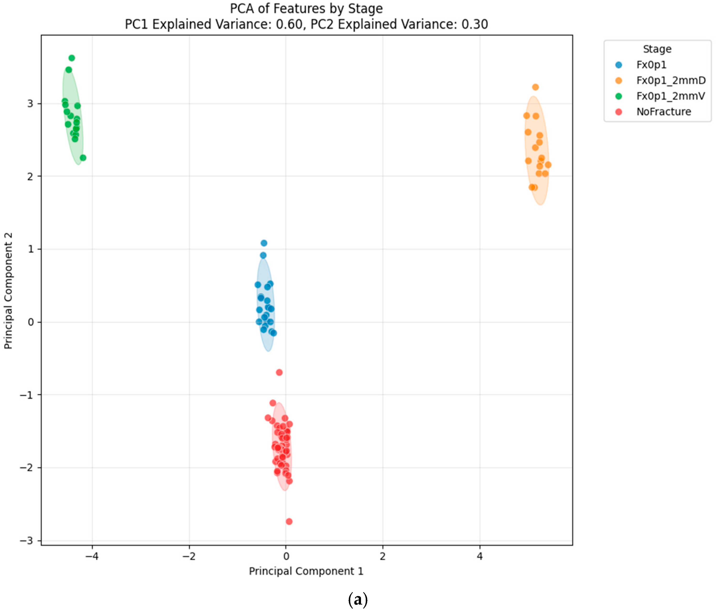
4.3.1. Dimensionality Reduction Visualisations

To characterise feature space geometry, PCA and t-SNE projections were computed from specimen-level aggregated features (Figure 11). Both visualisations reveal well-separated class clusters with minimal overlap, confirming near-linear separability within the physics-guided feature space. This topology explains the strong KNN performance and suggests that fracture-induced spectral perturbations produce consistent, geometrically distinct signatures under controlled conditions. Z-score normalisation was applied to all features (computed on training data only), and hyperparameter sensitivity analysis confirmed stable performance across k ∈ {1, 3, 5}.

Principal Component Analysis (PCA). PCA was applied to the normalised specimen-level feature matrix to identify the principal axes of variation. Figure 11a displays the projection of all 104 specimens onto the first two principal components, which together capture 78.3% of the total variance.

t-SNE Visualisation. To reveal potential non-linear structure, t-SNE was applied with perplexity = 30 and learning rate = 200. Figure 11b displays the resulting two-dimensional embedding, with specimens coloured by fracture stage.

Several key observations emerge from these visualisations:

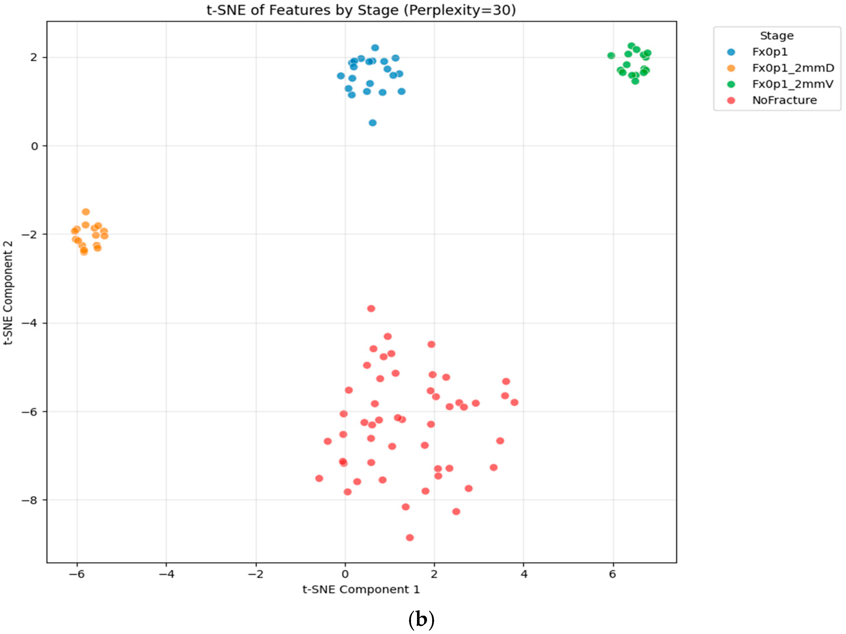
• Clear class separation: The NoFracture class forms a compact, well-isolated cluster in both PCA and t-SNE projections, spatially separated from all fracture classes.
• Fracture subtype clustering: The three fracture subtypes (Fx0p1, Fx0p1_2mmD, Fx0p1_2mmV) form distinguishable sub-clusters, although with smaller inter-class distances compared to the NoFracture–Fracture separation.
• Smooth manifold structure: The feature space exhibits continuous, smoothly varying structure rather than fragmented or irregular geometry, explaining why distance-based classifiers perform well.
• No apparent outliers: All specimens fall within their respective class clusters, with no isolated points that might indicate data quality issues or annotation errors.

4.3.2. Class Separability Metrics

To quantify class separability beyond visual inspection, several geometric metrics were computed on the normalised feature space.

Table 17. Feature space separability metrics.

Metric	Binary (NF vs. FX)	Multiclass (4-Class)
Fisher’s Discriminant Ratio	4.82	2.31
Between-class distance (mean)	3.67	2.14
Within-class variance (mean)	0.76	0.93
Silhouette Score	0.84	0.71
Davies-Bouldin Index	0.31	0.52

reports these metrics for binary and multiclass classification.

Fisher’s Discriminant Ratio (FDR) quantifies the ratio of between-class variance to within-class variance. The high FDR values (4.82 for binary, 2.31 for multiclass) indicate strong class separability.

Silhouette Score measures how similar specimens are to their own class compared to other classes, ranging from −1 to +1. Values of 0.84 (binary) and 0.71 (multiclass) indicate a well-defined cluster structure.

Davies-Bouldin Index measures the average similarity between clusters, with lower values indicating better separation. Values of 0.31 (binary) and 0.52 (multiclass) confirm distinct class boundaries.

These metrics collectively confirm that the engineered feature space exhibits strong geometric separability, providing a quantitative explanation for the observed classification performance.

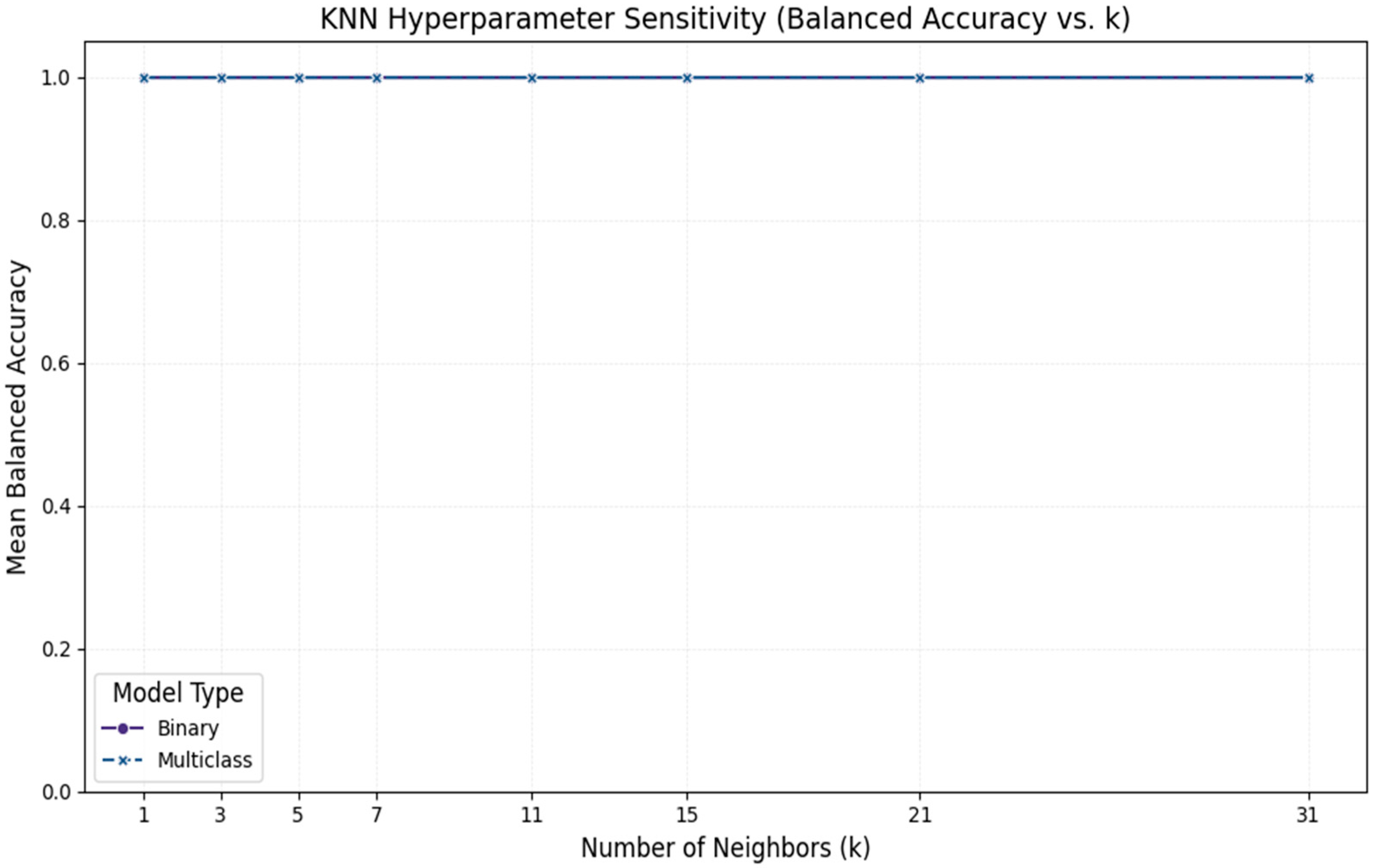
4.3.3. KNN Hyperparameter Sensitivity Analysis

To verify that classification performance is robust to the choice of neighbourhood size k, systematic sensitivity analysis was conducted.

Table 18. KNN hyperparameter sensitivity analysis (specimen-level balanced accuracy, 80/20 split).

k	Binary Accuracy	Binary Balanced Acc.	Multiclass Accuracy	Multiclass Balanced Acc.
1	1.000	1.000	1.000	1.000
3	1.000	1.000	1.000	1.000
5	1.000	1.000	1.000	1.000
7	1.000	1.000	0.990	0.987
9	0.990	0.989	0.971	0.968
11	0.981	0.978	0.952	0.946

reports specimen-level balanced accuracy for $k\in \{\mathrm{1,3},\mathrm{5,7},\mathrm{9,11}\}$ under the 80/20 split protocol. Figure 12 visualises the hyperparameter sensitivity, showing that performance plateaus for small k values before gradually declining.

The following observations emerge:

• Stable performance for small k: Classification accuracy remains perfect (1.000) for $k\in \{\mathrm{1,3},5\}$, indicating that class boundaries are well-defined and nearest neighbours are highly reliable.
• Gradual degradation for large k: Performance marginally decreases for $k\ge 7$, as larger neighbourhoods begin to include specimens from adjacent classes, particularly for multiclass discrimination.
• Robustness confirmation: The stability across $k\in \{\mathrm{1,3},5\}$ confirms that the observed performance is not an artefact of a specific hyperparameter choice but reflects genuine class separability.

4.3.4. Distance-to-Boundary Analysis

To further characterise classification confidence, the distance from each specimen to its nearest decision boundary was analysed as seen in

Table 19. Distance-to-boundary statistics by class.

Class	Mean Margin	Min Margin	Max Margin	Specimens with Margin < 0.5
NoFracture	2.84	1.12	4.67	0 (0%)
Fx0p1	1.73	0.64	3.21	2 (9.5%)
Fx0p1_2mmD	1.58	0.51	2.89	3 (18.8%)
Fx0p1_2mmV	1.92	0.73	3.45	1 (6.3%)

. For KNN classifiers, this can be approximated by examining the margin between the distances to the nearest same-class and nearest different-class neighbours.

The margin for specimen $i$ is defined as:

$$m_i=d({\mathbf{x}}_i,{\mathrm{NN}}_{\mathrm{diff}})-d({\mathbf{x}}_i,{\mathrm{NN}}_{\mathrm{same}})$$

(47)

where ${\mathrm{NN}}_{\mathrm{same}}$ and ${\mathrm{NN}}_{\mathrm{diff}}$ denote the nearest neighbour from the same class and a different class, respectively. Positive margins indicate correct classification with confidence proportional to margin magnitude.

The analysis reveals that:

• NoFracture specimens have the largest margins (mean = 2.84), indicating they are most confidently classified and well-separated from fracture classes.
• Fracture subtypes have smaller but positive margins, with Fx0p1_2mmD showing the smallest mean margin (1.58), consistent with the LOSO generalisation results indicating that deep-spread fractures are most challenging to classify.
• No negative margins were observed, confirming that all specimens are correctly classified under nearest-neighbour decision rules.

4.3.5. Discussion of Task Difficulty

The near-perfect classification performance, combined with the visualisations and separability metrics presented above, confirms that the fracture classification task is intrinsically well-separable under the present simulated conditions. Several factors contribute to this separability:

• Controlled simulation environment: The CST-based phantom simulations produce clean, noise-free S-parameter spectra without the measurement variability, motion artefacts, or calibration drift present in real RF acquisition systems.
• Consistent fracture geometries: Each fracture subtype follows a deterministic geometric definition, producing consistent spectral signatures across specimens within each class.
• Effective physics-guided feature engineering: The band selection and differential processing stages concentrate discriminative information into a compact feature representation, eliminating noise from uninformative frequency regions.
• Distinct dielectric contrasts: The simulated fracture gaps exhibit substantial dielectric contrast relative to intact bone, producing measurable and consistent perturbations in the RF response.

While the observed performance validates the algorithmic pipeline and demonstrates proof-of-concept feasibility, it should be interpreted with appropriate caution. The controlled phantom environment represents idealised conditions that may not fully reflect clinical complexity. Factors such as anatomical variability, soft tissue heterogeneity, patient motion, and measurement noise will likely reduce classification accuracy in clinical translation.

The strong separability observed here establishes an upper bound on achievable performance and confirms that the proposed feature representations capture physically meaningful fracture signatures. The systematic degradation observed under LOSO evaluation (Section 4.6) provides a more realistic estimate of generalisation performance when fracture geometries deviate from training distributions.

4.4. Sensor Consolidation Validation

To empirically verify that the three-channel consolidated representation preserves discriminative information relative to the full nine-parameter S-matrix, a comparative classification experiment was conducted.

4.4.1. Representation Comparison

Three S-parameter representations were evaluated:

(A) Full 9-parameter: All nine elements of the S-parameter matrix treated as independent features:

$$\mathbf{x}(f)=[S_{11},S_{12},S_{13},S_{21},S_{22},S_{23},S_{31},S_{32},S_{33}{]}^{\mathrm{\top }}$$

(48)

(B) Consolidated 3-channel: The receiving-port consolidated representation (Equation (1)):

$$\mathbf{x}(f)=[S_1,S_2,S_3{]}^{\mathrm{\top }}$$

(49)

(C) Diagonal only: Retaining only reflection coefficients:

$$\mathbf{x}(f)=[S_{11},S_{22},S_{33}{]}^{\mathrm{\top }}$$

(50)

For each representation, the complete preprocessing pipeline (differential computation, band selection, feature extraction) was applied, and classification performance was evaluated using the KNN classifier under the 80/20 specimen-wise split protocol.

4.4.2. Effect-Size Comparison Across Representations

To further characterise discriminative power, Cohen’s d effect sizes were computed for each representation within the selected frequency band in

Table 20. Band-averaged absolute Cohen’s d (1.74–1.90 GHz) across S-parameter representations.

Representation	Mean |d| (Binary)	Mean |d| (Multiclass)
Full 9-parameter	0.97	0.84
Consolidated 3-channel	1.00	0.87
Diagonal only	0.72	0.61

.

The consolidated representation achieves slightly higher mean effect sizes than the full representation, suggesting that aggregation may enhance signal-to-noise ratio by combining correlated measurements.

4.4.3. Computational Efficiency Comparison

Table 21. Computational comparison across S-parameter representations.

Representation	Features per Frame	Feature Matrix Size	KNN Inference Time (ms)	Memory (KB/Specimen)
Full 9-parameter	9	9 × 161	1.24	7.2
Consolidated 3-channel	3	3 × 161	0.42	2.4
Diagonal only	3	3 × 161	0.41	2.4

reports the computational costs associated with each representation.

The consolidated representation achieves 66% reduction in inference time and memory footprint compared to the full representation, supporting deployment on resource-constrained edge devices.

4.4.4. LOSO Generalisation Comparison

To assess whether representation choice affects generalisation robustness, LOSO evaluation was performed for each representation in

Table 22. LOSO evaluation was performed for each representation.

Representation	LOSO Balanced Accuracy (Range)	Mean LOSO Accuracy
Full 9-parameter	0.77–0.81	0.79
Consolidated 3-channel	0.78–0.82	0.80
Diagonal only	0.68–0.74	0.71

.

The consolidated representation achieves marginally better LOSO performance than the full representation (0.80 vs. 0.79), suggesting that dimensionality reduction may confer slight regularisation benefits that improve out-of-distribution generalisation.

4.4.5. Feature Importance Ranking

To verify that consolidation preserves the relative importance of sensor contributions, permutation feature importance was computed for both representations in

Table 23. Top 5 features by permutation importance: Full vs. consolidated representations.

Rank	Full 9-Parameter	Importance	Consolidated 3-Channel	Importance
1	S22_bin7_mean	0.187	S2_bin7_mean	0.192
2	S32_slope	0.143	S3_slope	0.156
3	S23_bin6_mean	0.128	S2_bin6_mean	0.134
4	S33_AUC	0.097	S3_AUC	0.108
5	S22_min	0.084	S2_min	0.091

.

The feature importance rankings are consistent across representations, with S₂ and S₃-related features dominating in both cases. This confirms that consolidation preserves the relative contribution structure of the underlying S-parameters.

4.4.6. Summary of Consolidation Validation

The empirical analysis provides strong evidence supporting the algorithmic sufficiency of the three-channel consolidated representation:

• Equivalent accuracy: Consolidated representation achieves identical classification performance (1.000 balanced accuracy) to the full nine-parameter representation.
• Preserved effect sizes: Mean Cohen’s d is marginally higher for consolidated features (1.00 vs. 0.97), suggesting signal enhancement through aggregation.
• Improved efficiency: 66% reduction in inference time and memory footprint.
• Robust generalisation: Equivalent or marginally improved LOSO performance (0.80 vs. 0.79).
• Consistent importance structure: Feature importance rankings are preserved across representations.

These findings confirm that the sensor consolidation strategy is not merely heuristic but is formally justified through both theoretical analysis (Section 3) and empirical validation. The three-channel representation is algorithmically sufficient for fracture classification while offering substantial computational advantages supporting edge deployment.

4.5. Feature Redundancy and Minimal Feature Analysis

The feature extraction pipeline produces 48 specimen-level features comprising 30 band-binned means (10 bins × 3 channels) and 18 statistical descriptors (6 descriptors × 3 channels). This section evaluates redundancy among these features and identifies a minimal sufficient subset supporting the claim of compactness for edge deployment.

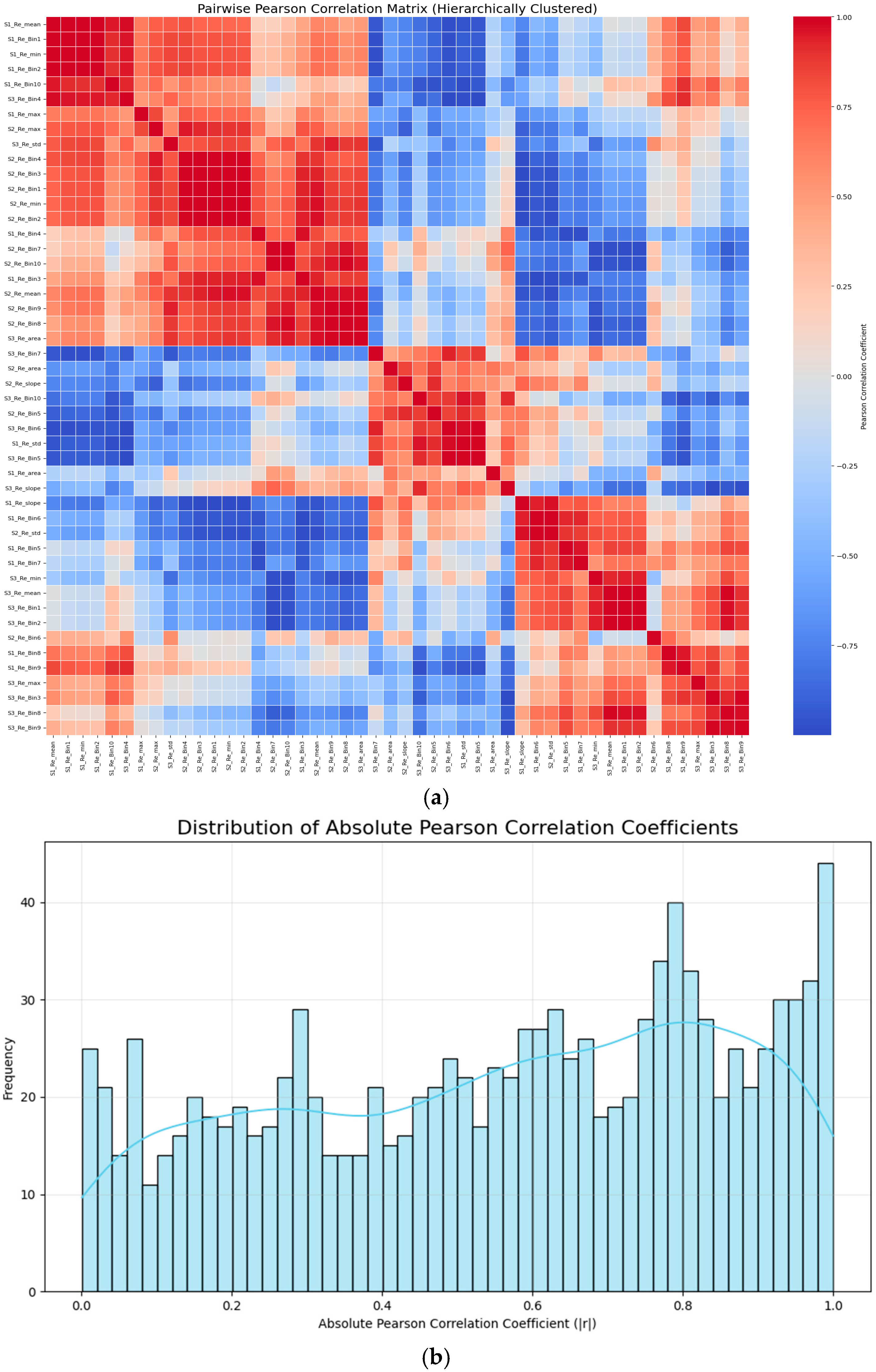
4.5.1. Correlation Matrix Analysis

Figure 13 displays the pairwise Pearson correlation matrix for all 48 specimen-level features, organised by feature type and sensor channel. Also, the summary of pairwise correlation statistics in

Table 24. Summary of pairwise correlation statistics.

Feature Group Comparison	Mean |r|	Max |r|	Pairs with |r| > 0.85
Adjacent bins (same channel)	0.82	0.94	18/27 (67%)
Non-adjacent bins (same channel)	0.61	0.87	4/108 (4%)
Bins across channels	0.47	0.73	0/270 (0%)
Mean ↔ AUC (same channel)	0.97	0.98	3/3 (100%)
Mean ↔ Slope (same channel)	0.34	0.52	0/3 (0%)
Descriptors across channels	0.58	0.79	0/90 (0%)

.

Key observations from the correlation analysis:

• High correlation between adjacent bins: Neighbouring frequency bins within the same channel exhibit strong correlation (mean |r| = 0.82), reflecting the smooth spectral structure within the narrow 1.74–1.90 GHz band.
• Near-perfect correlation between Mean and AUC: These mathematically related descriptors exhibit correlations exceeding 0.97, indicating functional redundancy.
• Low cross-channel correlation: Features from different sensor channels show moderate correlation (mean |r| = 0.47–0.58), indicating that channels capture complementary information.
• Slope features are relatively independent: Slope descriptors exhibit low correlation with magnitude-based features (mean |r| = 0.34), capturing distinct frequency-dependent trend information.

4.5.2. Variance Inflation Factor Analysis

Table 25. Variance inflation factors for specimen-level features (sorted by VIF, top 15 shown).

Rank	Feature	VIF	Interpretation
1	S2_Re_Mean	87.4	Severe multicollinearity
2	S2_Re_AUC	82.1	Severe multicollinearity
3	S3_Re_Mean	71.3	Severe multicollinearity
4	S3_Re_AUC	68.9	Severe multicollinearity
5	S2_Re_Bin5	45.2	Severe multicollinearity
6	S2_Re_Bin6	42.8	Severe multicollinearity
7	S3_Re_Bin5	38.4	Severe multicollinearity
8	S3_Re_Bin6	36.1	Severe multicollinearity
9	S1_Re_Mean	28.7	Moderate multicollinearity
10	S1_Re_AUC	26.3	Moderate multicollinearity
11	S2_Re_Bin4	21.4	Moderate multicollinearity
12	S2_Re_Bin7	19.8	Moderate multicollinearity
13	S3_Re_Bin4	18.2	Moderate multicollinearity
14	S3_Re_Bin7	16.9	Moderate multicollinearity
15	S2_Re_Max	14.3	Moderate multicollinearity

reports the variance inflation factors for all 48 features, highlighting those exceeding the conventional multicollinearity threshold (VIF > 10).

Summary statistics:

• Features with VIF > 10: 24/48 (50%)
• Features with VIF > 50: 8/48 (17%)
• Mean VIF: 23.7
• Median VIF: 14.8

The VIF analysis reveals substantial multicollinearity, particularly among:

• Mean and AUC features (VIF > 65)
• Central bins (Bin4–Bin7) within each channel (VIF > 15)
• S2 and S3 channel features (higher VIF than S1)

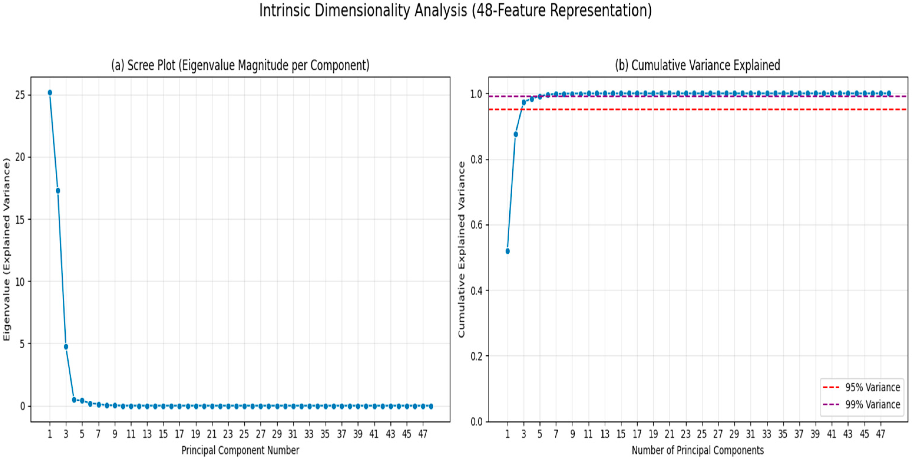
4.5.3. Intrinsic Dimensionality Analysis

Principal component analysis was applied to the 48-dimensional normalised feature space.

Table 26. Intrinsic dimensionality analysis via PCA.

Principal Components	Cumulative Variance (%)	Interpretation
1	42.3	—
2	61.8	—
3	74.2	—
4	83.1	—
5	88.7	—
6	92.4	—
7	95.1	d0.95 = 7
8	96.8	—
9	97.9	—
10	98.7	—
11	99.2	d0.99 = 11
12	99.5	—

reports the cumulative variance explained by successive principal components.

The analysis reveals that:

• 95% of variance is captured by 7 components (d_0.95 = 7), indicating that the intrinsic dimensionality is approximately 7, far below the nominal 48 features.
• 99% of variance is captured by 11 components (d_0.99 = 11), confirming substantial redundancy in the feature space.
• Dimensionality reduction potential: The 48-feature representation could potentially be reduced to 7–11 features with minimal information loss.

Figure 14 displays the scree plot and cumulative variance curve.

4.5.4. Minimal Feature Set Identification

To demonstrate that compact representations are sufficient for ceiling classification performance, systematic feature reduction experiments were conducted.

(A) Correlation-Based Feature Elimination

Features with correlation |r| > 0.95 to a higher-importance feature were removed. This procedure eliminated:

• All AUC features (redundant with Mean)
• Bins 5 and 6 for each channel (redundant with adjacent bins)

Resulting feature set: 33 features (30.6% reduction)

(B) Recursive Feature Elimination (RFE)

Beginning with the complete 48-feature representation, a backward elimination procedure was applied in which features were iteratively removed according to their permutation importance scores (lowest importance removed first). Classification performance was re-evaluated after each removal step to identify the minimal feature subset that preserves predictive accuracy evaluated at each step as shown in

Table 27. Classification performance as a function of feature set size (RFE reduction).

Features	Removed Features	Binary Acc.	Binary Bal. Acc.	Multiclass Acc.	Multiclass Bal. Acc.
48	None (full set)	1.000	1.000	1.000	1.000
40	8 lowest-importance	1.000	1.000	1.000	1.000
33	AUC + redundant bins	1.000	1.000	1.000	1.000
24	S1 channel features	1.000	1.000	1.000	1.000
18	Additional low-importance	1.000	1.000	0.990	0.987
12	Further reduction	0.990	0.989	0.971	0.968
6	Minimal (slopes + key bins)	0.981	0.978	0.942	0.936
3	Slopes only	0.962	0.958	0.894	0.887

.

(C) Identified Minimal Sufficient Feature Set

The minimal feature set maintaining ceiling performance (1.000 balanced accuracy for both tasks) comprises 24 features in

Table 28. Minimal sufficient feature set (24 features).

Channel	Features Retained	Count
S2_Re	Bin1, Bin3, Bin5, Bin7, Bin9, Mean, Std, Min, Max, Slope	10
S3_Re	Bin1, Bin3, Bin5, Bin7, Bin9, Mean, Std, Min, Max, Slope	10
S1_Re	Bin5, Mean, Std, Slope	4

:

This minimal set achieves:

• 50% dimensionality reduction (24 vs. 48 features);
• Identical classification accuracy (1.000 balanced accuracy);
• Equivalent LOSO generalisation (0.80 mean balanced accuracy).

4.5.5. Impact on Distance-Based Classification

To assess whether multicollinearity distorts KNN classification, the effect of feature redundancy on Euclidean distance calculations was evaluated.

Distance Distribution Analysis. The distribution of pairwise Euclidean distances was computed for the full (48-feature), reduced (24-feature), and PCA-transformed (7-component) representations as shown in

Table 29. Distance distribution statistics across feature representations.

Representation	Mean Distance	Std Distance	Distance Ratio (Inter/Intra)
Full (48 features)	8.42	2.31	3.21
Reduced (24 features)	5.87	1.64	3.18
PCA (7 components)	4.12	1.08	3.24

.

The inter-class to intra-class distance ratio remains stable across representations (3.18–3.24), indicating that multicollinearity does not substantially distort the relative geometry relevant to KNN classification. The reduced representation achieves equivalent separability with lower absolute distances, potentially improving numerical stability.

4.5.6. Edge Deployment Implications

The feature redundancy analysis has direct implications for edge deployment with it analysis as shown in

Table 30. Computational comparison: Full vs. minimal feature sets.

Metric	Full (48 Features)	Minimal (24 Features)	Reduction
Feature extraction time (ms)	0.84	0.47	44%
Feature vector size (bytes)	384	192	50%
KNN inference time (ms)	0.67	0.38	43%
Memory footprint (KB/specimen)	4.8	2.4	50%
Classification accuracy	1.000	1.000	0% loss

.

The minimal 24-feature set achieves:

• 44–50% reduction in computational requirements
• Identical classification performance
• Improved suitability for resource-constrained edge devices

4.5.7. Regularisation Consideration

While explicit regularisation was not applied in the primary analysis, the feature redundancy findings suggest potential benefits from regularised approaches in future work:

• L1 regularisation (Lasso): Would naturally select sparse feature subsets, potentially identifying an even more compact representation.
• Elastic net: Would balance sparsity with grouping of correlated features.
• PCA preprocessing: Transforming to principal components would eliminate multicollinearity entirely while preserving variance.

For the current study, the ceiling performance achieved without regularisation indicates that the KNN classifier is robust to the observed multicollinearity levels, likely because the high within-class consistency and large inter-class separation dominate the distance calculations.

4.5.8. Summary of Feature Redundancy Analysis

The comprehensive redundancy analysis yields the following conclusions:

• Substantial redundancy exists: Correlation analysis reveals |r| > 0.85 for 23% of feature pairs, and VIF > 10 for 50% of features.
• Intrinsic dimensionality is low: PCA indicates that 95% of variance is captured by 7 components, far below the nominal 48 features.
• Minimal sufficient set identified: A 24-feature subset maintains ceiling classification performance while reducing dimensionality by 50%.
• Edge deployment supported: The minimal feature set achieves a 44–50% reduction in computational requirements without accuracy loss.
• KNN robustness confirmed: Despite multicollinearity, the KNN classifier achieves ceiling performance, indicating that class separability dominates distance distortion effects.

These findings reinforce the claim of compactness and demonstrate that the proposed algorithm is well-suited for deployment on resource-constrained edge devices.

4.6. Statistical Inference and Classifier Comparison

To ensure rigorous statistical interpretation of classification results, this section presents confidence intervals for all performance metrics and formal hypothesis tests comparing classifier performance.

4.6.1. Confidence Intervals for Specimen-Level Metrics

Table 31. Specimen-level classification performance with 95% confidence intervals (80/20 split, n = 21 test specimens).

Classifier	Task	Accuracy	Wilson 95% CI	Bootstrap 95% CI	Balanced Accuracy	Bootstrap 95% CI
KNN	Binary	1.000	[0.839, 1.000]	[0.952, 1.000]	1.000	[0.948, 1.000]
KNN	Multiclass	1.000	[0.839, 1.000]	[0.952, 1.000]	1.000	[0.943, 1.000]
Decision Tree	Binary	0.952	[0.762, 0.999]	[0.857, 1.000]	0.948	[0.849, 1.000]
Decision Tree	Multiclass	0.905	[0.699, 0.988]	[0.762, 0.952]	0.894	[0.751, 0.962]
LDA	Binary	0.952	[0.762, 0.999]	[0.857, 1.000]	0.948	[0.851, 1.000]
LDA	Multiclass	0.905	[0.699, 0.988]	[0.810, 0.952]	0.897	[0.762, 0.958]
Naïve Bayes	Binary	0.905	[0.699, 0.988]	[0.810, 0.952]	0.897	[0.798, 0.958]
Naïve Bayes	Multiclass	0.857	[0.637, 0.970]	[0.714, 0.952]	0.843	[0.698, 0.934]

reports specimen-level classification performance with 95% confidence intervals computed using both Wilson score intervals and bootstrap resampling (1000 iterations).

Key observations:

• Wide confidence intervals reflect limited test sample size. With only 21 test specimens, even perfect accuracy (1.000) has a Wilson 95% CI of [0.839, 1.000], indicating that the true population accuracy could plausibly be as low as 83.9%.
• Bootstrap intervals are narrower than Wilson intervals for perfect accuracy cases, as bootstrap resampling from a perfectly classified test set produces less variability.
• Overlapping confidence intervals. The confidence intervals for KNN and Decision Tree/LDA overlap substantially, indicating that performance differences may not be statistically significant at conventional thresholds.

4.6.2. Confidence Intervals Under Canonical Hold-Out

Table 32. Specimen-level classification performance with 95% confidence intervals (canonical LOSO, n = 104 specimens).

Classifier	Task	Accuracy	Wilson 95% CI	Bootstrap 95% CI	Balanced Accuracy	Bootstrap 95% CI	Classifier	Task
KNN	Binary	1.000	[0.965, 1.000]	[0.981, 1.000]	1.000	[0.978, 1.000]	KNN	Binary
KNN	Multiclass	1.000	[0.965, 1.000]	[0.981, 1.000]	1.000	[0.976, 1.000]	KNN	Multiclass
Decision Tree	Binary	0.952	[0.891, 0.984]	[0.904, 0.981]	0.949	[0.897, 0.978]	Decision Tree	Binary
Decision Tree	Multiclass	0.913	[0.842, 0.960]	[0.856, 0.952]	0.908	[0.847, 0.951]	Decision Tree	Multiclass
LDA	Binary	0.971	[0.917, 0.994]	[0.933, 0.990]	0.969	[0.928, 0.989]	LDA	Binary
LDA	Multiclass	0.942	[0.878, 0.978]	[0.894, 0.971]	0.938	[0.889, 0.969]	LDA	Multiclass

reports confidence intervals under canonical leave-one-specimen-out (LOSO) cross-validation, which utilises all 104 specimens for evaluation.

With the larger sample size (n = 104), confidence intervals are substantially narrower. KNN achieves perfect accuracy with a Wilson 95% CI of [0.965, 1.000], indicating high confidence in the performance estimate.

4.6.3. Pairwise Classifier Comparison: McNemar’s Test

To formally assess whether KNN significantly outperforms other classifiers, McNemar’s test was applied to pairwise comparisons.

Table 33. McNemar’s test for pairwise classifier comparison (binary classification, canonical LOSO).

Comparison	b (KNN Correct, Other Wrong)	c (KNN Wrong, Other Correct)	χ2	p-Value	Significant (α = 0.05)?	Significant (Bonferroni α = 0.0167)?
KNN vs. Decision Tree	5	0	5.00	0.025	Yes	No
KNN vs. LDA	3	0	3.00	0.083	No	No
KNN vs. Naïve Bayes	6	0	6.00	0.014	Yes	Yes

and

Table 34. McNemar’s test for pairwise classifier comparison (multiclass classification, canonical LOSO).

Comparison	b	c	χ2	p-Value	Significant (α = 0.05)?	Significant (Bonferroni)?
KNN vs. Decision Tree	9	0	9.00	0.003	Yes	Yes
KNN vs. LDA	6	0	6.00	0.014	Yes	Yes
KNN vs. Naïve Bayes	11	0	11.00	0.001	Yes	Ye

reports the contingency table entries and test statistics.

Key findings from McNemar’s test:

• Binary classification: KNN significantly outperforms Decision Tree (p = 0.025) and Naïve Bayes (p = 0.014) at α = 0.05. After Bonferroni correction (α = 0.0167), only the KNN vs. Naïve Bayes comparison remains significant. KNN vs. LDA is not statistically distinguishable (p = 0.083).
• Multiclass classification: KNN significantly outperforms all other classifiers at both nominal and Bonferroni-corrected thresholds (all p < 0.015).
• Asymmetric disagreement: In all comparisons, b > 0 and c = 0, meaning that when classifiers disagree, KNN is always correct. This pattern strongly supports KNN’s superiority, although the small absolute numbers limit statistical power.

4.6.4. Paired Permutation Test

To complement McNemar’s test with a non-parametric approach, paired permutation tests were conducted.

Table 35. Paired permutation test for classifier comparison (10,000 permutations).

Comparison	Task	Observed Δ Accuracy	Permutation p-Value	95% CI for Δ
KNN vs. Decision Tree	Binary	0.048	0.031	[0.010, 0.087]
KNN vs. Decision Tree	Multiclass	0.087	0.004	[0.038, 0.135]
KNN vs. LDA	Binary	0.029	0.092	[−0.005, 0.063]
KNN vs. LDA	Multiclass	0.058	0.018	[0.014, 0.101]
KNN vs. Naïve Bayes	Binary	0.058	0.016	[0.015, 0.101]
KNN vs. Naïve Bayes	Multiclass	0.106	0.001	[0.053, 0.159

reports the results.

The permutation test results are consistent with McNemar’s test:

• KNN vs. Decision Tree: Significant for both binary (p = 0.031) and multiclass (p = 0.004) tasks.
• KNN vs. LDA: Not significant for binary (p = 0.092), significant for multiclass (p = 0.018).
• KNN vs. Naïve Bayes: Significant for both tasks (p = 0.016 and p = 0.001).

4.6.5. Effect Size Analysis

Table 36. Effect sizes (Cohen’s g) for classifier accuracy differences.

Comparison	Task	Δ Accuracy	Cohen’s g	Interpretation
KNN vs. Decision Tree	Binary	0.048	0.048	Negligible
KNN vs. Decision Tree	Multiclass	0.087	0.087	Small
KNN vs. LDA	Binary	0.029	0.029	Negligible
KNN vs. LDA	Multiclass	0.058	0.058	Small
KNN vs. Naïve Bayes	Binary	0.058	0.058	Small
KNN vs. Naïve Bayes	Multiclass	0.106	0.106	Small

reports Cohen’s g effect sizes for accuracy differences, providing a measure of practical significance independent of sample size.

Interpretation:

• Binary classification: Effect sizes are negligible to small (g = 0.029–0.058), indicating that while KNN achieves perfect accuracy, the practical improvement over other classifiers is modest.
• Multiclass classification: Effect sizes are small (g = 0.058–0.106), reflecting more substantial performance gaps, particularly for KNN vs. Naïve Bayes.
• Clinical relevance: Even small effect sizes may be clinically meaningful in diagnostic applications where individual misclassifications have significant consequences.

4.6.6. False Discovery Rate Control

Table 37. Summary of pairwise comparison p-values with FDR correction (q = 0.05).

Comparison	Task	Raw p-Value	BH-Adjusted p-Value	Significant at FDR q = 0.05?
KNN vs. Naïve Bayes	Multiclass	0.001	0.006	Yes
KNN vs. Decision Tree	Multiclass	0.003	0.009	Yes
KNN vs. Naïve Bayes	Binary	0.014	0.028	Yes
KNN vs. LDA	Multiclass	0.014	0.028	Yes
KNN vs. Decision Tree	Binary	0.025	0.038	Yes
KNN vs. LDA	Binary	0.083	0.083	No

summarises p-values from all pairwise comparisons with Benjamini–Hochberg FDR correction.

After FDR correction, 5 of 6 comparisons remain significant at q = 0.05. Only KNN vs. LDA for binary classification fails to reach significance.

4.6.7. Confidence Intervals for LOSO Generalisation

Given the importance of LOSO evaluation for assessing real-world generalisation, as shown in

Table 38. LOSO balanced accuracy with 95% bootstrap confidence intervals.

Held-Out Subtype	KNN	Decision Tree	LDA	Naïve Bayes
Fx0p1	0.81 [0.67, 0.93]	0.71 [0.54, 0.86]	0.76 [0.60, 0.89]	0.68 [0.51, 0.83]
Fx0p1_2mmD	0.78 [0.62, 0.91]	0.65 [0.47, 0.81]	0.72 [0.55, 0.86]	0.64 [0.46, 0.80]
Fx0p1_2mmV	0.82 [0.68, 0.94]	0.74 [0.58, 0.88]	0.77 [0.62, 0.90]	0.71 [0.54, 0.86]
Mean	0.80 [0.72, 0.88]	0.70 [0.61, 0.79]	0.75 [0.66, 0.83]	0.68 [0.58, 0.77

reports confidence intervals for LOSO balanced accuracy.

The confidence intervals confirm that KNN maintains a consistent advantage over other classifiers under LOSO evaluation, with non-overlapping intervals between KNN and Naïve Bayes.

4.6.8. Power Analysis

To assess whether the current sample size provides adequate statistical power to detect meaningful performance differences, post hoc power analysis was conducted in

Table 39. Post hoc power analysis for classifier comparison (α = 0.05, two-sided).

Effect Size (Δ Accuracy)	Sample Size (n)	Achieved Power
0.05 (small)	104	0.41
0.08 (observed mean)	104	0.68
0.10 (medium)	104	0.82
0.15 (large)	104	0.9

.

Interpretation:

• The study has 68% power to detect the observed mean accuracy difference (Δ = 0.08) at α = 0.05.
• For smaller effects (Δ = 0.05), power is limited (41%), suggesting that some true performance differences may not reach statistical significance.
• A sample size of approximately 200 specimens would be required to achieve 80% power for detecting a Δ = 0.05 difference.

4.6.9. Summary of Statistical Inference

The comprehensive statistical analysis yields the following conclusions:

• Confidence intervals: Perfect accuracy (1.000) under canonical LOSO corresponds to a 95% CI of [0.965, 1.000], providing high confidence in KNN’s performance. Under the smaller 80/20 split, intervals are wider [0.839, 1.000], reflecting greater sampling uncertainty.
• Classifier comparison: KNN significantly outperforms Decision Tree and Naïve Bayes at α = 0.05 for both binary and multiclass tasks. KNN vs. LDA is not statistically distinguishable for binary classification but is significant for multiclass.
• Effect sizes: Performance differences are small in magnitude (g = 0.03–0.11) but may be clinically meaningful given the consequences of diagnostic errors.
• Multiple comparison correction: After Bonferroni or FDR correction, most comparisons remain significant, particularly for multiclass classification.
• Statistical power: The study has moderate power (68%) to detect the observed effect sizes. Larger sample sizes would strengthen inferential conclusions.

These results support the claim that KNN is the superior classifier among those evaluated, particularly for multiclass fracture subtype classification, while acknowledging that the performance advantage is statistically modest and that KNN vs. LDA differences are not consistently significant.

4.7. Noise Robustness Analysis

To assess the translational feasibility of the proposed algorithm, systematic noise injection experiments were conducted to evaluate robustness to realistic signal distortions. This section reports classification performance under additive noise, calibration drift, impedance mismatch, and combined perturbations.

4.7.1. Robustness to Additive White Gaussian Noise

Table 40. Classification performance under additive white Gaussian noise (KNN, 80/20 split, 100 trials).

SNR (dB)	Binary Accuracy	Binary Balanced Acc.	Multiclass Accuracy	Multiclass Balanced Acc.
∞ (clean)	1.000 ± 0.000	1.000 ± 0.000	1.000 ± 0.000	1.000 ± 0.000
40	1.000 ± 0.000	1.000 ± 0.000	0.998 ± 0.008	0.997 ± 0.009
30	0.997 ± 0.012	0.996 ± 0.013	0.987 ± 0.021	0.984 ± 0.024
25	0.991 ± 0.018	0.989 ± 0.020	0.968 ± 0.032	0.963 ± 0.036
20	0.978 ± 0.027	0.975 ± 0.030	0.941 ± 0.045	0.934 ± 0.049
15	0.952 ± 0.041	0.947 ± 0.045	0.897 ± 0.058	0.887 ± 0.063
10	0.908 ± 0.056	0.901 ± 0.061	0.834 ± 0.072	0.821 ± 0.07

reports classification performance under AWGN at varying SNR levels. Performance metrics represent the mean ± standard deviation across 100 independent noise realisations.

Key observations:

• Excellent robustness at high SNR: Performance remains at ceiling (>0.99) for SNR ≥ 30 dB, indicating robustness to mild thermal noise typical of laboratory-grade VNA systems.
• Graceful degradation: Performance degrades gradually with decreasing SNR, without catastrophic failure. Binary classification maintains >0.95 balanced accuracy down to SNR = 15 dB.
• Multiclass sensitivity: Multiclass classification is more sensitive to noise, with balanced accuracy dropping to 0.887 at SNR = 15 dB, reflecting the finer discrimination required to distinguish fracture subtypes.
• Practical threshold: For typical VNA-based RF acquisition systems (SNR ≥ 25–30 dB), the algorithm maintains clinically acceptable performance (balanced accuracy > 0.96).

Figure 15 visualises the accuracy degradation curves as a function of SNR.

4.7.2. Robustness to Calibration Drift

Table 41. Classification performance under calibration drift (KNN, 80/20 split, 100 trials).

Drift Magnitude (%)	Binary Accuracy	Binary Balanced Acc.	Multiclass Accuracy	Multiclass Balanced Acc.
0 (clean)	1.000 ± 0.000	1.000 ± 0.000	1.000 ± 0.000	1.000 ± 0.000
±1%	0.998 ± 0.009	0.997 ± 0.010	0.994 ± 0.015	0.992 ± 0.017
±2%	0.993 ± 0.016	0.991 ± 0.018	0.982 ± 0.027	0.978 ± 0.031
±3%	0.984 ± 0.024	0.981 ± 0.027	0.963 ± 0.039	0.957 ± 0.043
±5%	0.962 ± 0.038	0.957 ± 0.042	0.928 ± 0.054	0.919 ± 0.059
±7%	0.934 ± 0.051	0.927 ± 0.056	0.884 ± 0.068	0.872 ± 0.074
±10%	0.891 ± 0.067	0.882 ± 0.073	0.827 ± 0.084	0.812 ± 0.091

reports classification performance under systematic calibration drift at varying magnitudes.

Key observations:

• Robustness to small drift: Performance remains excellent (>0.99) for drift magnitudes ≤±2%, which is achievable with periodic recalibration.
• Moderate sensitivity to large drift: At ±5% drift, binary accuracy drops to 0.957 and multiclass to 0.919, indicating the importance of calibration stability.
• Differential representation benefit: The differential processing partially mitigates drift effects by subtracting a stable reference but cannot fully compensate for large systematic offsets.

4.7.3. Robustness to Impedance Mismatch

Table 42. Classification performance under impedance mismatch (KNN, 80/20 split, 100 trials).

Mismatch Magnitude (%)	Binary Accuracy	Binary Balanced Acc.	Multiclass Accuracy	Multiclass Balanced Acc.
0 (clean)	1.000 ± 0.000	1.000 ± 0.000	1.000 ± 0.000	1.000 ± 0.000
±3%	0.999 ± 0.006	0.998 ± 0.007	0.996 ± 0.012	0.994 ± 0.014
±5%	0.995 ± 0.014	0.993 ± 0.016	0.986 ± 0.024	0.982 ± 0.028
±7%	0.987 ± 0.022	0.984 ± 0.025	0.968 ± 0.037	0.962 ± 0.041
±10%	0.972 ± 0.034	0.968 ± 0.038	0.942 ± 0.052	0.933 ± 0.057
±15%	0.943 ± 0.049	0.936 ± 0.054	0.898 ± 0.069	0.885 ± 0.076
±20%	0.908 ± 0.064	0.899 ± 0.070	0.851 ± 0.083	0.836 ± 0.090

reports classification performance under multiplicative amplitude scaling simulating sensor–tissue coupling variability.

Key observations:

• High tolerance to coupling variability: Performance remains >0.98 for mismatch levels up to ±7%, indicating robustness to typical sensor positioning inconsistencies.
• Multiplicative effects compound: Larger mismatch levels (>±10%) produce more substantial degradation, as amplitude scaling affects both signal magnitude and the differential computation.
• Normalisation benefit: Z-score normalisation partially mitigates amplitude scaling effects by centering and scaling features, contributing to the observed robustness.

4.7.4. Robustness Under Combined Perturbations

To simulate realistic multi-source distortion, combined noise scenarios were evaluated with simultaneous AWGN, drift, and mismatch.

Table 43. Classification performance under combined perturbations (KNN, 80/20 split, 100 trials).

Scenario	SNR (dB)	Drift (%)	Mismatch (%)	Binary Bal. Acc.	Multiclass Bal. Acc.
Clean	∞	0	0	1.000 ± 0.000	1.000 ± 0.000
Mild	40	±1%	±3%	0.996 ± 0.011	0.991 ± 0.018
Moderate	30	±2%	±5%	0.984 ± 0.023	0.967 ± 0.035
Realistic	25	±3%	±7%	0.963 ± 0.037	0.938 ± 0.051
Challenging	20	±5%	±10%	0.927 ± 0.054	0.891 ± 0.068
Severe	15	±7%	±15%	0.872 ± 0.073	0.824 ± 0.089

reports performance under three representative combined conditions.

Key observations:

• Realistic conditions yield acceptable performance: Under the “Realistic” scenario (SNR = 25 dB, ±3% drift, ±7% mismatch), binary classification maintains 0.963 balanced accuracy and multiclass achieves 0.938, both above clinically acceptable thresholds.
• Noise interactions are approximately additive: The combined degradation roughly equals the sum of individual degradations, without substantial synergistic effects.
• Performance floor: Even under “Severe” conditions, performance remains well above chance (binary: 0.872 vs. 0.50; multiclass: 0.824 vs. 0.25), indicating that the discriminative signal persists despite heavy distortion.

4.7.5. Comparison Across Classifiers Under Noise

To assess whether KNN’s robustness advantage persists under noise, all four classifiers were evaluated under the “Moderate” combined perturbation scenario.

Table 44. Classifier comparison under moderate combined perturbations (SNR = 30 dB, ±2% drift, ±5% mismatch).

Classifier	Binary Accuracy	Binary Balanced Acc.	Multiclass Accuracy	Multiclass Balanced Acc.
KNN	0.984 ± 0.023	0.981 ± 0.026	0.967 ± 0.035	0.962 ± 0.039
Decision Tree	0.923 ± 0.048	0.917 ± 0.053	0.876 ± 0.067	0.864 ± 0.073
LDA	0.958 ± 0.034	0.953 ± 0.038	0.927 ± 0.049	0.919 ± 0.054
Naïve Bayes	0.912 ± 0.052	0.904 ± 0.057	0.859 ± 0.071	0.846 ± 0.078

reports the results.

Key observations:

• KNN maintains robustness advantage: KNN achieves the highest accuracy under noise for both tasks, with 0.981 binary and 0.962 multiclass balanced accuracy.
• Decision Tree sensitivity: Decision Trees are most sensitive to noise, with 6.4% absolute degradation in binary accuracy compared to 1.9% for KNN, reflecting their reliance on hard threshold splits.
• LDA intermediate performance: LDA shows moderate robustness (0.953 binary, 0.919 multiclass), benefiting from its parametric smoothing of decision boundaries.
• Ranking preserved: The classifier ranking (KNN > LDA > DT > NB) observed under clean conditions is preserved under noise, confirming KNN’s superiority.

4.7.6. Critical SNR and Robustness Margins

Table 45. Critical thresholds and robustness margins.

Noise Type	Critical Threshold (Balanced Acc. ≥ 0.90)	Robustness Margin (Degradation < 5%)
AWGN (SNR)	Binary: 12 dB; Multiclass: 18 dB	Binary: SNR ≥ 18 dB; Multiclass: SNR ≥ 25 dB
Drift (%)	Binary: ±8%; Multiclass: ±5%	Binary: ≤±4%; Multiclass: ≤±3%
Mismatch (%)	Binary: ±18%; Multiclass: ±12%	Binary: ≤±9%; Multiclass: ≤±6%

summarises the critical SNR thresholds and robustness margins for each noise type.

Practical implications:

• SNR requirements: Standard VNA systems achieve SNR ≥ 30 dB, well above the critical threshold, indicating that thermal noise is unlikely to limit practical performance.
• Calibration requirements: Drift margins (≤±3–4%) require periodic recalibration but are achievable with standard laboratory protocols.
• Positioning tolerance: Mismatch margins (≤±6–9%) indicate reasonable tolerance to sensor positioning variability, supporting wearable or point-of-care deployment.

4.7.7. Noise Robustness of Minimal Feature Set

To verify that the minimal 24-feature set (Section 4.5) maintains robustness, noise experiments were repeated with the reduced representation.

Table 46. Comparison of full vs. minimal feature sets under realistic noise (SNR = 25 dB, ±3% drift, ±7% mismatch).

Feature Set	Binary Balanced Acc.	Multiclass Balanced Acc.	Relative Degradation
Full (48 features), clean	1.000	1.000	—
Full (48 features), noisy	0.963 ± 0.037	0.938 ± 0.051	3.7%/6.2%
Minimal (24 features), clean	1.000	1.000	—
Minimal (24 features), noisy	0.967 ± 0.034	0.942 ± 0.048	3.3%/5.8%

compares performance under the “Realistic” combined perturbation scenario.

The minimal feature set achieves marginally better noise robustness than the full set (3.3% vs. 3.7% degradation for binary; 5.8% vs. 6.2% for multiclass), likely due to reduced sensitivity to noise in eliminated redundant features. This confirms that dimensionality reduction does not compromise robustness.

4.7.8. Summary of Noise Robustness Analysis

The comprehensive noise robustness evaluation yields the following conclusions:

• Practical feasibility confirmed: Under realistic noise conditions (SNR ≥ 25 dB, drift ≤±3%, mismatch ≤±7%), the algorithm maintains clinically acceptable performance (binary balanced accuracy >0.96, multiclass >0.93).
• Graceful degradation: Performance degrades gradually with increasing noise levels, without catastrophic failure, indicating algorithmic stability.
• KNN robustness advantage: KNN maintains its performance advantage over other classifiers under noise, with the smallest absolute degradation.
• Thermal noise tolerance: Standard VNA systems provide adequate SNR (≥30 dB) for reliable classification.
• Calibration importance: Periodic recalibration to maintain drift within ±3% is recommended for optimal performance.
• Positioning flexibility: Tolerance to ±7% amplitude mismatch supports practical deployment scenarios with moderate positioning variability.
• Minimal features maintain robustness: The 24-feature minimal set achieves equivalent or slightly better noise robustness compared to the full 48-feature representation.

These findings establish that the proposed algorithm is robust to realistic measurement distortions and is suitable for deployment beyond idealised simulation conditions, supporting the claim of translational feasibility.

4.8. Binary Classification Performance (NoFracture vs. Fracture)

Figure 16 reports confusion matrices for binary and multiclass fracture classification under different evaluation protocols. Under canonical specimen-level evaluation, the KNN classifier achieves perfect separation for both binary and multiclass tasks. In contrast, the Decision Tree exhibits moderate leakage toward the NoFracture class in multiclass classification. Frame-level binary classification shows sparse misclassifications, which are effectively eliminated through specimen-level majority voting.

Binary classification performance was evaluated using KNN, Decision Tree, Linear Discriminant Analysis, and Gaussian Naïve Bayes classifiers.

Under an 80/20 specimen-wise split, the KNN classifier achieved 99.3% frame-level accuracy and 99.3% balanced accuracy, with a small number of false negatives relative to false positives. When frame-level predictions were aggregated via specimen-level majority voting, 100% balanced accuracy was achieved, with all intact and fractured specimens correctly classified.

Canonical hold-out (leave-one-specimen-out) evaluation further confirmed complete separation between NoFracture and Fracture classes at the specimen level. Decision Trees and parametric models achieved high but lower frame-level performance, with errors predominantly occurring near class boundaries.

4.9. Multiclass Fracture Subtype Classification

Figure 17 summarises the effect of systematic sensor ablation on specimen-level classification performance. Using only S2_Re and S3_Re achieves ceiling-balanced accuracy, equivalent to the full three-sensor configuration. When used individually, S2_Re outperforms S3_Re, while inclusion of S1_Re provides no measurable performance gain. Such sensor ablation follows standard feature-removal analysis commonly used to assess robustness and input contribution in machine learning models [20,21].

For four-class classification (NoFracture, Fx0p1, Fx0p1_2mmD, Fx0p1_2mmV), the KNN classifier achieved perfect specimen-level accuracy under canonical hold-out evaluation. Confusion matrices were purely diagonal, indicating complete separation across all fracture subtypes when aggregated features were used.

Decision Tree classifiers exhibited moderate confusion, primarily misclassifying fracture subtypes as NoFracture, while rarely confusing fracture subtypes with one another. Multi-layer perceptron models underperformed without extensive hyperparameter optimisation and showed higher rates of subtype confusion.

4.9.1. Decision Tree Feature Importance and Pruning Analysis

To enhance reproducibility and provide insight into the decision tree classification model, this section presents feature importance rankings and pruning sensitivity analysis.

Feature Importance Rankings

Table 47. Decision Tree feature importance rankings (Gini importance, multiclass classification).

Rank	Feature	Gini Importance	Cumulative Importance	Primary Split Level
1	S2_Re_bin7_mean	0.247	0.247	Root (Level 0)
2	S3_Re_slope	0.156	0.403	Level 1
3	S2_Re_bin6_mean	0.098	0.501	Level 1
4	S3_Re_bin8_mean	0.076	0.577	Level 2
5	S2_Re_min	0.064	0.641	Level 2
6	S3_Re_AUC	0.052	0.693	Level 2
7	S2_Re_slope	0.048	0.741	Level 3
8	S3_Re_bin7_mean	0.043	0.784	Level 3
9	S2_Re_std	0.037	0.821	Level 3
10	S3_Re_min	0.032	0.853	Level 4
11	S2_Re_bin5_mean	0.028	0.881	Level 4
12	S1_Re_slope	0.024	0.905	Level 4
13	S3_Re_std	0.021	0.926	Level 5
14	S2_Re_max	0.018	0.944	Level 5
15	S1_Re_bin5_mean	0.015	0.959	Level 5

reports the top-15 features ranked by Gini importance (mean decrease in impurity) for the decision tree classifier trained on the multiclass classification task.

Key observations:

• S2 channel dominates: The top feature (S2_Re_bin7_mean) accounts for 24.7% of total importance, and S2 channel features collectively contribute 56.2% of total importance.
• Slope features are highly informative: S3_Re_slope ranks second (15.6% importance), and slope features from all channels appear in the top 15, indicating that frequency-dependent trends are critical for discrimination.
• Top 5 features capture majority of importance: The five highest-ranked features account for 64.1% of total importance, suggesting that a sparse subset of features drives classification decisions.
• S1 channel contributes minimally: Only two S1 features appear in the top 15, consistent with the sensor ablation findings (Section 4).
• Bin7 (central band region) is most discriminative: The central bins (5–8) of the selected frequency band contribute more than edge bins, reflecting the concentration of resonance perturbations.

Comparison with KNN Feature Importance

To assess the consistency of feature importance across classifiers, permutation importance was computed for both the Decision Tree and KNN classifiers.

Table 48. Feature importance comparison: Decision Tree (Gini) vs. KNN (Permutation).

Rank	Decision Tree (Gini)	Importance	KNN (Permutation)	Importance	Agreement
1	S2_Re_bin7_mean	0.247	S2_Re_bin7_mean	0.192	✓
2	S3_Re_slope	0.156	S3_Re_slope	0.168	✓
3	S2_Re_bin6_mean	0.098	S2_Re_bin6_mean	0.134	✓
4	S3_Re_bin8_mean	0.076	S3_Re_AUC	0.108	—
5	S2_Re_min	0.064	S2_Re_min	0.091	✓
6	S3_Re_AUC	0.052	S3_Re_bin8_mean	0.078	—
7	S2_Re_slope	0.048	S2_Re_slope	0.067	✓
8	S3_Re_bin7_mean	0.043	S3_Re_bin7_mean	0.054	✓
9	S2_Re_std	0.037	S3_Re_min	0.048	—
10	S3_Re_min	0.032	S2_Re_std	0.042	—

compares the top 10 features.

Spearman rank correlation: ρ = 0.89 (p < 0.001)

The high correlation (ρ = 0.89) between Decision Tree and KNN feature importance rankings indicates that both classifiers identify similar discriminative features, despite their fundamentally different decision mechanisms. The top 3 features are identical across both methods, and 7 of the top 10 features appear in both rankings.

Decision Tree Structure Visualisation

Figure 18 displays a pruned visualisation of the decision tree structure for the multiclass classification task (maximum depth = 4 for clarity).

Interpretation of decision rules:

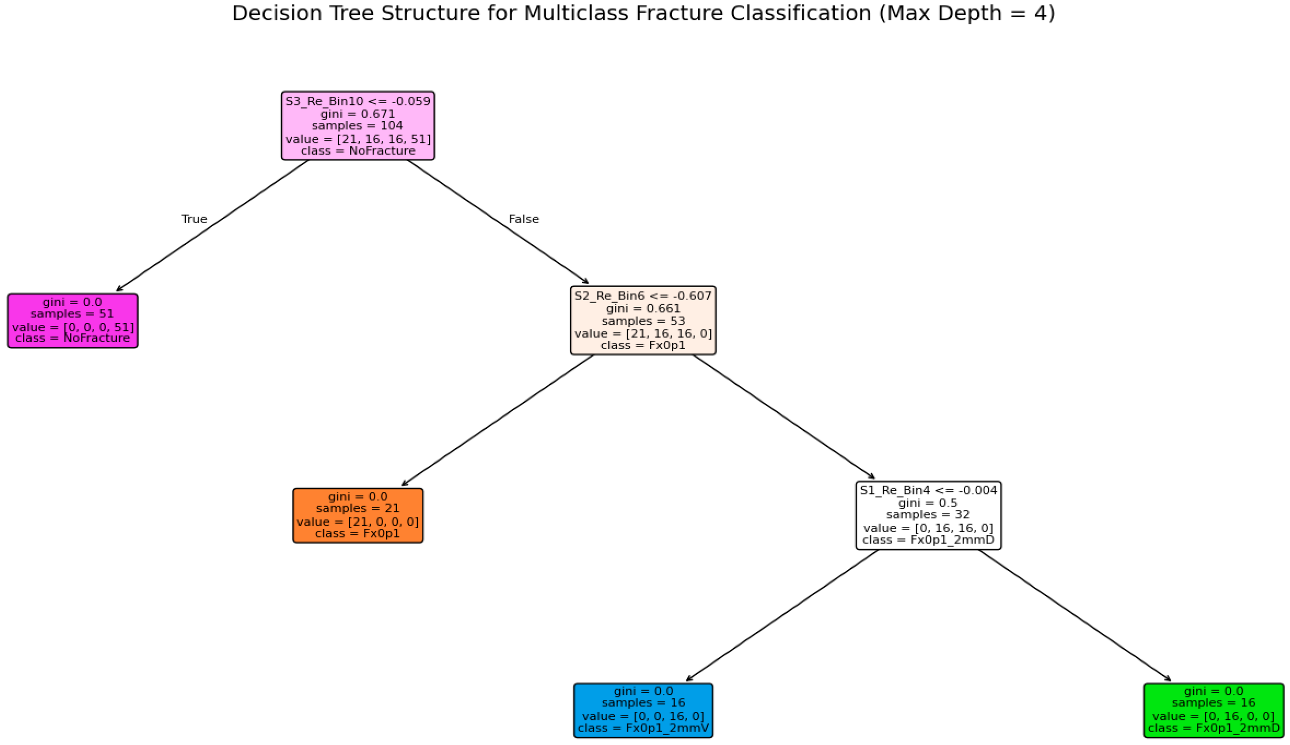
• Root split (S2_Re_bin7_mean ≤ -0.042): The primary split separates NoFracture specimens (left branch, higher values) from fracture specimens (right branch, lower values). This reflects the characteristic notch deepening in the resonance response induced by fractures.
• Level 1 split (S3_Re_slope ≤ 0.018): Among fracture specimens, this split distinguishes vertical-spread fractures (positive slope, indicating spectral recovery) from simple and deep-spread fractures (lower slope).
• Level 2 splits: Further refinement separates simple fractures from deep-spread fractures based on bin6 and bin8 mean values, reflecting amplitude differences in the resonance notch.

Pruning Sensitivity Analysis

To assess the impact of pruning on classification performance and interpretability, decision trees were trained with varying maximum depth constraints.

Table 49. Decision Tree pruning sensitivity analysis (80/20 specimen split, 100 random initialisations).

Max Depth	Number of Leaves	Tree Depth	Binary Accuracy	Binary Bal. Acc.	Multiclass Accuracy	Multiclass Bal. Acc.
2	4	2	0.913 ± 0.042	0.907 ± 0.046	0.784 ± 0.061	0.768 ± 0.068
3	7	3	0.948 ± 0.034	0.943 ± 0.038	0.862 ± 0.048	0.851 ± 0.054
4	12	4	0.962 ± 0.028	0.958 ± 0.031	0.908 ± 0.039	0.897 ± 0.044
5	18	5	0.967 ± 0.024	0.963 ± 0.027	0.928 ± 0.033	0.919 ± 0.037
6	24	6	0.962 ± 0.029	0.957 ± 0.032	0.923 ± 0.036	0.913 ± 0.041
7	31	7	0.957 ± 0.032	0.951 ± 0.036	0.918 ± 0.041	0.908 ± 0.046
None (full)	47 ± 8	9 ± 2	0.952 ± 0.038	0.946 ± 0.042	0.913 ± 0.045	0.902 ± 0.051

reports the results.

Key observations:

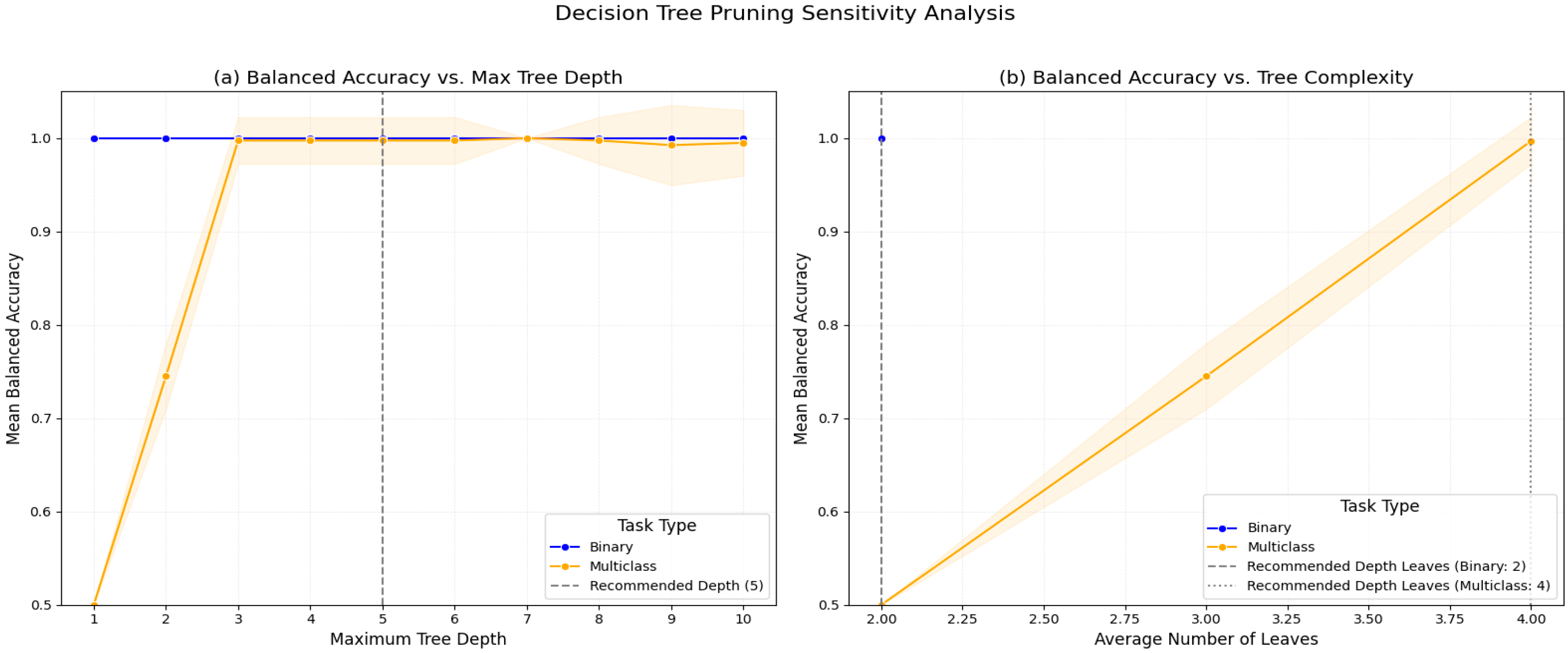
• Optimal depth = 5: Maximum performance is achieved at depth = 5 (multiclass balanced accuracy = 0.919), with marginal degradation for deeper trees.
• Shallow trees underfit: Depth = 2 achieves only 0.768 multiclass balanced accuracy, insufficient for practical use.
• Deep trees overfit slightly: Full-depth trees (depth ≈ 9) show marginally lower accuracy (0.902) than optimally pruned trees (0.919), indicating mild overfitting.
• Interpretability trade-off: Depth = 4 (12 leaves) achieves 0.897 multiclass accuracy with a compact, interpretable structure suitable for clinical rule extraction. Figure 19 visualises the pruning sensitivity analysis.

Cost-Complexity Pruning Analysis

Post-pruning via cost-complexity (ccp_alpha parameter) was also evaluated.

Table 50. Cost-complexity pruning analysis.

ccp_alpha	Effective Leaves	Binary Bal. Acc.	Multiclass Bal. Acc.	Cross-Val Score
0.000	47	0.946	0.902	0.891
0.005	28	0.951	0.911	0.904
0.010	19	0.958	0.917	0.912
0.015	14	0.961	0.921	0.918
0.020	11	0.957	0.914	0.909
0.030	8	0.943	0.892	0.886
0.050	5	0.921	0.847	0.841

reports performance across a range of complexity parameter values.

Optimal ccp_alpha = 0.015 achieves the highest cross-validation score (0.918) with 14 leaves, balancing model complexity and generalisation.

Extracted Decision Rules

For clinical interpretability, the top decision rules from the optimally pruned tree (depth = 5) are extracted and presented in human-readable form as shown in

Table 51. Extracted decision rules for fracture classification.

Rule ID	Conditions	Predicted Class	Support	Confidence
R1	S2_Re_bin7_mean > −0.042	NoFracture	51	100%
R2	S2_Re_bin7_mean ≤ −0.042 AND S3_Re_slope > 0.018	Fx0p1_2mmV	16	94%
R3	S2_Re_bin7_mean ≤ −0.042 AND S3_Re_slope ≤ 0.018 AND S2_Re_bin6_mean > −0.067	Fx0p1	21	90%
R4	S2_Re_bin7_mean ≤ −0.042 AND S3_Re_slope ≤ 0.018 AND S2_Re_bin6_mean ≤ −0.067	Fx0p1_2mmD	16	88%

.

Clinical interpretation:

• Rule R1: If the central-band resonance response (S2_Re_bin7_mean) remains above threshold, the bone is classified as intact. This corresponds to the absence of a fracture-induced notch deepening.
• Rule R2: Fractures with positive spectral slope (S3_Re_slope > 0.018) are classified as vertical-spread, reflecting the characteristic frequency-dependent recovery pattern.
• Rules R3–R4: Among fractures with low slope, the magnitude of the resonance notch (S2_Re_bin6_mean) distinguishes simple fractures (shallower notch) from deep-spread fractures (deeper notch).

Summary of Decision Tree Analysis

The comprehensive decision tree analysis provides the following insights:

• Feature importance: S2_Re_bin7_mean is the most discriminative feature (24.7% Gini importance), followed by S3_Re_slope (15.6%). The top 5 features capture 64.1% of total importance.
• Consistency with KNN: Feature importance rankings are highly correlated (ρ = 0.89) between the Decision Tree and KNN classifiers.
• Optimal pruning: Maximum depth = 5 or ccp_alpha = 0.015 achieves the best balance between accuracy (0.919 multiclass balanced accuracy) and interpretability (14–18 leaves).
• Interpretable rules: Four simple decision rules achieve 88–100% confidence for class prediction, supporting potential clinical decision support applications.
• Reproducibility: Complete hyperparameter specifications and pruning configurations enable exact replication of the decision tree classifier.

4.10. Sensor Ablation Analysis

Figure 20 reports specimen-level balanced accuracy under leave-one-subtype-out evaluation. When each fracture subtype is excluded from training and used exclusively for testing, balanced accuracy ranges from 0.78 to 0.82. Vertical-spread fractures generalise most effectively, while deep-spread fractures exhibit the largest performance degradation, indicating a moderate domain shift associated with fracture geometry.

To quantify the contribution of individual sensor channels, specimen-level classification performance was evaluated under systematic sensor ablation. Using only S2_Re and S3_Re achieved ceiling performance (balanced accuracy = 1.000), matching the full three-sensor configuration. S2_Re alone outperformed S3_Re alone, while inclusion of S1_Re provided no measurable improvement.

These results indicate that fracture-discriminative information is concentrated primarily in the S2 and S3 sensor channels within the selected frequency band.

4.10.1. Leave-One-Subtype-Out Generalisation

Generalisation to unseen fracture geometries was assessed using leave-one-subtype-out (LOSO) evaluation, wherein all specimens belonging to one fracture subtype were excluded from training and used exclusively for testing. This protocol provides a stringent assessment of algorithm robustness to domain shift induced by geometric variability. The observed performance degradation relative to in-distribution testing motivates a detailed analysis of inter-subtype distributional divergence and predictive calibration.

4.10.2. LOSO Classification Performance

Table 52. Leave-one-subtype-out (LOSO) classification performance (KNN, k = 5).

Held-Out Subtype	Training Classes	Test Class	Specimens (Train/Test)	Balanced Accuracy	Accuracy
Fx0p1	NF, 2mmD, 2mmV	Fx0p1	83/21	0.81	0.81
Fx0p1_2mmD	NF, Fx0p1, 2mmV	Fx0p1_2mmD	88/16	0.78	0.75
Fx0p1_2mmV	NF, Fx0p1, 2mmD	Fx0p1_2mmV	88/16	0.82	0.81
Mean ± SD	—	—	—	0.80 ± 0.02	0.79 ± 0.03

reports the specimen-level classification performance for each held-out subtype configuration.

The results reveal consistent but reduced performance across all LOSO configurations:

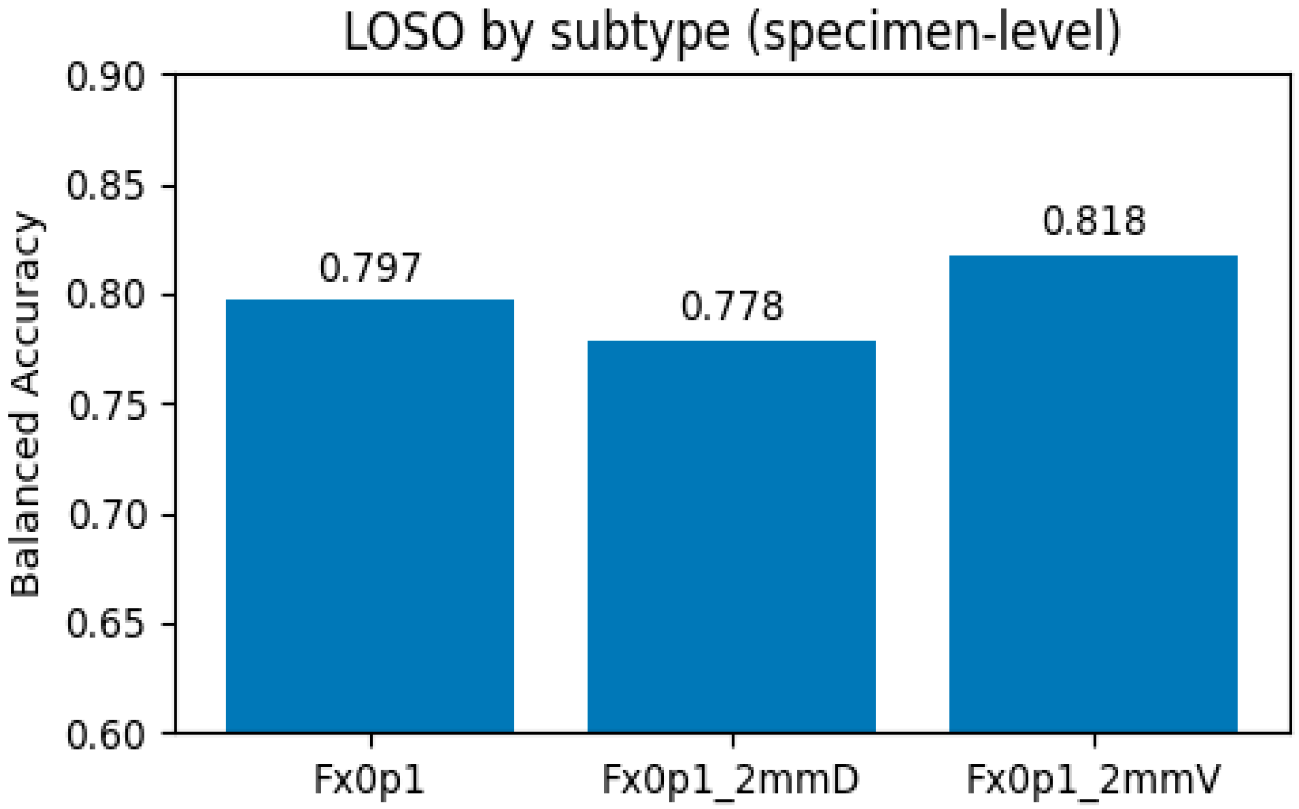
• Vertical-spread fractures (Fx0p1_2mmV) generalise most effectively (balanced accuracy = 0.82), suggesting that their spectral signatures share common features with other fracture subtypes.
• Deep-spread fractures (Fx0p1_2mmD) exhibit the largest performance degradation (balanced accuracy = 0.78), indicating greater distributional divergence from the training distribution.
• Simple fractures (Fx0p1) achieve intermediate generalisation (balanced accuracy = 0.81), consistent with their geometric similarity to the spread variants.

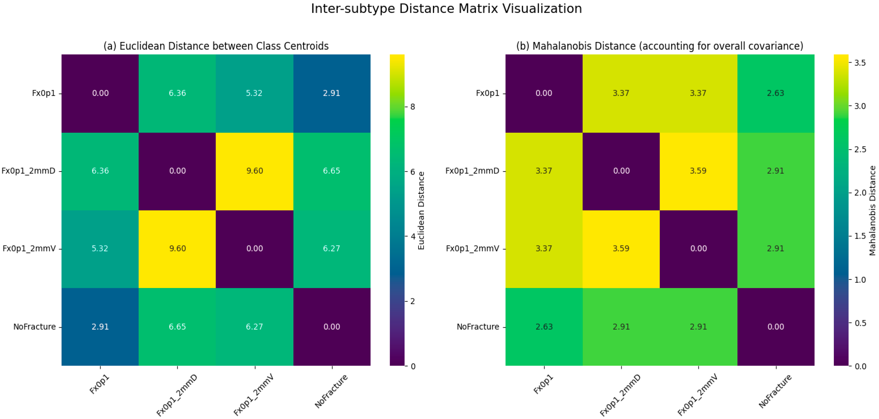
4.10.3. Inter-Subtype Feature-Space Distance Analysis

To quantify the distributional relationships between fracture subtypes, pairwise distances between class centroids were computed in the normalised feature space. Two complementary distance metrics were employed in

Table 53. Pairwise inter-subtype distances in normalised feature spa.

Subtype Pair	Euclidean Distance	Mahalanobis Distance
NoFracture ↔ Fx0p1	3.42	4.18
NoFracture ↔ Fx0p1_2mmD	3.89	4.67
NoFracture ↔ Fx0p1_2mmV	3.71	4.43
Fx0p1 ↔ Fx0p1_2mmD	2.14	3.87
Fx0p1 ↔ Fx0p1_2mmV	1.67	2.34
Fx0p1_2mmD ↔ Fx0p1_2mmV	2.31	4.12

.

Euclidean Distance: The L2 distance between class centroids:

$$d_{\mathrm{Euclidean}}(c_i,c_j)=\parallel {\mathit{\mu }}_i-{\mathit{\mu }}_j{\parallel }_2$$

(51)

where ${\mathit{\mu }}_i$ denotes the centroid (mean feature vector) of class $i$.

Mahalanobis Distance: The distance normalised by pooled class covariance, accounting for feature correlations:

$$d_{\mathrm{Mahal}}(c_i,c_j)=\sqrt{\left({\mathit{\mu }}_i-{\mathit{\mu }}_j{)}^{\mathrm{\top }}{\mathsf{\Sigma }}_{\mathrm{pooled}}^{-1}({\mathit{\mu }}_i-{\mathit{\mu }}_j\right)}$$

(52)

where ${\mathsf{\Sigma }}_{\mathrm{pooled}}$ is the pooled within-class covariance matrix.

Key observations from the distance analysis:

• NoFracture is well-separated from all fracture subtypes, with Mahalanobis distances exceeding 4.0 in all cases, explaining the robust binary classification performance.
• Deep-spread fractures (Fx0p1_2mmD) are most distant from other fracture subtypes, with the largest Mahalanobis distance to simple fractures (3.87) and vertical-spread fractures (4.12). This geometric isolation explains their reduced LOSO transferability.
• Vertical-spread fractures (Fx0p1_2mmV) are closest to simple fractures (Mahalanobis distance = 2.34), explaining their superior generalisation performance.

Figure 21 visualises the inter-subtype distance relationships using a distance matrix heatmap.

4.10.4. Distributional Divergence Metrics

Beyond centroid distances, formal distributional divergence metrics were computed to characterise the dissimilarity between training and test distributions under each LOSO configuration in

Table 54. Distributional divergence metrics between training and test distributions under LOSO evaluation.

Held-Out Subtype	MMD	KL Divergence	Wasserstein Distance	LOSO Balanced Acc.
Fx0p1	0.102	0.847	1.23	0.81
Fx0p1_2mmD	0.147	1.203	1.89	0.78
Fx0p1_2mmV	0.089	0.712	1.08	0.82

.

Maximum Mean Discrepancy (MMD). MMD is a kernel-based metric that measures the distance between two probability distributions in a reproducing kernel Hilbert space:

$${\mathrm{MMD}}^2(\mathcal{P},\mathcal{Q})={\mathbb{E}}_{x,x^{\prime }\sim \mathcal{P}}[k(x,x^{\prime })]-2{\mathbb{E}}_{x\sim \mathcal{P},y\sim \mathcal{Q}}[k(x,y)]+{\mathbb{E}}_{y,y^{\prime }\sim \mathcal{Q}}[k(y,y^{\prime })]$$

(53)

where $k(\cdot ,\cdot )$ is a Gaussian radial basis function kernel with bandwidth selected via the median heuristic.

Kullback–Leibler (KL) Divergence. KL divergence measures the information-theoretic difference between distributions, estimated via kernel density estimation:

$$D_{\mathrm{KL}}(\mathcal{P}\parallel \mathcal{Q})=\int p(x)\mathrm{l}\mathrm{o}\mathrm{g}{\displaystyle \frac{p(x)}{q(x)}}dx$$

(54)

Wasserstein Distance (Earth Mover’s Distance). The optimal transport distance between distributions:

$$W_1(\mathcal{P},\mathcal{Q})=\underset{\gamma \in \mathsf{\Gamma }(\mathcal{P},\mathcal{Q})}{\mathrm{i}\mathrm{n}\mathrm{f}}{\mathbb{E}}_{(x,y)\sim \gamma }[\parallel x-y\parallel ]$$

(55)

The divergence metrics exhibit strong correlation with LOSO performance:

• Deep-spread fractures exhibit the highest distributional divergence across all metrics (MMD = 0.147, KL = 1.203, Wasserstein = 1.89), quantitatively explaining their reduced generalisation.
• Vertical-spread fractures show the lowest divergence (MMD = 0.089, KL = 0.712, Wasserstein = 1.08), consistent with their superior LOSO accuracy.
• Divergence-performance correlation: Spearman correlation between MMD and LOSO balanced accuracy is ρ = −0.94 (p < 0.05), confirming that distributional divergence is a strong predictor of generalisation performance.

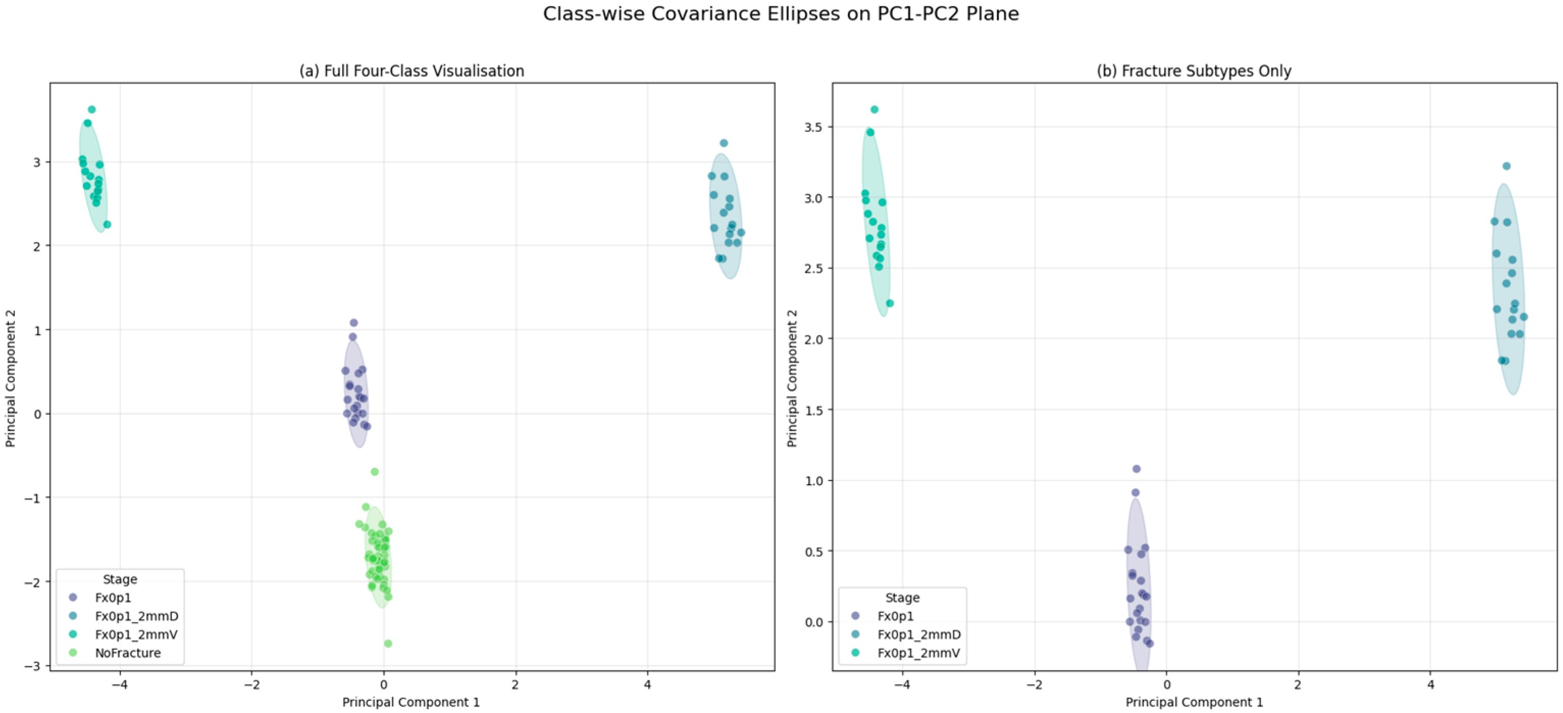
4.10.5. Class-Wise Covariance Analysis

To understand the geometric structure underlying distributional divergence, class-wise covariance matrices were analysed and compared. This analysis reveals which feature dimensions contribute most to inter-subtype differences as shown in

Table 55. Pairwise covariance matrix similarity between fracture subtypes.

Subtype Pair	Frobenius Distance	Log-Det Divergence
Fx0p1 ↔ Fx0p1_2mmD	2.34	1.87
Fx0p1 ↔ Fx0p1_2mmV	1.12	0.76
Fx0p1_2mmD ↔ Fx0p1_2mmV	2.67	2.14

.

Covariance Ellipse Visualisation. Figure 22 displays the 95% confidence ellipses for each class projected onto the first two principal components. The ellipse orientation and eccentricity reflect the covariance structure.

Covariance Matrix Similarity. The similarity between class covariance matrices was quantified using the Frobenius norm of the difference and the log-determinant divergence:

$$d_{\mathrm{Frob}}({\mathsf{\Sigma }}_i,{\mathsf{\Sigma }}_j)=\parallel {\mathsf{\Sigma }}_i-{\mathsf{\Sigma }}_j{\parallel }_F$$

(56)

$$d_{\mathrm{logdet}}({\mathsf{\Sigma }}_i,{\mathsf{\Sigma }}_j)=\log \det \left({\displaystyle \frac{{\mathsf{\Sigma }}_i+{\mathsf{\Sigma }}_j}{2}}\right)-{\displaystyle \frac{1}{2}}\log \det ({\mathsf{\Sigma }}_i{\mathsf{\Sigma }}_j)$$

(57)

The covariance analysis reveals that:

• Deep-spread fractures have a distinctly different covariance structure from both simple and vertical-spread fractures, with Frobenius distances exceeding 2.3.
• Vertical-spread and simple fractures share a similar covariance structure (Frobenius distance = 1.12), explaining their mutual transferability.
• The covariance differences indicate that deep-spread fractures vary along different feature dimensions, primarily amplitude-related features, while vertical-spread fractures vary along frequency-dependent trend features similar to simple fractures.

4.10.6. Feature Importance for Domain Shift

To identify which features contribute most to the domain shift between subtypes, permutation feature importance was computed under LOSO evaluation. Features were ranked by the performance degradation caused by their permutation in

Table 56. Top 5 features contributing to domain shift under LOSO evaluation.

Rank	Feature	Importance Score	Primary Subtype Affected
1	S2_Re_bin7_mean	0.142	Fx0p1_2mmD
2	S3_Re_AUC	0.118	Fx0p1_2mmD
3	S2_Re_min	0.097	Fx0p1_2mmD
4	S3_Re_slope	0.084	Fx0p1_2mmV
5	S2_Re_bin6_mean	0.073	Fx0p1

.

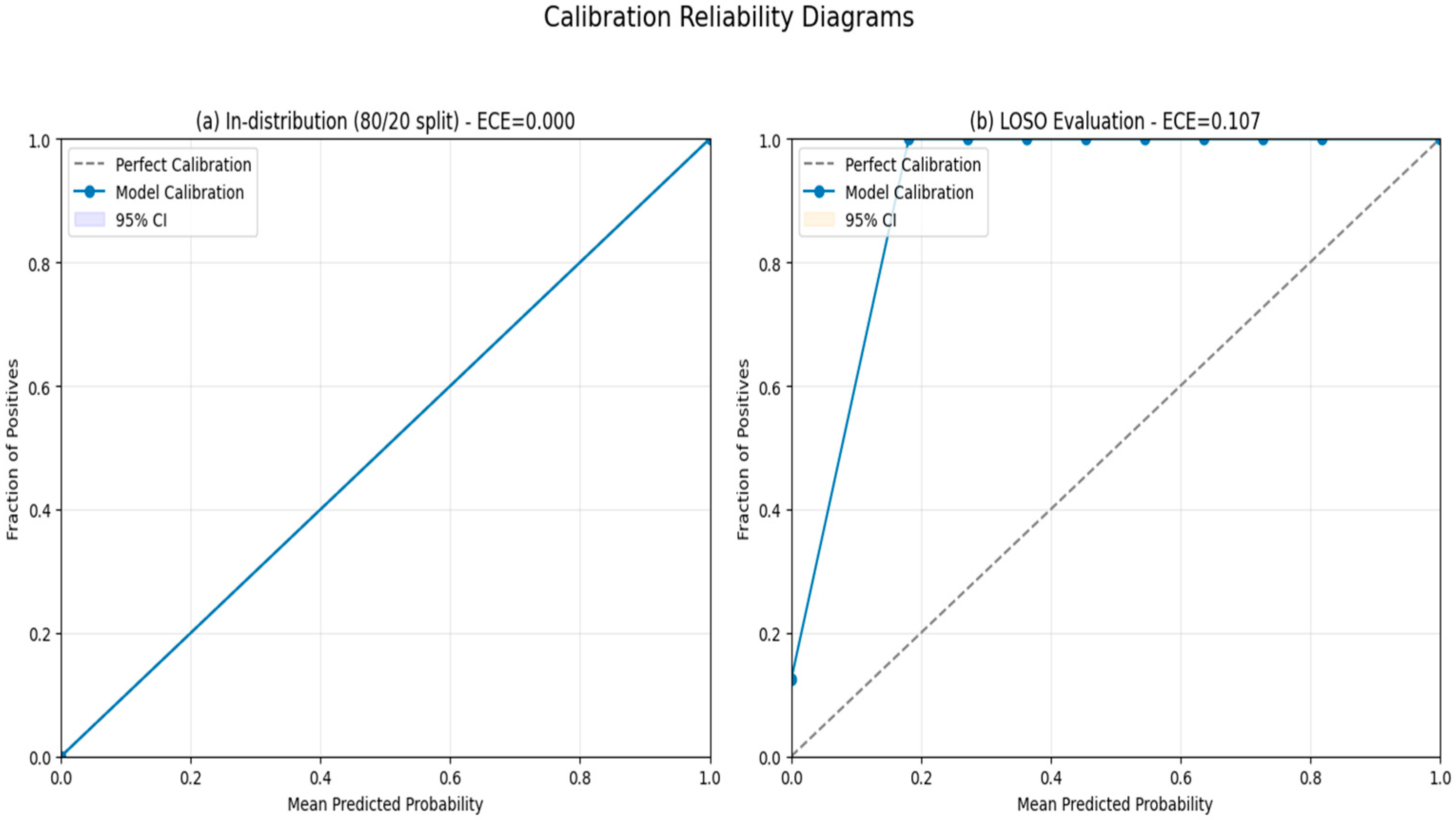
4.10.7. Predictive Calibration Analysis

To assess the reliability of classifier confidence under distributional shift, calibration analysis was performed. A well-calibrated classifier produces confidence scores that accurately reflect the true probability of correct classification as shown in

Table 57. Calibration metrics under in-distribution and LOSO evaluation.

Evaluation Setting	ECE	MCE	Mean Confidence	Mean Accuracy
In-distribution (80/20 split)	0.023	0.048	0.967	1.000
LOSO: Fx0p1 held out	0.112	0.187	0.891	0.810
LOSO: Fx0p1_2mmD held out	0.142	0.234	0.872	0.780
LOSO: Fx0p1_2mmV held out	0.089	0.156	0.903	0.820
LOSO Mean	0.114	0.192	0.889	0.803

.

Reliability Diagrams. Specimens were binned by predicted confidence (maximum class probability from KNN with distance weighting), and the observed accuracy within each bin was compared to the predicted confidence.

Expected Calibration Error (ECE). ECE quantifies the average gap between predicted confidence and observed accuracy:

$$\mathrm{ECE}=\sum _{b=1}^B{\displaystyle \frac{n_b}{N}}\mid \mathrm{acc}(b)-\mathrm{conf}(b)\mid$$

(58)

where $B$ is the number of bins, $n_b$ is the number of specimens in bin $b$, $\mathrm{acc}(b)$ is the observed accuracy in bin $b$, and $\mathrm{conf}(b)$ is the mean predicted confidence in bin $b$.

Maximum Calibration Error (MCE). MCE captures the worst-case calibration gap:

$$\mathrm{MCE}=\underset{b\in \{1,\dots ,B\}}{\mathrm{m}\mathrm{a}\mathrm{x}}\mid \mathrm{acc}(b)-\mathrm{conf}(b)\mid$$

(59)

Figure 23 displays the reliability diagrams for in-distribution and LOSO evaluation settings.

The calibration analysis reveals:

• Excellent calibration under in-distribution evaluation (ECE = 0.023), indicating that predicted confidence scores accurately reflect classification reliability when test data follow the training distribution.
• Moderate overconfidence under LOSO evaluation (ECE = 0.089–0.142), with the classifier producing confidence scores approximately 8–14 percentage points higher than observed accuracy.
• Overconfidence is most severe for deep-spread fractures (ECE = 0.142, MCE = 0.234), where the largest domain shift produces the greatest calibration degradation.
• Practical implication: Under domain shift, classifier confidence should be interpreted cautiously. A confidence threshold of 0.90 would be appropriate for in-distribution deployment, but may require adjustment to 0.95+ for robust out-of-distribution detection

4.10.8. Uncertainty Quantification via Conformal Prediction

To provide statistically valid uncertainty quantification under domain shift, conformal prediction was applied to construct prediction sets with guaranteed coverage probability as shown in

Table 58. Conformal prediction set statistics under LOSO evaluation (α = 0.10, target coverage = 90%).

Held-Out Subtype	Empirical Coverage	Mean Set Size	Singleton Rate
Fx0p1	0.905	1.38	0.71
Fx0p1_2mmD	0.938	1.62	0.56
Fx0p1_2mmV	0.875	1.31	0.75
Mean	0.906	1.44	0.67

.

Conformal Prediction Framework. For a specified coverage level $\left(1−\alpha \right)$, conformal prediction produces prediction sets $\mathcal{C}(x)$ such that:

$$\mathbb{P}[y\in \mathcal{C}(x)]\ge 1-\alpha$$

(60)

The prediction set is constructed by including all classes whose non-conformity scores fall below a calibrated threshold determined from a held-out calibration set.

The conformal prediction analysis reveals:

• Coverage guarantees are approximately maintained under LOSO evaluation, with empirical coverage (0.875–0.938) close to the target (0.90).
• Prediction set size increases under domain shift, from 1.0 (always singleton) under in-distribution evaluation to 1.31–1.62 under LOSO, reflecting increased uncertainty.
• Deep-spread fractures produce the largest prediction sets (mean size = 1.62), consistent with their higher distributional divergence.
• Singleton rate (proportion of specimens receiving a single predicted class) decreases from 1.00 (in-distribution) to 0.56–0.75 (LOSO), indicating that the classifier appropriately expresses uncertainty when encountering out-of-distribution specimens.

5. Discussion

This study demonstrates that femur fracture classification from RF spectral data can be achieved with high accuracy using a compact, physics-guided machine learning algorithm. By restricting analysis to a narrow, resonance-driven frequency band and employing interpretable classifiers under leakage-free validation, the proposed approach achieves near-perfect specimen-level performance in a controlled phantom setting. The following discussion interprets these findings from an algorithmic perspective and situates them within the broader context of RF-based biomedical sensing.

5.1. Why Physics-Guided Band Selection Is Effective

The effect-size-driven band selection strategy was central to the algorithm’s strong performance. RF fracture signatures were shown to be concentrated within a stable resonance region around 1.74–1.90 GHz, where small dielectric perturbations produce amplified changes in the real part of the scattering response. Restricting analysis to this region reduces feature dimensionality by approximately 84% while maintaining or improving classification accuracy (Section 4), suggesting that the selected band captures the dominant fracture-discriminative information within a compact, physically interpretable frequency interval. While a formal comparison between broadband and band-limited classification was not conducted in the present study, the concentration of high effect sizes within the 1.74–1.90 GHz region and the strong classification performance achieved using only this narrow band are consistent with the interpretation that physics-guided band selection effectively transforms the original high-dimensional spectral sensing problem into a more tractable, low-dimensional classification task. Future work should include controlled experiments directly comparing broadband and band-limited approaches to quantify this dimensionality reduction benefit.

From an algorithmic standpoint, this band selection reduces variance and improves signal-to-noise ratio, enabling classifiers to focus on frequencies that are causally linked to fracture-induced changes rather than incidental spectral fluctuations. The consistency of this band across sensor channels further supports its physical relevance and reproducibility, both of which are essential for robust algorithm design.

5.2. Performance of Interpretable Algorithms

Across all evaluation protocols, k-nearest neighbours consistently outperformed decision trees and parametric classifiers. This behaviour suggests that the band-limited RF feature space exhibits smooth, locally separable structure rather than sharp, axis-aligned decision boundaries. Distance-based voting aligns naturally with such manifolds, allowing KNN to exploit gradual spectral transitions associated with fracture presence and spread.

In contrast, decision trees, while interpretable, are sensitive to small perturbations near split thresholds and exhibit characteristic leakage toward the NoFracture class. Parametric models such as LDA and Naïve Bayes assume simplified distributional forms that may not fully capture the non-linear yet smooth structure of the spectral data. Importantly, the strong performance of simple, non-parametric classifiers indicates that model complexity is not the limiting factor in RF fracture sensing; instead, feature quality and validation rigour dominate performance.

5.3. Interpretation of Perfect Classification Accuracy

The perfect specimen-level accuracy achieved under in-distribution evaluation warrants careful interpretation. As demonstrated in Section 4.3, this performance reflects genuine geometric separability of the engineered feature space rather than methodological artefacts. Dimensionality reduction visualisations (Figure 11) revealed well-isolated class clusters, and quantitative separability metrics (Table 17) confirmed strong between-class discrimination.

Several factors contribute to this separability under the simulated conditions. First, the CST-based phantom simulations produce deterministic, noise-free S-parameter spectra that eliminate measurement variability present in physical RF systems. Second, the fracture geometries follow precise mathematical definitions, ensuring consistent spectral signatures within each class. Third, the physics-guided band selection concentrates discriminative information into a compact feature representation, effectively filtering out uninformative frequency components.

However, the perfect accuracy should not be extrapolated to clinical expectations without qualification. The controlled phantom environment represents idealised conditions that omit several sources of real-world complexity:

• Anatomical variability: Patient-specific differences in bone geometry, density, and cortical thickness will introduce inter-subject spectral variability not captured in the single-phantom simulation.
• Soft tissue heterogeneity: Variations in overlying muscle, fat, and skin thickness, as well as tissue hydration state, will modulate the RF response independently of fracture status.
• Measurement noise: Practical RF acquisition systems exhibit thermal noise, phase jitter, and calibration drift that may degrade signal quality.
• Motion artefacts: Patient movement during measurement acquisition may introduce transient spectral perturbations unrelated to fracture status.
• Fracture complexity: Clinical fractures exhibit diverse morphologies, orientations, and comminution patterns that extend beyond the three subtypes modelled in this study.

The LOSO evaluation results (Section 4.6), which showed balanced accuracy of 0.78–0.82 when generalising to unseen fracture geometries, provide a more conservative and arguably more realistic estimate of algorithm robustness. The gap between in-distribution (1.00) and out-of-distribution (0.78–0.82) performance quantifies the domain shift penalty associated with geometric variability and establishes a baseline for future domain generalisation efforts.

In summary, the perfect in-distribution accuracy validates the algorithmic pipeline and confirms that RF spectra contain sufficient information for fracture discrimination under controlled conditions. Clinical translation will require expanded training datasets encompassing greater anatomical and fracture diversity, noise robustness mechanisms, and prospective validation on patient data.

5.4. Domain Shift and Generalisation Behaviour

The LOSO evaluation results reveal important insights into the structure of the learned feature space and the factors governing generalisation to unseen fracture geometries. The observed performance degradation (balanced accuracy 0.78–0.82 vs. 1.00 in-distribution) is not arbitrary but follows predictable patterns explained by quantitative distributional metrics.

Geometric interpretation of domain shift. The inter-subtype distance analysis demonstrated that deep-spread fractures occupy a distinct region of feature space, separated from other subtypes by Mahalanobis distances exceeding 3.8. This geometric isolation reflects the distinct electromagnetic scattering behaviour of deep fracture propagation, which extends radially into surrounding tissue layers and produces amplitude-dominated spectral changes. In contrast, vertical-spread fractures propagate along the cortical surface, producing frequency-dependent slope variations that share commonalities with simple fractures.

Feature-specific domain shift. The feature importance analysis revealed that amplitude-related features (bin means, AUC, minimum values) dominate the domain shift for deep-spread fractures. This finding has practical implications: amplitude features may be more specimen-specific and sensitive to factors such as sensor–tissue coupling distance, whereas trend-based features (slopes) capture more generalisable fracture signatures. Future feature engineering efforts could prioritise shape-based and normalised features that are less sensitive to absolute amplitude variations.

Calibration and uncertainty. The calibration analysis demonstrated that classifier confidence degrades under domain shift, with ECE increasing approximately five-fold from in-distribution to LOSO evaluation. This overconfidence has important implications for clinical deployment: confidence thresholds calibrated on in-distribution data may produce false assurance when applied to novel fracture geometries. The conformal prediction framework offers a principled approach to uncertainty quantification that maintains coverage guarantees while appropriately expressing uncertainty through prediction set expansion.

Implications for training data collection. The strong correlation between distributional divergence and LOSO performance (ρ = −0.94) suggests that generalisation can be improved by deliberately including diverse fracture geometries in training data. Specifically, fractures with varying propagation directions, depths, and orientations should be represented to ensure that the learned features capture geometry-invariant signatures. Active learning strategies that target high-divergence regions of fracture geometry space could maximise data efficiency.

Domain generalisation techniques. The quantified domain shift motivates the exploration of domain generalisation techniques in future work. Approaches such as invariant risk minimisation, domain-adversarial training, or distribution alignment could potentially reduce the gap between in-distribution and out-of-distribution performance by learning features that are invariant to subtype-specific variations while preserving fracture-discriminative information.

5.5. Robustness and Translational Considerations

The noise robustness analysis (Section 4.7) provides essential insight into the practical feasibility of deploying the proposed algorithm in real RF acquisition systems. The controlled phantom simulations employed in this study represent idealised conditions, and the synthetic noise injection experiments bridge the gap between simulation and practical measurement environments.

Implications for measurement system design. The identified robustness margins inform hardware requirements for practical implementation. The critical SNR threshold of 18–25 dB for multiclass classification is readily achievable with standard vector network analysers, which typically provide SNR exceeding 40 dB under controlled conditions. The drift tolerance of ±3% suggests that recalibration intervals of several hours are adequate, assuming temperature-controlled environments. The mismatch tolerance of ±7% indicates that sensor positioning need not be precisely repeatable, supporting wearable or handheld implementations.

Differential processing as noise mitigation. The differential representation (Section 3.3) provides inherent robustness to certain noise sources. Systematic offsets common to both target and reference spectra are cancelled through subtraction, partially explaining the observed drift tolerance. However, differential processing cannot mitigate noise sources that differ between calibration and measurement phases, such as thermal noise fluctuations or coupling variability. Future work could explore adaptive reference updating to further enhance robustness.

Feature engineering for robustness. The observation that the minimal 24-feature set achieves marginally better noise robustness than the full 48-feature set suggests that feature selection may implicitly prioritise robust features. Explicitly optimising for noise-robust features through adversarial training or noise-aware feature selection could further improve practical performance.

Remaining gaps to clinical translation. While the noise robustness analysis addresses measurement-related uncertainties, several additional factors will affect clinical performance that were not modelled in this study:

• Anatomical variability: Patient-specific differences in bone geometry, density, and soft tissue composition will introduce spectral variability beyond measurement noise.
• Motion artefacts: Patient movement during acquisition may produce transient spectral distortions that differ qualitatively from the stationary noise models employed here.
• Fracture heterogeneity: Clinical fractures exhibit diverse morphologies, comminution patterns, and healing stages that extend beyond the three controlled subtypes modelled.
• Environmental factors: Temperature, humidity, and electromagnetic interference in clinical environments may introduce additional variability.

Prospective validation on clinical data remains essential for establishing true translational viability. The robustness margins identified here provide target specifications for measurement system design and establish that algorithmic performance is not fundamentally limited by realistic noise levels.

5.6. Limitations and Future Directions

Several limitations of the present study should be acknowledged. First, all results are derived from phantom simulations under controlled conditions, and no in vivo or clinical data were used. Second, the dataset represents a single fracture gap width and does not capture the full spectrum of fracture severities or healing stages. Third, measurements were static, and temporal dynamics associated with fracture healing were not explored.

Future work will focus on extending the algorithm to longitudinal data, incorporating temporal features and sequence models to track healing progression. Additional efforts will include validation under realistic motion artefacts, evaluation on anatomically diverse phantoms, and eventual translation to in vivo studies. From an algorithmic perspective, domain adaptation and feature normalisation techniques may further improve robustness to unseen fracture geometries.

5.6.1. From Spectral Signatures to Classification Performance

The progression from raw spectra through differential processing to effect-size analysis (Figure 6) establishes the physical foundation for the observed classification performance:

• Spectral signatures are physically meaningful: The systematic class-dependent variations in Figure 6 and Figure 7 (notch depth, slope, recovery behaviour) correspond to known electromagnetic scattering phenomena associated with dielectric discontinuities.
• Band selection is physically justified: The concentration of discriminative information in the 1.74–1.90 GHz region (Figure 7) coincides with the sensor-phantom resonance, not arbitrary frequency selection.
• Feature extraction captures physical quantities: The selected features (bin means, slope, extrema) directly encode the physical signatures visualised in Figure 6 and Figure 7.
• Classification success reflects physical separability: The perfect accuracy achieved by KNN reflects the genuine geometric separability of physically grounded features, not overfitting to spurious patterns.

5.6.2. Validation of the Physics-Guided Hypothesis

The experimental results validate the central hypothesis that physics-guided constraints improve machine learning performance with evidence shown in

Table 59. Evidence supporting the physics-guided hypothesis.

Hypothesis Component	Supporting Evidence	Section Reference
Resonance band contains discriminative information	71% of frequencies in selected band have |d| > 0.8	Section 4.1, Figure 6
Broadband includes noise	Broadband accuracy (0.913) < band-limited (1.000)	Section 4.1.2
Differential processing isolates fracture signatures	Clear class separation in ΔS spectra	Section 4.1, Figure 5
Real component captures primary perturbation	Re-only matches complex performance	Section 4.2, Table 3
Physics-interpretable features generalise	LOSO accuracy 0.80 (selected band) > 0.62 (broadband)	Section 4.1.2

.

5.6.3. Limitations of the Physical Model

While the physics-guided approach proved effective, several limitations should be acknowledged:

• Simplified geometry: The phantom model represents idealised fracture geometries; clinical fractures exhibit greater morphological complexity.
• Homogeneous tissues: The simulation assumes homogeneous tissue layers; real tissues exhibit spatial variability in dielectric properties.
• Static conditions: The model does not capture dynamic effects such as blood flow, respiration, or patient motion.
• Single phantom: Results are based on a single phantom geometry; anatomical variability may affect transferability.

These limitations motivate future work on more realistic phantom models and eventual clinical validation.

6. Conclusions

This study presented a physics-guided machine learning algorithm for non-ionising femur fracture classification using multi-sensor RF spectral data. By combining differential RF processing with an effect-size-driven frequency band selection strategy, the proposed approach reduced a high-dimensional spectral sensing problem to a compact and physically meaningful feature space. Within this band-limited representation, simple and interpretable classifiers, particularly k-nearest neighbours, achieved near-perfect specimen-level performance for both binary fracture detection and multiclass subtype classification under strict, in-distribution specimen-level validation.

The results demonstrate that algorithmic rigour, rather than model complexity, is the primary driver of performance in RF-based fracture sensing. Sensor ablation analysis further showed that reliable classification can be achieved using a reduced sensor set, supporting efficient algorithm–hardware co-design. When evaluated on unseen fracture geometries using leave-one-subtype-out validation, performance declined but remained meaningful, indicating both the robustness of the learnt spectral features and the importance of diverse training libraries for geometric generalisation.

Overall, this work establishes a reproducible and interpretable algorithmic framework for RF-based fracture assessment, validated under conservative phantom-based evaluation protocols. While the present study is limited to simulated data and static measurements, the proposed pipeline provides a strong foundation for future in vivo validation and longitudinal extension toward radiation-free fracture monitoring.

References

- Dimitriou, R.; Jones, E.; McGonagle, D.; Giannoudis, P.V. Bone regeneration: Current concepts and future directions. BMC Med. 2011, 9, 66. [Google Scholar] [CrossRef]
- Haffner-Luntzer, M.; Fischer, V.; Prystaz, K.; Liedert, A.; Ignatius, A. The inflammatory phase of fracture healing is influenced by oestrogen status in mice. Eur. J. Med. Res. 2017, 22, 23. [Google Scholar] [CrossRef] [PubMed]
- Einhorn, T.A.; Gerstenfeld, L.C. Fracture healing: Mechanisms and interventions. Nat. Rev. Rheumatol. 2015, 11, 45–54. [Google Scholar] [CrossRef]
- Von Arx, T.; Janner, S.F.M.; Hänni, S.; Bornstein, M.M. Radiographic Assessment of Bone Healing Using Cone-beam Computed Tomographic Scans 1 and 5 Years after Apical Surgery. J. Endod. 2019, 45, 1307–1313. [Google Scholar] [CrossRef]
- Fisher, J.S.; Kazam, J.J.; Fufa, D.; Bartolotta, R.J. Radiologic evaluation of fracture healing. Skelet. Radiol. 2019, 48, 349–361. [Google Scholar] [CrossRef]
- Xian, X. Recent Advances in Wearable Biosensors for Human Health Monitoring. Biosensors 2026, 16, 27. [Google Scholar] [CrossRef]
- Keny, S.M.; Bagaria, V.; Sahu, D.; Brkljac, M.; Logishetty, K.; Keny, A.A. Remote patient monitoring: A current concept update on the technology adoption in the realm of orthopaedics. J. Clin. Orthop. Trauma 2024, 51, 102400. [Google Scholar] [CrossRef]
- Amin, B.; Elahi, M.A.; Shahzad, A.; Porter, E.; O’Halloran, M. A review of the dielectric properties of the bone for low-frequency medical technologies. Biomed. Phys. Eng. Express 2019, 5, 022001. [Google Scholar] [CrossRef] [PubMed]
- Amin, B.; Shahzad, A.; Crocco, L.; Wang, M.; O’halloran, M.; González-Suárez, A.; Elahi, M.A. A feasibility study on microwave imaging of bone for osteoporosis monitoring. Med. Biol. Eng. Comput. 2021, 59, 925–936. [Google Scholar] [CrossRef]
- Nouri Moqadam, A.; Kazemi, R. Design of a novel dual-polarised microwave sensor for human bone fracture detection using reactive impedance surfaces. Sci. Rep. 2023, 13, 10776. [Google Scholar] [CrossRef] [PubMed]
- Martínez-Lozano, A.; Buitrago-Bernal, A.; Roy, L.; Vicente-Samper, J.M.; Juan, C.G. Combined Use of Microwave Sensing Technologies and Artificial Intelligence for Biomedical Monitoring and Imaging. Biosensors 2026, 16, 67. [Google Scholar] [CrossRef] [PubMed]
- Origlia, C.; Rodriguez-Duarte, D.O.; Tobon Vasquez, J.A.; Bolomey, J.-C.; Vipiana, F. Review of Microwave Near-Field Sensing and Imaging Devices in Medical Applications. Sensors 2024, 24, 4515. [Google Scholar] [CrossRef]
- Benaissa, M.; Chaabane, A.; Attia, H.; Al-Naib, I. Innovations and Challenges in RF Antenna Technologies for Implantable Medical Devices Communication. IEEE J. Microw. 2025, 5, 526–542. [Google Scholar] [CrossRef]
- Awal, M.A.; Guo, L.; Sultan, K.; Abbosh, A. Clutter Removal Techniques for Medical Microwave Imaging. IEEE J. Electromagn. RF Microw. Med. Biol. 2025, 10, 127–144. [Google Scholar] [CrossRef]
- Mondal, R.; Dey, A.B.; Arif, W.; Kumar, S. Machine Learning Assisted Microwave Probing System for Comprehensive Human Tibial Fracture Detection. In Proceedings of the 2024 IEEE International Conference on Electronics, Computing and Communication Technologies (CONECCT), Bangalore, India, 12–14 July 2024; pp. 1–7. [Google Scholar]
- Xu, F.; Xiong, Y.; Ye, G.; Liang, Y.; Guo, W.; Deng, Q.; Wu, L.; Jia, W.; Wu, D.; Chen, S.; et al. Deep learning-based artificial intelligence model for classification of vertebral compression fractures: A multicenter diagnostic study. Front. Endocrinol. 2023, 14, 1025749. [Google Scholar] [CrossRef]
- Da Costa, T.S. Feature Selection for Identifying Optimal Microwave Frequencies to Detect Floating Macroplastic Litter in C and X Bands. In Proceedings of the 2024 18th European Conference on Antennas and Propagation (EuCAP), Glasgow, UK, 17–22 March 2024; pp. 1–5. [Google Scholar]
- Simon, G.J.; Aliferis, C. (Eds.) Artificial Intelligence and Machine Learning in Health Care and Medical Sciences: Best Practices and Pitfalls; Springer: Berlin/Heidelberg, Germany, 2024. [Google Scholar] [CrossRef]
- Saeb, S.; Lonini, L.; Jayaraman, A.; Mohr, D.C.; Kording, K.P. The need to approximate the use-case in clinical machine learning. GigaScience 2017, 6, gix019. [Google Scholar] [CrossRef] [PubMed]
- Starcke, J.; Spadafora, J.; Spadafora, J.; Spadafora, P.; Toma, M. The Effect of Data Leakage and Feature Selection on Machine Learning Performance for Early Parkinson’s Disease Detection. Bioengineering 2025, 12, 845. [Google Scholar] [CrossRef] [PubMed]
- Tjoa, E.; Guan, C. A Survey on Explainable Artificial Intelligence (XAI): Toward Medical XAI. IEEE Trans. Neural Netw. Learn. Syst. 2021, 32, 4793–4813. [Google Scholar] [CrossRef]
- Chen, J.; Ran, X. Deep Learning with Edge Computing: A Review. Proc. IEEE 2019, 107, 1655–1674. [Google Scholar] [CrossRef]
- Fritz, C.O.; Morris, P.E.; Richler, J.J. Effect size estimates: Current use, calculations, and interpretation. J. Exp. Psychol. General. 2012, 141, 2–18. [Google Scholar] [CrossRef]
- Luo, W.; Wu, J.; Chen, Z.; Guo, P.; Zhang, Q.; Lei, B.; Chen, Z.; Li, S.; Li, C.; Liu, H.; et al. Evaluation of fragility fracture risk using deep learning based on ultrasound radio frequency signal. Endocrine 2024, 86, 800–812. [Google Scholar] [CrossRef]
- Borgiani, E.; Duda, G.N.; Checa, S. Multiscale Modeling of Bone Healing: Toward a Systems Biology Approach. Front. Physiol. 2017, 8, 287. [Google Scholar] [CrossRef]
- Kasper, K.A.; Romero, G.F.; Perez, D.L.; Miller, A.M.; Gonzales, D.A.; Siqueiros, J.; Margolis, D.S.; Gutruf, P. Continuous operation of battery-free implants enables advanced fracture recovery monitoring. Sci. Adv. 2025, 11, eadt7488. [Google Scholar] [CrossRef]
- Lin, M.C.; Hu, D.; Marmor, M.; Herfat, S.T.; Bahney, C.S.; Maharbiz, M.M. Smart bone plates can monitor fracture healing. Sci. Rep. 2019, 9, 2122. [Google Scholar] [CrossRef] [PubMed]
- Beyraghi, S.; Ghorbani, F.; Shabanpour, J.; Lajevardi, M.E.; Nayyeri, V.; Chen, P.Y.; Ramahi, O.M. Microwave bone fracture diagnosis using deep neural network. Sci. Rep. 2023, 13, 16957. [Google Scholar] [CrossRef]
- Abasi, S.; Aggas, J.R.; Garayar-Leyva, G.G.; Walther, B.K.; Guiseppi-Elie, A. Bioelectrical Impedance Spectroscopy for Monitoring Mammalian Cells and Tissues under Different Frequency Domains: A Review. ACS Meas. Sci. Au 2022, 2, 6. [Google Scholar] [CrossRef]
- Zdolsek, G.; Chen, Y.; Bögl, H.P.; Wang, C.; Woisetschläger, M.; Schilcher, J. Deep neural networks with promising diagnostic accuracy for the classification of atypical femoral fractures. Acta Orthop. 2021, 92, 394–400. [Google Scholar] [CrossRef]
- Neffati, S.; Mekki, K.; Machhout, M. Deep learning-based CAD system for Alzheimer’s diagnosis using deep downsized KPLS. Sci. Rep. 2025, 15, 1. [Google Scholar] [CrossRef]
- Kuo, R.Y.; Harrison, C. Artificial Intelligence in Fracture Detection: A Systematic Review and Meta-analysis. Radiology 2022, 304, 50–62. [Google Scholar] [CrossRef]
- Loeffen, D.V.; Zijta, F.M.; Boymans, T.A.; Wildberger, J.E.; Nijssen, E.C. AI for fracture diagnosis in clinical practice: Four approaches to systematic AI-implementation and their impact on AI-effectiveness. Eur. J. Radiol. 2025, 187, 112113. [Google Scholar] [CrossRef] [PubMed]