A Comparative Analysis of U-Net Architectures with Dimensionality Reduction for Agricultural Crop Classification Using Hyperspectral Data

Abstract

The inherent high dimensionality of hyperspectral imagery presents both opportunities and challenges for agricultural crop classification. This study offers a rigorous comparative evaluation of three U-Net-based architectures, i.e., U-Net, U-Net++, and Atrous U-Net, applied to EnMAP hyperspectral data over the heterogeneous agricultural region of Lake Vegoritida, Greece. To address the spectral redundancy, we integrated multiple dimensionality-reduction strategies, including Linear Discriminant Analysis, SHAP-based model-driven feature selection, and unsupervised clustering approaches. Results reveal that model performance is contingent on (a) the network’s architecture and (b) the features’ space provided by band selection. While U-Net++ consistently excels when the full spectrum or ACS-derived subsets are employed, standard U-Net achieves great performance under LDA reduction, and Atrous U-Net benefits from SHAP-driven compact representations. Importantly, band selection methods such as ACS and SHAP substantially reduce spectral dimensionality without sacrificing accuracy, with the U-Net++–ACS configuration delivering the highest F1-score (0.77). These findings demonstrate that effective hyperspectral crop classification requires a joint optimization of architecture and spectral representation, underscoring the potential of compact, interpretable pipelines for scalable and operational precision agriculture.

1. Introduction

Crop mapping, the process of identifying and monitoring crop types and their spatial distribution, has become a cornerstone of modern agriculture. Crop mapping using remote sensing data plays a crucial role in enhancing food security, particularly in the face of climate change and population growth. By providing accurate and timely information on crop health and yield predictions, farmers can make informed decisions regarding resource allocation and crop rotation strategies, ultimately leading to increased productivity and sustainability [1,2,3,4]. Hyperspectral remote sensing (HRS) has undergone significant developments and achieved numerous milestones in the field of crop monitoring and mapping over the past several decades. Initially focused on mineral exploration in the 1960s, its application to agriculture gained momentum in the 1980s and 1990s with projects like LACIE and AgRISTARS, which demonstrated the potential of remote sensing for crop monitoring [5]. The transition from multispectral to hyperspectral sensors marked a significant milestone, allowing for the capture of hundreds of contiguous spectral bands. Hyperspectral data from the Hyperion sensor onboard EO-1 were evaluated for crop classification in northeastern Greece, demonstrating higher accuracy than Landsat 5 TM data. The inclusion of Hyperion’s SWIR bands enhanced crop discrimination, highlighting the potential of hyperspectral imaging for precision agriculture [6]. This advancement enabled more detailed analysis of crop characteristics and environmental conditions [7]. The ability to distinguish between different crop types and detect stress factors like drought and nutrient deficiencies has been a major achievement of HRS, enhancing precision agriculture practices [8,9]. Thus, hyperspectral data embody considerable potential for the accurate and efficient representation of agricultural landscapes, which is vital for the advancement of sustainable agricultural practices, resource governance, and prudent decision-making.

The high dimensionality of hyperspectral data presents several challenges that complicate its analysis and application. One primary issue is the “curse of dimensionality,” which refers to the exponential increase in data volume as the number of spectral bands increases, leading to computational inefficiencies and storage burdens [10,11]. This high dimensionality often results in highly correlated information across bands, which can degrade classification accuracy due to redundancy and noise [12]. Additionally, the vast number of spectral bands compared with the limited number of training samples can lead to overfitting in machine learning models, reducing their generalization capability [13].

The complexity of hyperspectral data also includes challenges such as spectral mixing and changes, which complicate target detection and classification tasks [14]. To address these issues, various dimensionality reduction (DR) techniques have been developed. These include methods like principal component analysis (PCA) and partial least squares (PLS), which aim to reduce the number of spectral bands while retaining essential information for classification [15]. Advanced methods such as semi-supervised spatial spectral regularized manifold local scaling cut (S3RMLSC) and locally adaptive dimensionality reduction metric learning (LADRml) have been proposed to exploit both spectral and spatial information, improving classification accuracy by preserving the data’s original distribution and handling complex data structures [16,17]. Furthermore, methods like the improved spatial-spectral weight manifold embedding (ISS-WME) and local and global sparse representation (LGDRSR) integrate spatial and spectral information to enhance the discriminative performance of hyperspectral images [18,19]. These approaches demonstrate the ongoing efforts to mitigate the challenges posed by high dimensionality in hyperspectral data, aiming to improve processing efficiency and classification outcomes.

In recent years, deep learning models, particularly convolutional neural networks (CNNs), have become a cornerstone in the field of remote sensing, offering significant advancements in various applications such as object detection, image classification, and change detection. CNNs excel in automatically extracting and representing features from remote sensing imagery, which is crucial for various applications [20,21]. The adaptability of CNNs to different tasks is evident in their application to land cover mapping, where they have been extensively used to classify and segment images without the need for manual feature extraction [22]. Moreover, CNNs have been employed to address challenges in remote sensing, such as color consistency, where they help in maintaining texture details while adjusting for color discrepancies across images [23]. In change detection, CNNs like the SSCFNet have been developed to enhance the extraction of both high-level and low-level semantic features, improving the detection of changes in remote sensing images [24]. The versatility of CNNs is further demonstrated in multimodal data classification, where frameworks like CCR-Net integrate data from different sources, such as hyperspectral and LiDAR, to improve classification accuracy [25]. Despite their success, deploying CNNs in resource-constrained environments, such as spaceborne applications, poses challenges due to the computational demands. Solutions like the automatic deployment of CNNs on FPGAs have been proposed to optimize performance while minimizing power consumption [26]. Additionally, innovative architectures like the multi-granularity fusion network (MGFN) and Siamese CNNs have been developed to enhance scene classification by capturing deep spatial features and addressing the limitations of small-scale datasets [27,28]. Overall, CNNs continue to evolve, offering robust solutions to the complex challenges in remote sensing, while ongoing research addresses their limitations and explores new applications [29].

U-Net and its variants, such as U-Net++, U-Net Atrous, and others, have demonstrated significant suitability for semantic segmentation and pixel-wise classification in remote sensing, particularly with hyperspectral images. The base U-Net model is widely recognized for its effectiveness in generating pixel-wise segmentation maps, which is crucial for analyzing remote sensing imagery [30]. Variants like UNeXt, which integrates ConvNeXt and Transformer architectures, have been developed to address the challenges posed by high-resolution remote sensing images, such as scale variations and redundant information, achieving high accuracy and efficiency [31].

The incorporation of attention mechanisms and feature enhancement modules, as seen in some U-Net variants, further improves segmentation accuracy by focusing on regions of interest and suppressing irrelevant information [32]. CM-Unet, another variant, enhances segmentation accuracy by integrating channel attention mechanisms and multi-feature fusion, demonstrating superior performance in complex scenes [33]. The DSIA U-Net variant employs a deep-shallow interaction mechanism with attention modules to improve segmentation efficiency, particularly for water bodies, achieving remarkable accuracy [34]. Additionally, the SA-UNet variant utilizes atrous spatial pyramid pooling to expand the receptive field and integrate multiscale features, significantly enhancing classification accuracy in agricultural applications [35]. The CAM-UNet framework, which incorporates channel attention and multi-feature fusion, also shows improved classification accuracy by effectively combining spectral, spatial, and semantic features [36]. CTMU-Net and AFF-UNet further optimize segmentation by employing combined attention mechanisms and adaptive feature fusion, respectively, to enhance feature detail retention and segmentation accuracy across various datasets [37,38].

Collectively, these advancements in U-Net and its variants underscore their robust applicability and adaptability for semantic segmentation tasks in remote sensing, including hyperspectral image analysis, by addressing specific challenges such as computational efficiency, feature detail retention, and segmentation accuracy.

This work advances the state of hyperspectral crop classification through a systematic integration of deep learning architectures with dimensionality-reduction strategies. In contrast to prior studies that emphasize either architectural novelty [39], airborne data, or dimensionality handling [40], we provide an operationally oriented, spaceborne analysis grounded in EnMAP imagery. Our main contributions are as follows:

• Benchmarking of U-Net Variants on Spaceborne Hyperspectral Data: We provide a direct comparison of U-Net, U-Net++, and Atrous U-Net architectures using EnMAP data, thereby addressing the growing need for scalable, satellite-based crop monitoring solutions.
• Comprehensive Dimensionality-Reduction Framework: Four complementary strategies (LDA, SHAP, ACS, and OMP) are systematically integrated with deep models, offering a balanced view of statistical, model-driven, and unsupervised feature selection methods.
• Evidence of Architecture–Feature Space Interaction: Results demonstrate that the superiority of a given architecture is conditional on the input representation, with U-Net++ dominating on ACS subsets, U-Net excelling under LDA, and Atrous U-Net benefiting from SHAP-driven compact inputs.
• Operationally Relevant Efficiency Gains: We show that dimensionality reduction, particularly via ACS and SHAP, can reduce the spectral space by 70% and 90%, respectively, while retaining competitive classification accuracy, enhancing reproducibility, and deployment feasibility.
• Targeting Fine-Grained Crop Discrimination: The analysis focuses on perennial fruit crops of high agronomic importance (stone fruits, pome fruits, industrial peach, nut trees, vineyards), offering insights beyond generic land-cover classification.

Collectively, these contributions establish a reproducible and interpretable framework for hyperspectral crop mapping, highlighting the importance of jointly optimizing data representation and model architecture.

2. Materials and Methods

This section outlines the frameworks and methodologies employed throughout the study. By leveraging deep learning techniques in conjunction with dimensionality reduction approaches, the goal is to develop and evaluate efficient and accurate crop classification models for hyperspectral imagery. The high dimensionality inherent in such data presents a significant challenge for effective processing and analysis [41], especially in the context of agricultural land cover mapping. An overview of the methodology is presented in Figure 1.

The initial stage, Data Acquisition, Section 2.1, involves obtaining high-resolution hyperspectral images from the EnMAP satellite, specifically over the diverse agricultural region of Lake Vegoritida, Greece. This crucial step established the foundation of our analysis, providing the rich spectral information necessary for fine-grained crop discrimination across the study area.

Subsequently, the Preprocessing and Band Orientation phase prepared this raw hyperspectral data for deep learning analysis, Section 2.2. This involved critical steps such as managing bad or overlapping bands, alongside noise removal and initial band transformation through techniques like Minimum Noise Fraction to enhance data quality. Following this, a key component of this phase was the application of further dimensionality reduction techniques, including LDA, SHAP-based, histogram-based clustering, and reconstruction-driven feature selection, which strategically optimized the spectral information content, thereby streamlining the data for efficient model processing.

Finally, the Decision Making stage, Section 2.3, encompassed the core analytical processes of the study. Here, the preprocessed data are utilized to train and evaluate various U-Net-based deep learning architectures, specifically U-Net, U-Net++, and U-Net Atrous, for the precise task of agricultural crop semantic segmentation. This phase allowed for a comprehensive assessment of each model’s performance, ultimately guiding the identification of optimal strategies for hyperspectral crop classification and extracting valuable insights for practical applications.

2.1. Study Area and Data Acquisition

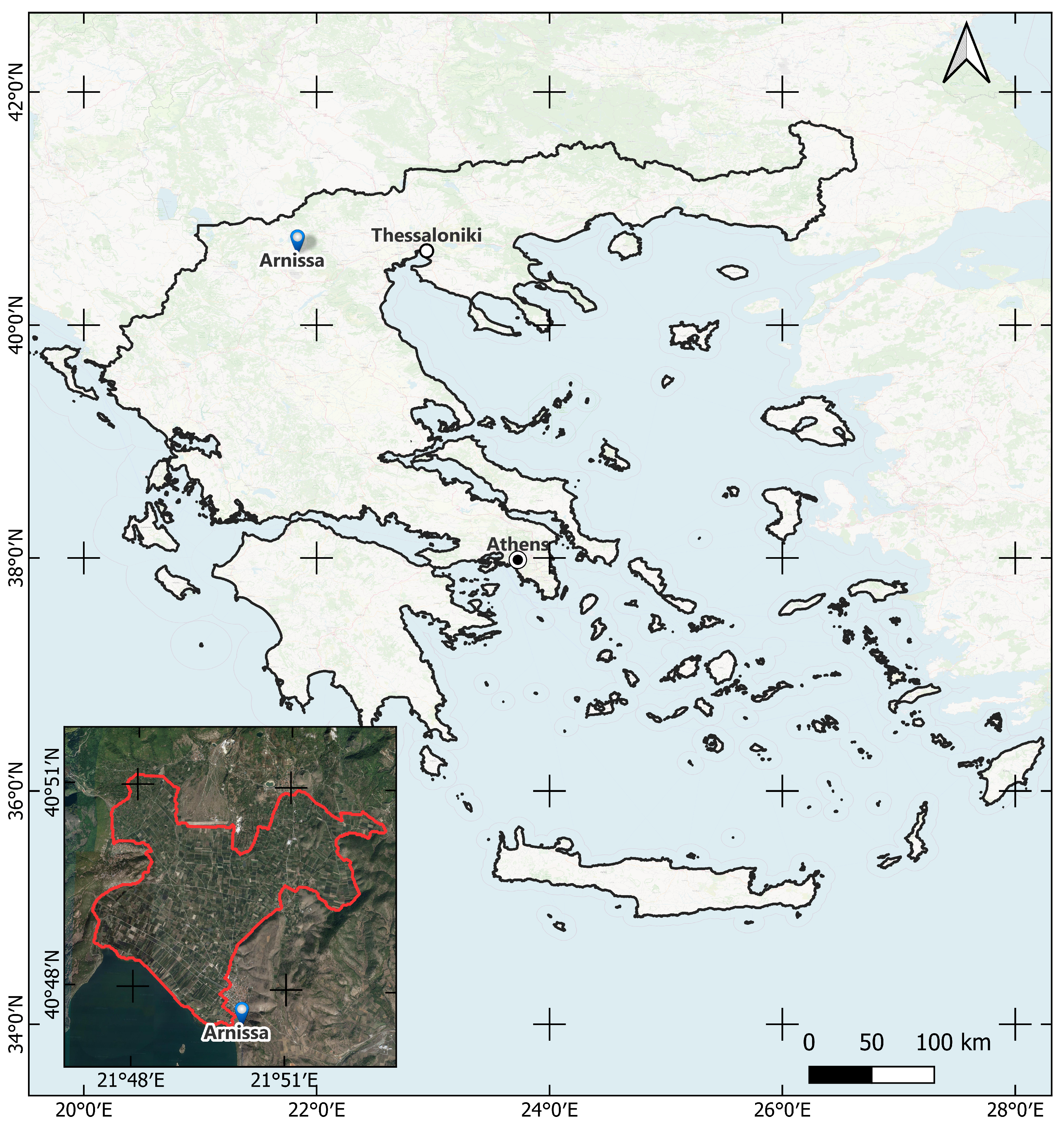
The study area, Figure 2 is located Northwest of the town of Arnissa, in the Pella regional unit, approximately 115 km West–Northwest of Thessaloniki, in northern Greece. This rural region is primarily recognized for its fruit plantations, predominantly consisting of stone fruits and pome fruits. Other minor plantations include tree nut plantations and vineyards. Hyperspectral data require preprocessing to address sensor artifacts, remove noise, correct atmospheric conditions, and enhance the overall data quality to facilitate accurate analysis.

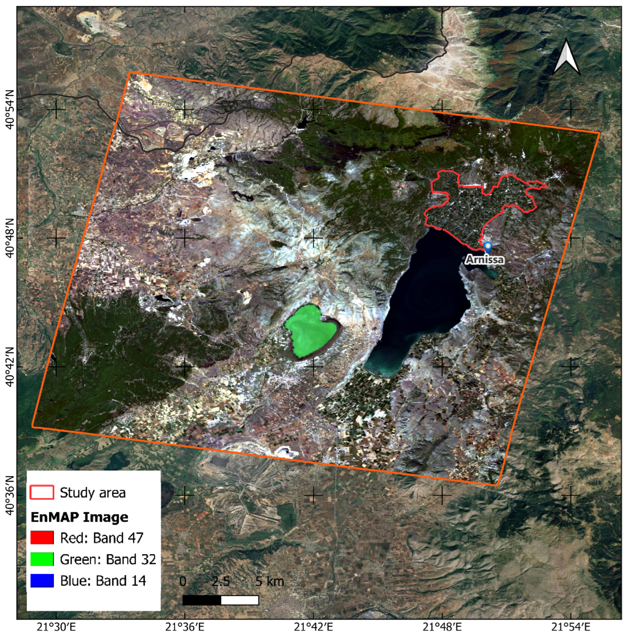
In this study, EnMAP hyperspectral imagery was utilized. The Environmental Mapping and Analysis Program (EnMAP) represents a German satellite initiative focused on hyperspectral observation aimed at systematically assessing and characterizing the Earth’s environmental conditions on a global scale. EnMAP effectively quantifies geochemical, biochemical, and biophysical parameters, thereby providing essential insights into the status and dynamics of both terrestrial and aquatic ecosystems.

The EnMAP mission, launched in 2022, is equipped with a duo of spectrometers that capture electromagnetic radiation across the visible spectrum to the shortwave infrared range, encompassing 246 distinct bands. EnMAP possesses a spatial resolution of 30 m by 30 m and exhibits a temporal revisit interval of 27 days, with an off-nadir revisit capability of four days. The spectral sampling interval varies between 6.5 nm (VNIR) and 12 nm (SWIR), allowing for detailed spectral resolution [42]. The EnMAP data are freely accessible to the scientific community via the official Data Access Portal (https://planning.enmap.org/ (20 August 2023)), subject to a mandatory user registration process. The acquisition date of the EnMAP image was 7 October 2022, coinciding with the collection of crop mapping ground truth data from the official Greek Payment Authority Common Agricultural Policy database in the same year.

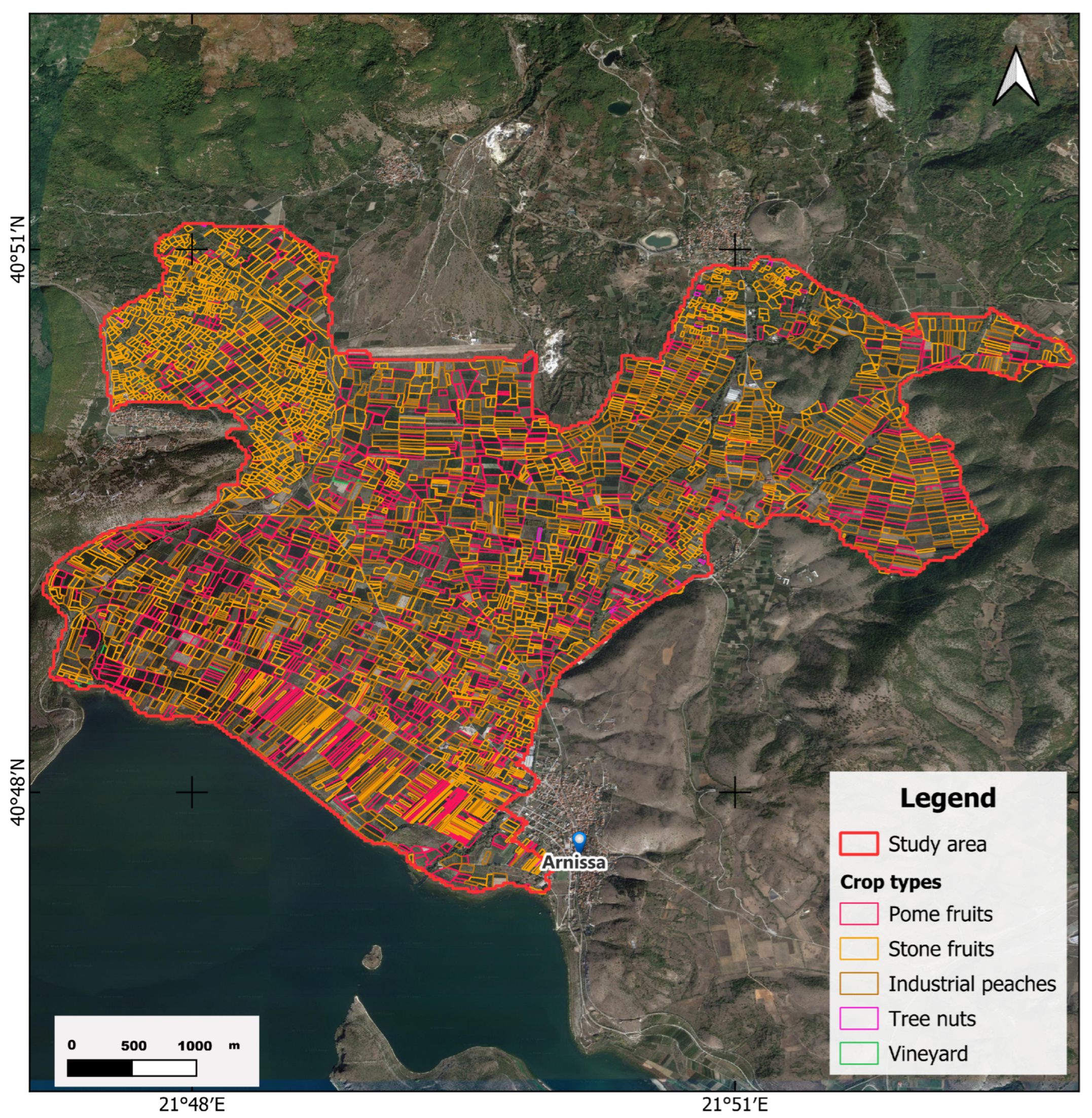
The ground truth data, Figure 3, were received from the Greek Payment Authority of Common Agricultural Policy. The data were received in shapefile format for the study area. In the study area, there are in total 4103 cultivated parcels: 1314 pome fruits, 2749 stone fruits, of which 867 are registered as industrial peach, 33 tree nuts, and 7 vineyards.

Bad/Overlapping Band Removal: Due to the existence of two different spectrometers (VNIR and SWIR), spectral overlap occurs between 900 nm and 1000 nm (from 902.2 nm to 993.0 nm). To avoid possible mismatches or co-registration errors between the sensors, overlapping VNIR bands were excluded from the analysis. Additionally, spectrally degraded or unreliable bands—such as those affected by sensor artifacts, strong water vapor absorption, or other anomalies—were excluded by referencing the image’s XML metadata file, where bad bands are flagged with a value of zero (0). After this procedure, 208 spectral bands remained for initial consideration.

Noise Removal and Minimum Noise Fraction (MNF) Transformation: Hyperspectral data inherently contain noise from various sources, including sensor characteristics, atmospheric interference, and environmental conditions. To address this, the Minimum Noise Fraction (MNF) transformation was applied [42]. MNF reduces noise and dimensionality by decorrelating and segregating noise from meaningful signals. It projects data into a new coordinate system ordered by their signal-to-noise ratios. The initial MNF components with high eigenvalues were retained as they encapsulate significant spectral information while suppressing noise and redundancy. Specifically, seven MNF bands from the VNIR range and two MNF bands from the SWIR range were retained. Subsequently, the inverse MNF transformation was applied separately to VNIR and SWIR data due to differing signal-to-noise ratios, projecting them back into their original spectral dimensions while minimizing noise.

2.2. Preprocessing and Band Orientation

Pre-processing of the EnMAP imagery was performed using ENVI software (ENVI 6.0). The EnMAP image was initially provided as Level-2A atmospherically corrected surface reflectance data. Preprocessing included the removal of spectrally degraded or unreliable bands based on the XML metadata flags and addressing sensor overlaps between the VNIR and SWIR spectrometers. This stage resulted in 208 bands, of which 196 bands were ultimately retained for further analysis following noise reduction via MNF transformation and visual assessment.

The judicious reduction in hyperspectral dimensionality plays a decisive role in remote-sensing analytics. When dozens or hundreds of highly correlated bands are left unfiltered, the resulting parameter space inflates computational demands, aggravates multicollinearity, and triggers the Hughes effect, whereby classifier performance deteriorates as dimensionality outpaces the availability of labelled samples [12]. By isolating—or projecting onto—a limited set of spectrally and statistically salient features, one can suppress sensor noise, discard atmospheric redundancy, and stabilize covariance estimates, all while shortening training times for machine-learning models. Equally important, a compact spectral signature clarifies the physical interpretation of class separability, revealing the wavelengths that truly govern biogeochemical or land-cover distinctions.

From a practical standpoint, early-stage dimensionality reduction decreases storage and transmission loads—an asset in large-area or near-real-time monitoring pipelines—while guarding against overfitting when ground truth is scarce. For these reasons, a carefully designed dimensionality-reduction step is not an optional convenience but rather a prerequisite for extracting robust, reproducible, and scientifically meaningful information from hyperspectral data. Following a visual assessment of the MNF-inverted dataset, 196 out of the original 208 EnMAP spectral bands were retained for further analysis based on their information content and spectral quality. The outcome of this process is demonstrated in Figure 4. The selected bands, along with their corresponding central wavelengths, are listed in

Table 1. Overview of EnMAP hyperspectral bands and their corresponding wavelengths.

EnMAP	$\mathit{\lambda }$nm	MNF Inv.	EnMAP	$\mathit{\lambda }$nm	MNF Inv.	EnMAP	$\mathit{\lambda }$nm	MNF Inv.	EnMAP	$\mathit{\lambda }$nm	MNF Inv.	EnMAP	$\mathit{\lambda }$nm	MNF Inv.	EnMAP	$\mathit{\lambda }$nm	MNF Inv.
Band 1	418.13	1	Band 35	587.88	35	Band 79	895.37	69	Band 113	1247.31	103	Band 147	1759.83	137	Band 183	2249.66	171
Band 2	423.76	2	Band 36	593.48	36	Band 80	903.45	70	Band 114	1259.3	104	Band 149	1948.98	138	Band 184	2257.86	172
Band 3	429.19	3	Band 37	599.15	37	Band 81	911.55	71	Band 115	1271.29	105	Band 151	1967.95	139	Band 185	2266.04	173
Band 4	434.42	4	Band 38	604.89	38	Band 82	919.66	72	Band 116	1283.29	106	Band 152	1977.37	140	Band 186	2274.18	174
Band 5	439.5	5	Band 39	610.71	39	Band 83	927.79	73	Band 117	1295.28	107	Band 153	1986.74	141	Band 187	2282.29	175
Band 6	444.45	6	Band 40	616.61	40	Band 84	935.92	74	Band 118	1307.27	108	Band 154	1996.07	142	Band 188	2290.37	176
Band 7	449.3	7	Band 41	622.61	41	Band 85	944.05	75	Band 119	1319.25	109	Band 155	2005.36	143	Band 189	2298.42	177
Band 8	454.06	8	Band 42	628.67	42	Band 86	952.19	76	Band 120	1461.46	110	Band 156	2014.61	144	Band 190	2306.44	178
Band 9	458.79	9	Band 53	699.43	43	Band 87	960.33	77	Band 121	1473.1	111	Band 157	2023.82	145	Band 191	2314.42	179
Band 10	463.49	10	Band 54	706.26	44	Band 88	968.47	78	Band 122	1484.69	112	Band 158	2032.99	146	Band 192	2322.37	180
Band 11	468.17	11	Band 55	713.17	45	Band 89	976.62	79	Band 123	1496.24	113	Band 159	2042.11	147	Band 193	2330.29	181
Band 12	472.84	12	Band 56	720.14	46	Band 90	984.77	80	Band 124	1507.75	114	Band 160	2051.19	148	Band 194	2338.19	182
Band 13	477.51	13	Band 57	727.18	47	Band 91	992.92	81	Band 125	1519.22	115	Band 161	2060.24	149	Band 195	2346.05	183
Band 14	482.17	14	Band 58	734.29	48	Band 92	1004.21	82	Band 126	1530.64	116	Band 162	2069.24	150	Band 196	2353.88	184
Band 15	486.85	15	Band 59	741.46	49	Band 93	1015.05	83	Band 127	1542.02	117	Band 163	2078.21	151	Band 197	2361.68	185
Band 16	491.54	16	Band 60	748.68	50	Band 94	1026	84	Band 128	1553.36	118	Band 164	2087.13	152	Band 198	2369.45	186
Band 17	496.25	17	Band 61	755.97	51	Band 95	1037.05	85	Band 129	1564.65	119	Band 165	2096.01	153	Band 199	2377.19	187
Band 18	501	18	Band 62	763.32	52	Band 96	1048.19	86	Band 130	1575.9	120	Band 166	2104.86	154	Band 200	2384.9	188
Band 19	505.77	19	Band 63	770.72	53	Band 97	1059.42	87	Band 131	1587.1	121	Band 167	2113.67	155	Band 201	2392.58	189
Band 20	510.58	20	Band 64	778.18	54	Band 98	1070.74	88	Band 132	1598.26	122	Band 168	2122.44	156	Band 202	2400.23	190
Band 21	515.42	21	Band 65	785.69	55	Band 99	1082.14	89	Band 133	1609.36	123	Band 169	2131.17	157	Band 203	2407.85	191
Band 22	520.3	22	Band 66	793.25	56	Band 100	1093.62	90	Band 134	1620.43	124	Band 170	2139.87	158	Band 204	2415.45	192
Band 23	525.21	23	Band 67	800.85	57	Band 101	1105.17	91	Band 135	1631.44	125	Band 171	2148.52	159	Band 205	2423.01	193
Band 24	530.17	24	Band 68	808.51	58	Band 102	1116.79	92	Band 136	1642.41	126	Band 172	2157.15	160	Band 206	2430.55	194
Band 25	535.16	25	Band 69	816.21	59	Band 103	1128.47	93	Band 137	1653.33	127	Band 173	2165.73	161	Band 207	2438.05	195
Band 26	540.2	26	Band 70	823.96	60	Band 104	1140.2	94	Band 138	1664.2	128	Band 174	2174.28	162	Band 208	2445.53	196
Band 27	545.29	27	Band 71	831.74	61	Band 105	1151.98	95	Band 139	1675.03	129	Band 175	2182.79	163
Band 28	550.42	28	Band 72	839.57	62	Band 106	1163.81	96	Band 140	1685.8	130	Band 176	2191.27	164
Band 29	555.6	29	Band 73	847.44	63	Band 107	1175.67	97	Band 141	1696.53	131	Band 177	2199.71	165
Band 30	560.84	30	Band 74	855.35	64	Band 108	1187.56	98	Band 142	1707.2	132	Band 178	2208.12	166
Band 31	566.13	31	Band 75	863.29	65	Band 109	1199.48	99	Band 143	1717.83	133	Band 179	2216.5	167
Band 32	571.48	32	Band 76	871.27	66	Band 110	1211.42	100	Band 144	1728.4	134	Band 180	2224.84	168
Band 33	576.89	33	Band 77	879.28	67	Band 111	1223.37	101	Band 145	1738.93	135	Band 181	2233.14	169
Band 34	582.35	34	Band 78	887.32	68	Band 112	1235.34	102	Band 146	1749.4	136	Band 182	2241.42	170

.

2.3. Decision Making

Semantic segmentation of Earth-observation imagery demands models that can preserve fine spatial detail while reasoning over broader context. Architectures derived from the U-Net lineage fulfill these requirements by combining a contracting encoder path, which gathers multi-scale semantic features, with a symmetric expanding decoder that restores full resolution through explicit skip-connections. The present work evaluates three successive members of this family—standard U-Net, U-Net++, and an atrous-enabled U-Net variant—in order to quantify the incremental benefits of deeper fusion and multi-scale context aggregation.

The study adopted the U-Net family of convolutional neural networks —namely the original U-Net, U-Net++, and an atrous (dilated-convolution) U-Net—because this encoder–decoder paradigm offers a judicious balance of architectural parsimony, data-efficiency, and spatial fidelity that is well suited to hyperspectral scene analysis. A symmetric contracting–expanding path with skip connections preserves fine-grained localization while simultaneously aggregating high-level semantic context, thereby enabling precise pixel-wise delineation even when training data are scarce—a frequent constraint in remote-sensing campaigns.

The nested dense skip connections of U-Net++ refine feature fusion across multiple semantic scales, mitigating the semantic gap between encoder and decoder and often accelerating convergence. Conversely, the introduction of atrous convolutions enlarges the receptive field without inflating the parameter count, allowing the atrous variant to capture long-range contextual cues that are essential for resolving spectrally similar but spatially dispersed classes. Collectively, these three complementary configurations provide a systematic framework for interrogating the trade-offs between model complexity, receptive-field size, and segmentation accuracy, while retaining a common backbone whose proven robustness in biomedical imaging has translated effectively to hyperspectral land-cover mapping.

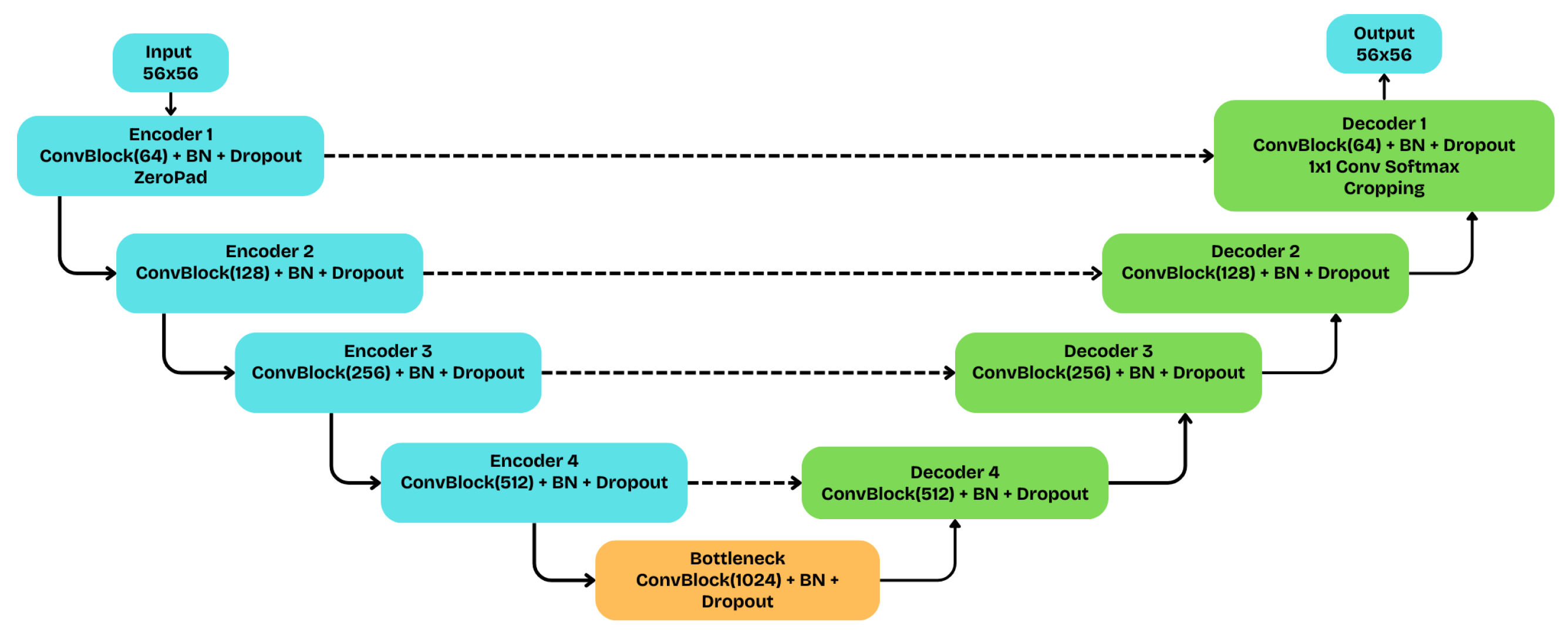
The implemented baseline U-Net, whose fundamental structure is schematically depicted in Figure 5, adopts a symmetric five-level encoder (blue) - decoder (green) topology. In the contracting path (encoder), each level consists of a convolutional block with two sequential $3\times 3$ convolutions, each followed by Batch Normalization and a ReLU activation. Spatial downsampling is achieved through a $2\times 2$ max-pooling operation, while the number of filters doubles at each step, starting from 64 and reaching 1024 at the bottleneck. For regularization and to prevent overfitting, a Dropout layer with a rate of 0.1 (10%) is applied at the end of each convolutional block.

In the symmetric expansive path (decoder), spatial resolution is restored via a $2\times 2$ upsampling (UpSampling2D) process. At each level, the upsampled feature map is concatenated with the corresponding map from the encoder via skip connections, thereby reintroducing high-resolution spatial information. To handle input image patches with dimensions not perfectly divisible by 32 ($2^5$), the model applies a strategy of zero-padding at the input and corresponding cropping at the output. The network terminates with a $1\times 1$ convolution and a softmax activation, which produces the final class probabilities for each pixel. This architecture balances depth with parameter economy, making it suitable for the semantic segmentation of hyperspectral data.

The implemented U-Net++ architecture, whose fundamental structure is schematically depicted in Figure 6, extends the classic U-Net by introducing a set of nested and densely connected skip pathways. This approach is designed to bridge the semantic gap between encoder and decoder features, improving segmentation quality.

This specific implementation is a shallower variant with a depth of three levels.The encoder (blue) processes the input through three stages, with filter counts of 64, 128, and 256, respectively. Each convolutional block consists of two $3\times 3$ convolutions with ReLU activation. Unlike other configurations, this architecture omits Batch Normalization but incorporates Dropout with a rate of 0.1 at the end of each block for regularization.

The nested skip pathways allow for the gradual accumulation of features. The final segmentation map is generated from node $x_{0,2}$, which combines features from three different sources: the initial encoder feature map ($c_1$), the first-level skip node ($x_{0,1}$), and the upsampled deeper node ($x_{1,1}$). This dense connectivity enables the network to produce sharp object boundaries. The final prediction is delivered by a $1\times 1$ convolutional layer with a softmax activation, creating the probability cube for each pixel.

The architecture of the Atrous U-Net network, the fundamental structure of which is schematically depicted in Figure 7, is a Squeeze-and-Excitation (SE) dilated U-Net, designed to enlarge the receptive field without degrading spatial resolution. Along the encoder path (blue), the dilation rate doubles at each of the five stages—$1\to 2\to 4\to 8\to 16$—while the number of filters increases from 64 to 1024. Each convolutional block now incorporates not only two dilated convolutions but also Batch Normalization, a Squeeze-and-Excitation (SE) module with a reduction ratio of 16, and Dropout regularization with a rate of 0.1. The SE mechanism allows the model to dynamically recalibrate channel-wise feature responses, thereby emphasizing the most informative ones. To ensure dimensional compatibility during the successive downsampling operations of the encoder, a strategy of zero-padding at the input and corresponding cropping at the output is adopted.

In summary, the three U-Net variants examined here offer complementary routes to reconciling spectral richness with spatial precision.

The baseline U-Net supplies a lean, well-tested backbone whose encoder–decoder symmetry and direct skip connections already yield reliable pixel-level delineation. Building on that foundation, U-Net++ densifies the skip topology, narrowing the semantic gap between encoding and decoding stages and thereby sharpening object boundaries without a prohibitive rise in parameters. Finally, the atrous U-Net enlarges the receptive field through systematic dilation, endowing the network with long-range contextual awareness that is especially beneficial when class separability hinges on broader scene structure. All these architectures map a spectrum of design trade-offs—depth versus width, locality versus context—providing a robust experimental framework from which the most task-appropriate configuration, or an ensemble thereof, can be selected for operational hyperspectral segmentation.

3. Experimental Setup

This section outlines the experimental design adopted to evaluate the impact of different dimensionality-reduction strategies on hyperspectral crop classification with U-Net-based architectures. Our analysis was conducted using the EnMAP hyperspectral scene described in Section 2, combined with parcel-level ground truth data for multiple perennial crop classes. To ensure rigorous evaluation, we designed a parcel-based spatial holdout with buffer enforcement, thereby preventing information leakage due to spatial autocorrelation.

We investigated four complementary band selection approaches, chosen to represent statistical, model-driven, and unsupervised paradigms. Specifically, (i) Linear Discriminant Analysis (LDA) was employed as a supervised projection method that maximizes class separability; (ii) SHAP-based feature attribution was applied on an XGBoost baseline to identify the most informative bands, yielding compact yet interpretable subsets; (iii) Agglomerative Clustering Selection (ACS) was used as an unsupervised strategy to group spectrally redundant bands and retain a representative subset (196 to 60 bands) and (iv) Orthogonal Matching Pursuit (OMP) was implemented as a sparse approximation technique to recover the most discriminative features. These reduced feature sets were subsequently used as inputs to the three deep architectures under study: U-Net, U-Net++, and Atrous U-Net.

The combination of diverse band selection methods and deep segmentation models provides a systematic framework to evaluate how different spectral representations interact with network design, thereby allowing us to disentangle architectural effects from data-related factors.

3.1. Spectral Band Selection via Statistical and Model-Driven Methods

Dimensionality reduction plays a critical role in hyperspectral image analysis by addressing challenges such as spectral redundancy, sensor noise, and the curse of dimensionality. To comprehensively explore this design space, we adopted a diverse set of supervised and unsupervised strategies for band selection. Specifically, two supervised techniques were implemented: a statistical method based on Linear Discriminant Analysis (LDA) with sequential feature selection, and a model-driven approach using SHAP (SHapley Additive exPlanations) values derived from gradient-boosted decision trees. To complement these, two unsupervised schemes were further introduced: a distribution-based clustering method leveraging Jensen–Shannon divergences between band histograms, and a reconstruction-driven greedy selection procedure inspired by column subset selection. Together, these approaches provide a multifaceted view of the problem, balancing statistical optimality, model interpretability, and data-driven compactness without reliance on class labels.

The first approach combines LDA with a forward Sequential Feature Selection (SFS) wrapper. After removing unknown class pixels from the Vegoritida hyperspectral cube, a class-stratified bootstrap sample of 5000 valid pixels was drawn to mitigate imbalance. The SFS algorithm iteratively added bands that maximized five-fold cross-validated LDA accuracy. Although up to 15 bands were evaluated, an inspection of the LDA loadings revealed that six spectral channels—TIF indices, as shown in

Table 2. LDA image channels reduction implementation outcomes.

Bands Retained by SFS–LDA
30	32	47	52	60	74

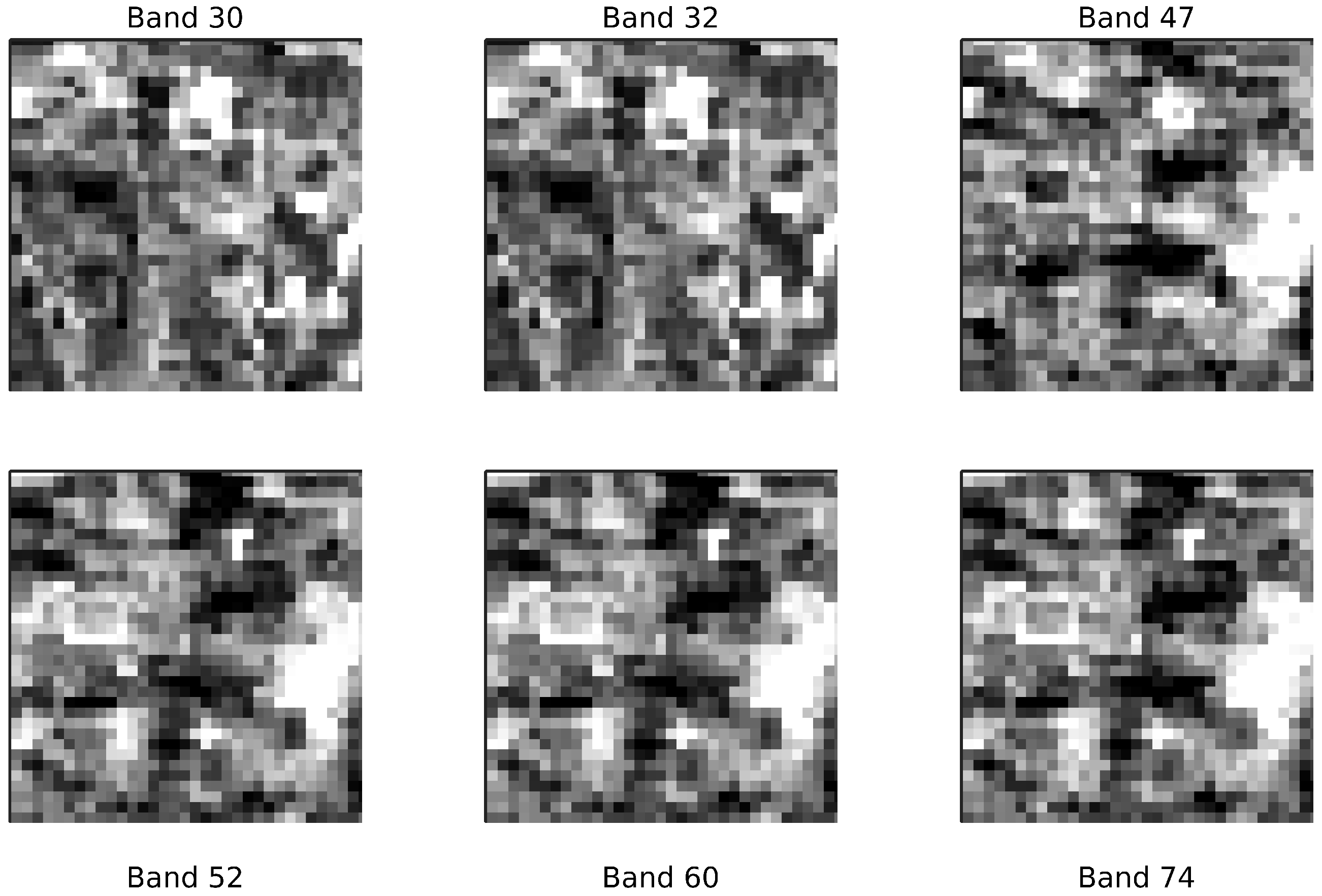
, captured the entire discriminative variance (explained-variance ratio = 1.00) and accounted for approximately 92% of the aggregate importance. Figure 8 provides an indicative visualization for all of these bands, over a randomly selected image patch. These bands were selected to construct a compact six-band GeoTIFF, facilitating both efficient storage and faster model training. All band rankings and component variances were exported to CSV for reproducibility and future analysis.

The second dimensionality-reduction method follows a model-centered strategy based on gradient-boosted decision trees (XGBoost). After removing unknown class values, a stratified 70/30 partition split under a fixed random seed was used. The class imbalance was mitigated via inverse-frequency sample weights. A conservative, lightweight configuration of 100 boosting rounds, using multiclass log-loss optimization, was adopted, including a fixed seed, to minimize overfitting and avoid injecting tuning bias into subsequent attributions. All other parameters maintained the scikit-learn library’s default values.

To prevent information leakage, SHAP attributions (i.e., TreeExplainer) were computed only on the training split. A transparent, reproducible selection rule defined the reduced subset: a band was retained if it appeared in the per-class top-5 for at least two crop classes or if its global mean $\left|\mathrm{SHAP}\right|$ exceeded the 75th percentile; the final subset size was fixed at 19 bands. Using the same stratified split, balanced weights, and seed, the 19-band model achieved OA = 0.747 and macro-F1 = 0.740 on the held-out test set, versus OA = 0.762 and macro-F1 = 0.756 with all 196 bands ($\Delta$OA = $-1.52$ pp; $\Delta$macro-F1 = $-1.67$ pp; 95% bootstrap CI for $\Delta$OA: $-1.83$ to $-1.25$ pp). This represents a modest performance reduction given the 90.3% dimensionality decrease ($196\to 19$), a trade-off that substantially improves parsimony and interpretability while preserving nearly all predictive signal.

The TIF band indices that were retained by the SHAP analysis are presented in

Table 3. SHAP image channels reduction implementation outcomes.

Bands Retained by SHAP Analysis
1	2	3	24	25
27	28	42	44	45
46	47	48	49	52
54	74	77	82

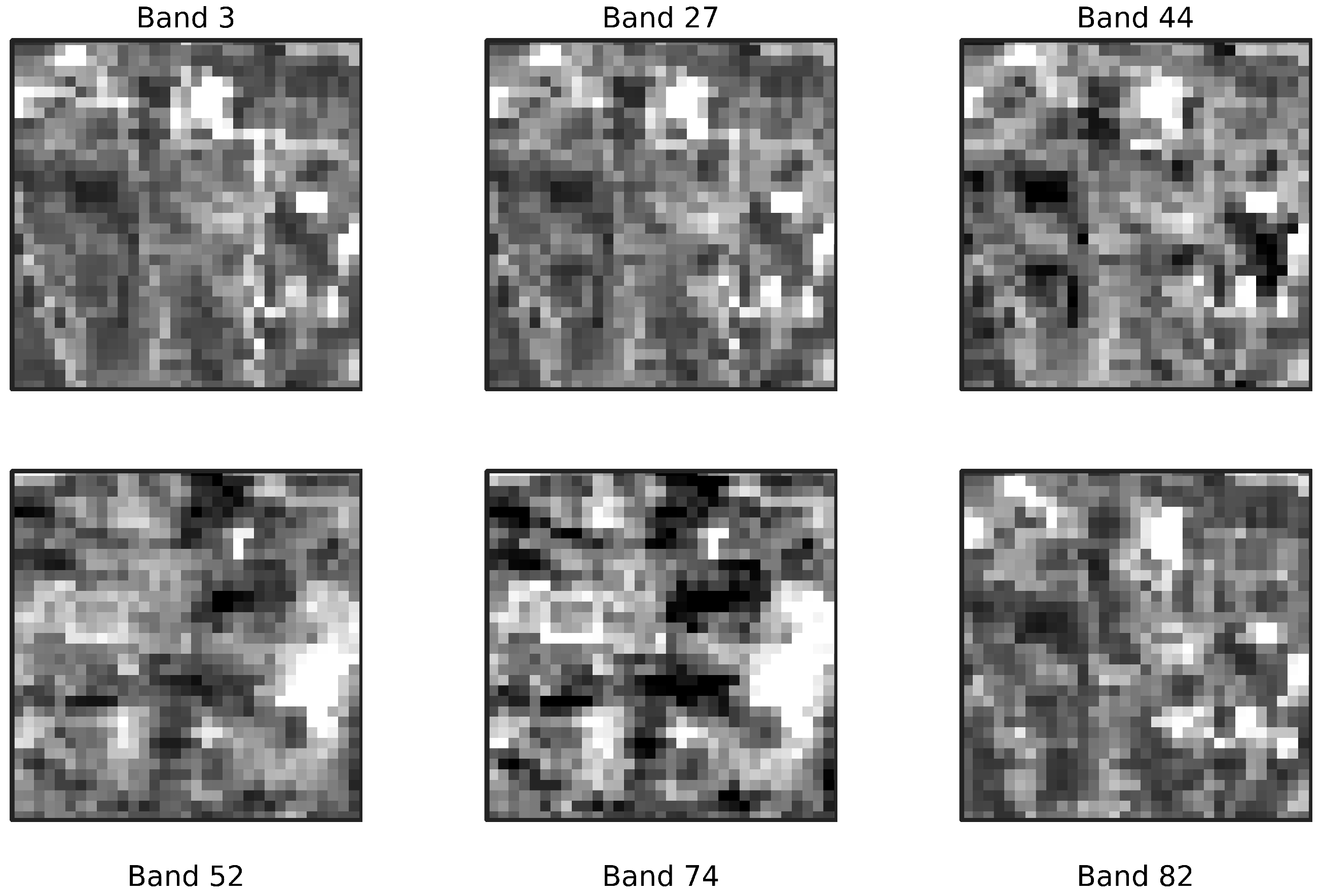
. Figure 9 provides an indicative visualization for 6 out of the 19 selected bands, over a randomly selected image patch.

An unsupervised Histogram-based clustering (Agglomerative) strategy was also introduced to identify representative spectral channels based on the similarity of their value distributions. Each band, with pixel values inherently in the surface reflectance range of $[0, 1]$, was then converted into a probability histogram (30 bins with common edges). The pairwise divergence between histograms was quantified using the Jensen–Shannon distance, a symmetric and bounded metric well-suited for spectral distribution comparison. The resulting distance matrix was clustered via Agglomerative Clustering with average linkage, targeting a reduced subset corresponding to 30% of the original dimensionality ($196\to 59$ bands). Within each cluster, the medoid band—i.e., the one with the minimum cumulative divergence to its peers—was retained as representative. The selected bands span both contiguous and non-contiguous regions of the spectrum, suggesting that distributional diversity is effectively captured. The full set of indices is reported in

Table 4. Agglomerative histogram-clustering image channels reduction implementation outcomes.

Bands Retained by Agglomerative Histogram-Clustering (59)
0	1	4	7	12	14
20	21	22	23	24	25
27	31	32	36	40	42
43	44	45	46	47	48
53	57	61	67	70	71
73	75	78	82	85	91
92	93	94	97	102	108
110	113	114	115	116	119
125	130	133	137	138	141
146	165	182	186	195

.

A second unsupervised approach, based on Greedy reconstruction-driven selection, was designed to select bands that best preserve the global variance structure of the hyperspectral cube. Inspired by column subset selection methods, we adopted a greedy procedure akin to Orthogonal Matching Pursuit (OMP): at each step, the band that minimized the residual reconstruction error of the covariance matrix was added to the subset. This criterion ensures that the chosen bands collectively span the spectral feature space with minimal redundancy. Fixing the target subset size to 30% of the spectrum yielded 59 bands, covering diverse regions while maintaining linear representational capacity. Compared with clustering-based methods, this reconstruction-driven strategy emphasizes global covariance preservation rather than distributional dissimilarity. The selected band indices are given in

Table 5. OMP image channels reduction implementation outcomes.

Bands Retained by Reconstruction-Driven Selection (59)
0	3	5	7	17	19
21	22	27	42	46	52
56	57	59	60	61	62
63	64	66	68	69	71
72	73	74	75	76	77
78	80	81	86	88	98
105	109	110	111	117	129
136	137	138	140	141	143
145	148	156	166	175	177
187	188	189	191	195

.

In summary, the four dimensionality-reduction strategies explored in this, i.e., SFS–LDA, SHAP, histogram-based clustering, and reconstruction-driven selection, offer complementary perspectives on hyperspectral band selection. While the supervised methods emphasize discriminative power and predictive accuracy, the unsupervised schemes prioritize redundancy reduction and preservation of intrinsic spectral structure. This methodological diversity ensures that both class-separability and data-intrinsic criteria are represented, yielding compact subsets that are efficient, interpretable, and well-suited as inputs for the comparative evaluation of U-Net architectures in subsequent experiments.

3.2. Dataset Preparation

The dataset preparation begins with the spatial alignment of the hyperspectral cube and the ground-truth data to ensure geometric consistency. Next, a sliding window of a fixed size of $56\times 56$ pixels is applied with a stride of two pixels to generate a dense set of overlapping patches. Each patch is subjected to a quality control step: if more than 40% of its pixels correspond to unknown class values, the patch is discarded.

Importantly, the use of spatial patches, rather than single-pixel spectral vectors, captures essential contextual information that would otherwise be lost [43,44]. While per-pixel approaches leverage the spectral signature of each point, they ignore the spatial structure of the surrounding area, which often contains crucial clues for differentiating between spectrally similar crop types. By incorporating both spatial and spectral information, the patch-based method supports more robust feature learning, especially in the presence of intra-class variability or noise.

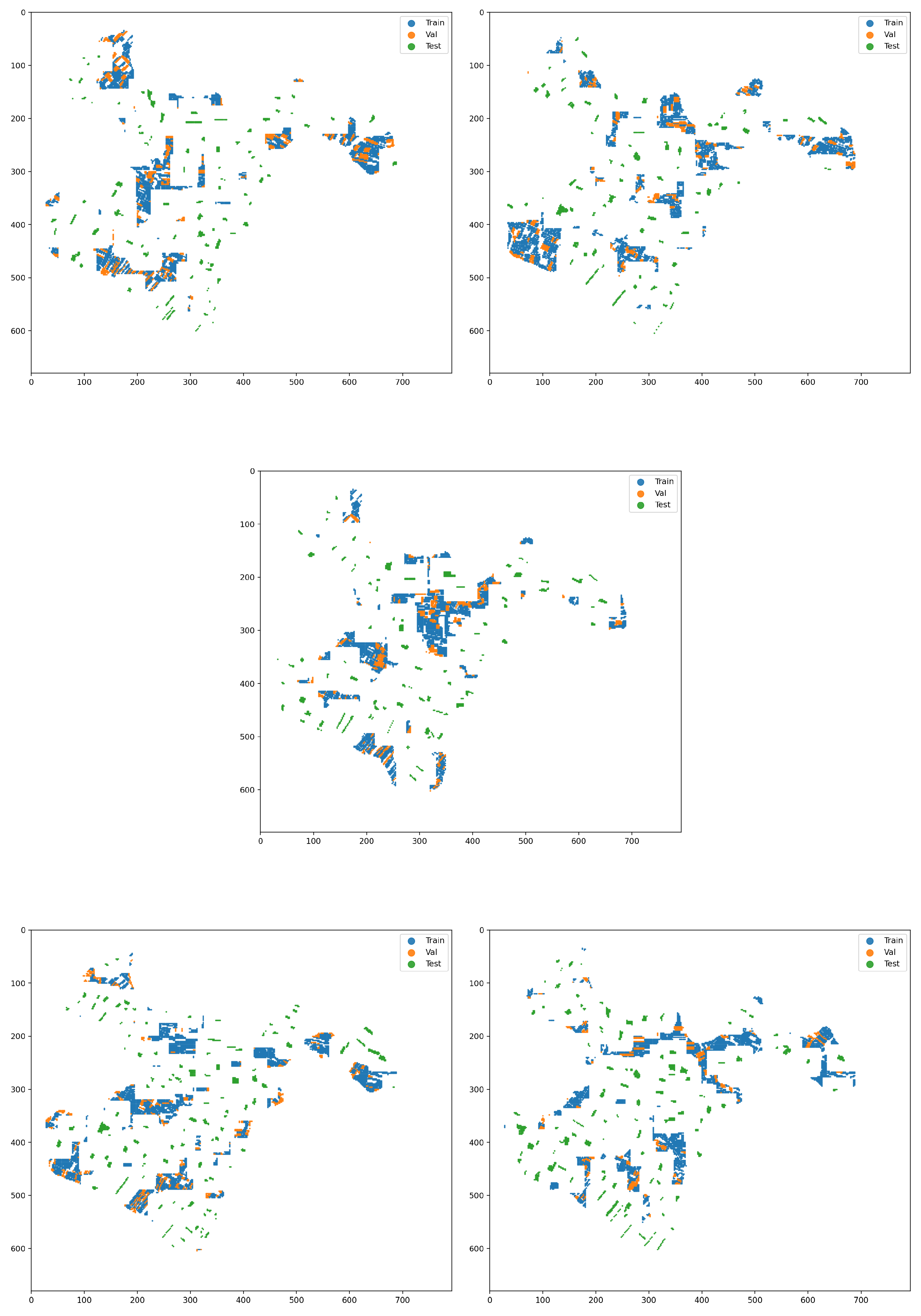
To address the critical issue of spatial autocorrelation and to avoid overly optimistic performance estimates, a strict data splitting strategy, known as a spatial holdout, was adopted (see Figure 10). Instead of a random sampling of patches, which would lead to information leakage between the training and evaluation sets, the new procedure leverages the boundaries of agricultural parcels provided in a shapefile. Specifically, all patches originating from the same parcel are grouped together, and the division into training (70%), validation (15%), and test (15%) sets is performed at the parcel level. This guarantees that entire parcels are exclusively assigned to one of the three sets, ensuring that the model is trained and evaluated on geographically distinct and independent regions.

To achieve absolute spatial isolation and eliminate any possibility of contact, the methodology dynamically defines a buffer zone around the parcels of the test set. The width of this zone is automatically set to be equal to the patch radius plus one additional pixel (radius + 1). The rejection of patches is based on the position of their central pixel (centroid): if the center of a training or validation patch falls within this buffer zone, the entire patch is discarded. Because the buffer is larger than the distance from the patch’s center to its edge, this strategy guarantees that there will always be a minimum distance of one pixel between any training/validation patch and the test area. Consequently, the datasets not only do not overlap, but also do not even touch.

Finally, normalization statistics (mean and standard deviation) are calculated exclusively from the training data to prevent any information leakage. The normalized patches and their corresponding masks are stored in HDF5 files for optimized I/O speed during training. To ensure statistical reliability and to rule out the possibility of chance results, the entire experimental procedure, from the spatial split to the final training, is repeated five times using five different random seeds. Each seed produces a different but equally valid spatial split of the data. Critically, this set of five seeds remained fixed across all evaluated architectures, providing a consistent and unbiased basis for comparing their performance.

3.3. Model Training and Optimization

To investigate the performance of different architectures and select the appropriate model for the data, a structured random search strategy was adopted to ensure the reproducibility and interpretability of the findings. This approach allowed for an effective exploration of a broad, discrete hyperparameter space in a controlled and systematic manner.

All models were trained, validated, and tested on a dataset consisting of image patches, which was split into 500 training, 500 validation, and 500 test samples.

Initially, for each of the three model families (U-Net, U-Net++, Atrous U-Net), a search space was defined that included all possible combinations of critical hyperparameters (

Table 6. Hyperparameter Search Space per Model Family.

Hyperparameter	U-Net	U-Net++	Atrous U-Net
Network Depth	{3, 4, 5}	{3, 4, 5}	{3, 4, 5}
Dropout Rate	{0.1, 0.2, 0.3}	{0.1, 0.2, 0.3}	{0.1, 0.2, 0.3}
Batch Normalization	{True, False}	{True, False}	{True, False}
SE Reduction Ratio	-	-	{8, 16, 32}

).

From this complete space, 10 unique architectures were randomly sampled for each family, leading to a total of 30 experiments. The sampling process was initialized with a fixed seed to guarantee the full reproducibility of the results. Regarding the remaining parameters, the learning rate was held constant at $1\times {10}^{-3}$ for all trials, a widely accepted value for the Adam optimizer that ensures a fair comparison between architectures.

The final selection of the best architecture from each family was based on a clear criterion: the highest macro F1-score on the validation set. This metric was chosen as it provides a balanced assessment of performance in multi-class classification problems. All the models that were tested (

Table 7. Evaluated architectures during the random search grid process.

Family	Depth	Encoder Filters	Decoder Filters	Dropout	Batch Norm	Se Reduction	Dilations Encoder	Val F1 Macro
U-Net	5	[64, 128, 256, 512, 1024]	[512, 256, 128, 64]	0.3	True	-	-	0.2260
U-Net	5	[64, 128, 256, 512, 1024]	[512, 256, 128, 64]	0.2	False	-	-	0.1348
U-Net	5	[64, 128, 256, 512, 1024]	[512, 256, 128, 64]	0.2	True	-	-	0.5946
U-Net	4	[64, 128, 256, 512]	[256, 128, 64]	0.3	False	-	-	0.5886
U-Net	4	[64, 128, 256, 512]	[256, 128, 64]	0.1	False	-	-	0.5994
U-Net	4	[64, 128, 256, 512]	[256, 128, 64]	0.1	True	-	-	0.5981
U-Net	4	[64, 128, 256, 512]	[256, 128, 64]	0.2	True	-	-	0.5803
U-Net	5	[64, 128, 256, 512, 1024]	[512, 256, 128, 64]	0.1	True	-	-	0.6082
U-Net	3	[64, 128, 256]	[128, 64]	0.3	False	-	-	0.5814
U-Net	3	[64, 128, 256]	[128, 64]	0.3	True	-	-	0.5526
U-Net++	4	[64, 128, 256, 512]	[64, 128, 256]	0.1	True	-	-	0.5965
U-Net++	5	[64, 128, 256, 512, 1024]	[64, 128, 256, 512]	0.3	False	-	-	0.5583
U-Net++	3	[64, 128, 256]	[64, 128]	0.1	False	-	-	0.6038
U-Net++	3	[64, 128, 256]	[64, 128]	0.3	True	-	-	0.2348
U-Net++	5	[64, 128, 256, 512, 1024]	[64, 128, 256, 512]	0.3	True	-	-	0.2682
U-Net++	4	[64, 128, 256, 512]	[64, 128, 256]	0.3	False	-	-	0.5837
U-Net++	4	[64, 128, 256, 512]	[64, 128, 256]	0.1	False	-	-	0.5857
U-Net++	3	[64, 128, 256]	[64, 128]	0.2	False	-	-	0.5935
U-Net++	5	[64, 128, 256, 512, 1024]	[64, 128, 256, 512]	0.1	True	-	-	0.5948
U-Net++	3	[64, 128, 256]	[64, 128]	0.3	False	-	-	0.5961
U-Net Atrus	5	[64, 128, 256, 512, 1024]	[512, 256, 128, 64]	0.1	False	32	[1, 2, 4, 8, 16]	0.5944
U-Net Atrus	3	[64, 128, 256]	[128, 64]	0.3	True	32	[1, 2, 4]	0.5717
U-Net Atrus	4	[64, 128, 256, 512]	[256, 128, 64]	0.3	True	16	[1, 2, 4, 8]	0.5549
U-Net Atrus	3	[64, 128, 256]	[128, 64]	0.3	False	8	[1, 2, 4]	0.5807
U-Net Atrus	5	[64, 128, 256, 512, 1024]	[512, 256, 128, 64]	0.1	True	16	[1, 2, 4, 8, 16]	0.6066
U-Net Atrus	3	[64, 128, 256]	[128, 64]	0.2	False	8	[1, 2, 4]	0.5880
U-Net Atrus	4	[64, 128, 256, 512]	[256, 128, 64]	0.2	False	16	[1, 2, 4, 8]	0.5909
U-Net Atrus	5	[64, 128, 256, 512, 1024]	[512, 256, 128, 64]	0.2	True	16	[1, 2, 4, 8, 16]	0.5999
U-Net Atrus	5	[64, 128, 256, 512, 1024]	[512, 256, 128, 64]	0.1	True	8	[1, 2, 4, 8, 16]	0.6054
U-Net Atrus	4	[64, 128, 256, 512]	[256, 128, 64]	0.2	True	16	[1, 2, 4, 8]	0.5884

), as well as those that were selected (

Table 8. The best performing architectures selected by family.

Family	Depth	Dropout	Batch Norm	Validation F1 Macro
U-Net	5	0.1	True	0.6082
U-Net++	3	0.1	False	0.6038
Atr U-Net	5	0.1	True	0.6066

), are presented below.

The training procedure was kept consistent across all experiments to ensure a fair comparison between the architectures (see

Table 9. Details of the training protocol applied across all experiments.

Parameter	Value
Epochs	50
Early Stopping	Yes (patience = 10)
Model Checkpoint	Save best on val_loss
Experimental Runs	5 independent runs (different seeds)
Training Set Split	70%
Validation Set Split	15%
Test Set Split	15%
Data Generator	Custom Keras Sequence
Patch Size	56 × 56
Stride	2
Label Encoding	No (Sparse Labels for classes)
Input Normalization	Yes (Z-score: per-band $\mu ,\sigma$)

). Each model was trained for a maximum of 50 epochs, employing an Early Stopping mechanism. This mechanism terminated the training if the validation loss (val_loss) did not improve for 10 consecutive epochs (patience = 10), thus preventing overfitting. Concurrently, a model checkpoint was used to always save the model state that achieved the lowest validation loss. For feeding the models, the data were organized into image patches with dimensions of 56 × 56 pixels, which were extracted with a stride of 2.

3.4. Experimental Results

The experimental process involves three U-Net variations and five hyperspectral band selection approaches, resulting in fifteen distinct model configurations. Each model configuration was trained and evaluated using identical preprocessed input data, corresponding to its specific spectral dimensionality. A holdout approach of five sets was applied, as explained in Section 3.3. Input tensors varied spectrally from 196 (all channels) to 6 bands (SFS-LDA), depending on the dimensionality reduction strategy, Section 2.2. The output consistently comprised a single-channel segmentation mask, for pixel-level crop classification.

The experiments reveal multiple key findings. First, dimensionality reduction enhances efficiency without compromising accuracy: ACS reduces the spectral space by nearly 70% (196 to 60 bands) while sustaining or improving performance, and SHAP achieves an even more compact representation (down to 19 bands, over 90% reduction) with competitive accuracy when paired with Atrous U-Net.

Second, U-Net++ generally delivers the strongest results, regardless of the band selection approach, reaching a peak mean F1-score of 0.77 with ACS-selected bands. Third, class-level analysis shows that spectrally similar crops such as nut trees and industrial peach remain the most challenging, whereas vineyards and stone fruits are consistently well distinguished. These highlights set the stage for the detailed results that follow.

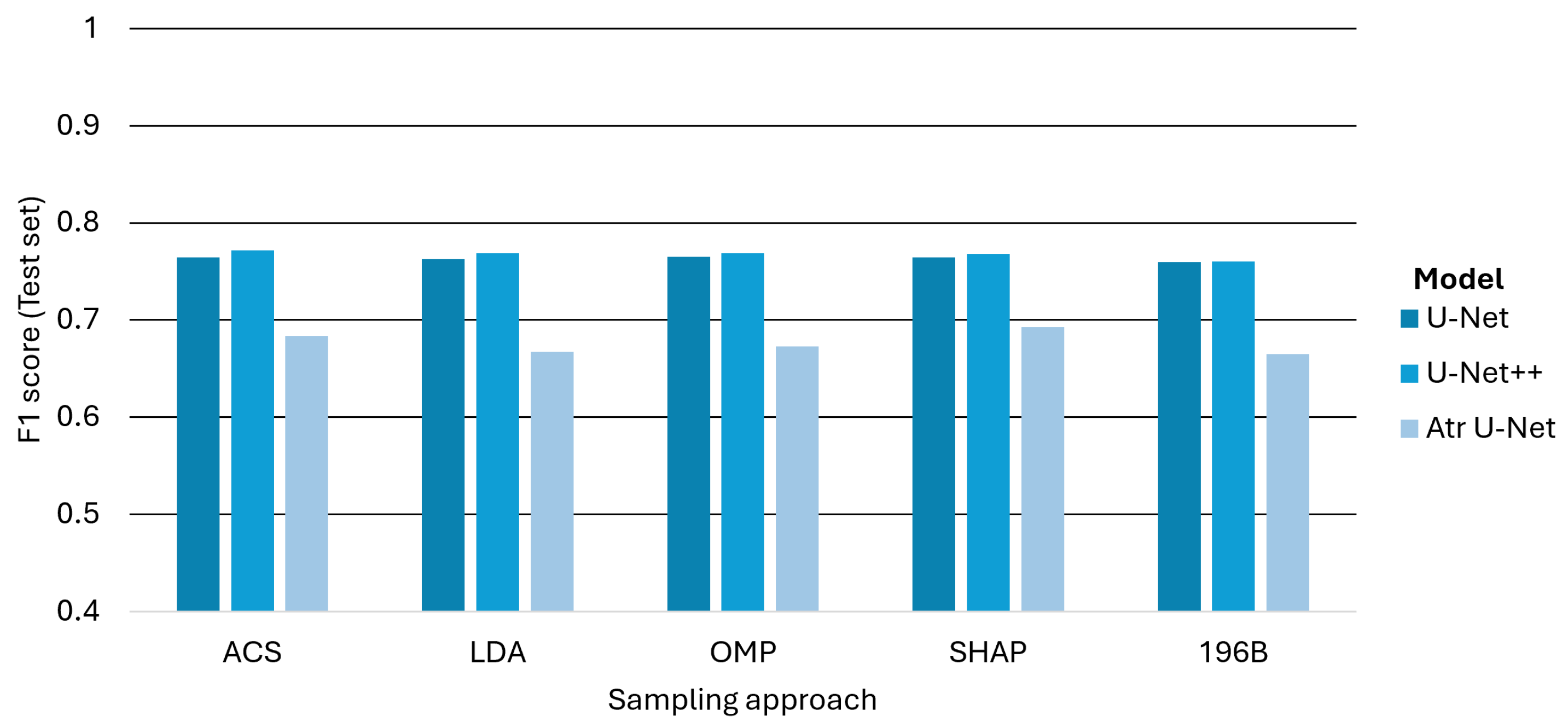
Figure 11 presents the classification performance of each model across five different band selection approaches. The results, averaged across all classes, show that the Unet_PP architecture delivers strong overall performance, achieving the highest mean F1-score of 0.77 when combined with ACS-derived subsets. This is particularly noteworthy since ACS reduces the spectral dimensionality from 196 to 60 bands (a 70% reduction), yet retains or even enhances predictive accuracy. Interestingly, SHAP achieves a much more compact representation (19 bands, i.e., over 90% reduction) and, when paired with all U-Net architectures, yields competitive results compared with full-spectrum models. These findings underscore the operational potential of compact band representations for large-scale agricultural monitoring.

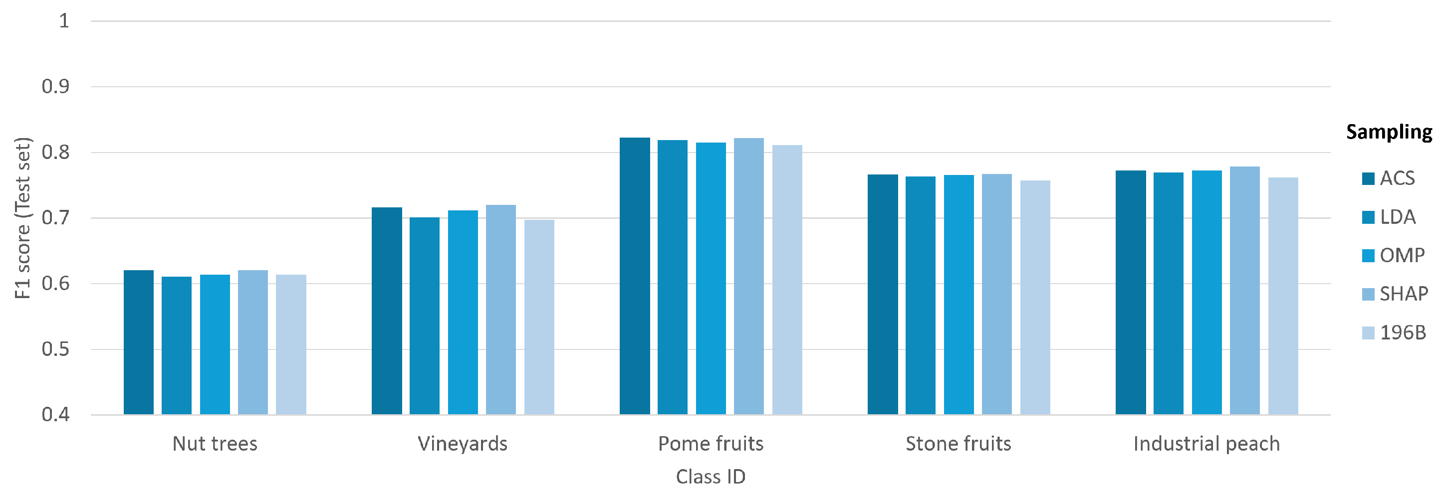
Figure 12 demonstrates the impact of band selection on the classification performance for each investigated class. The results reveal a significant variation in F1-scores across the different classes, with the separability of the classes being a more dominant factor than the choice of band selection strategy. Notably, the Stone fruits and Industrial peach classes consistently yield high F1-scores, whereas the Nut trees and Vineyards classes prove to be more challenging, achieving lower scores. Furthermore, within each class, the performance across the different band selection methods (ACS, LDA, OMP, SHAP, and 196B) is remarkably consistent, with only minimal variations. This finding underscores that the intrinsic nature and distinctiveness of the target classes are the primary determinants of classification success in this experimental setup.

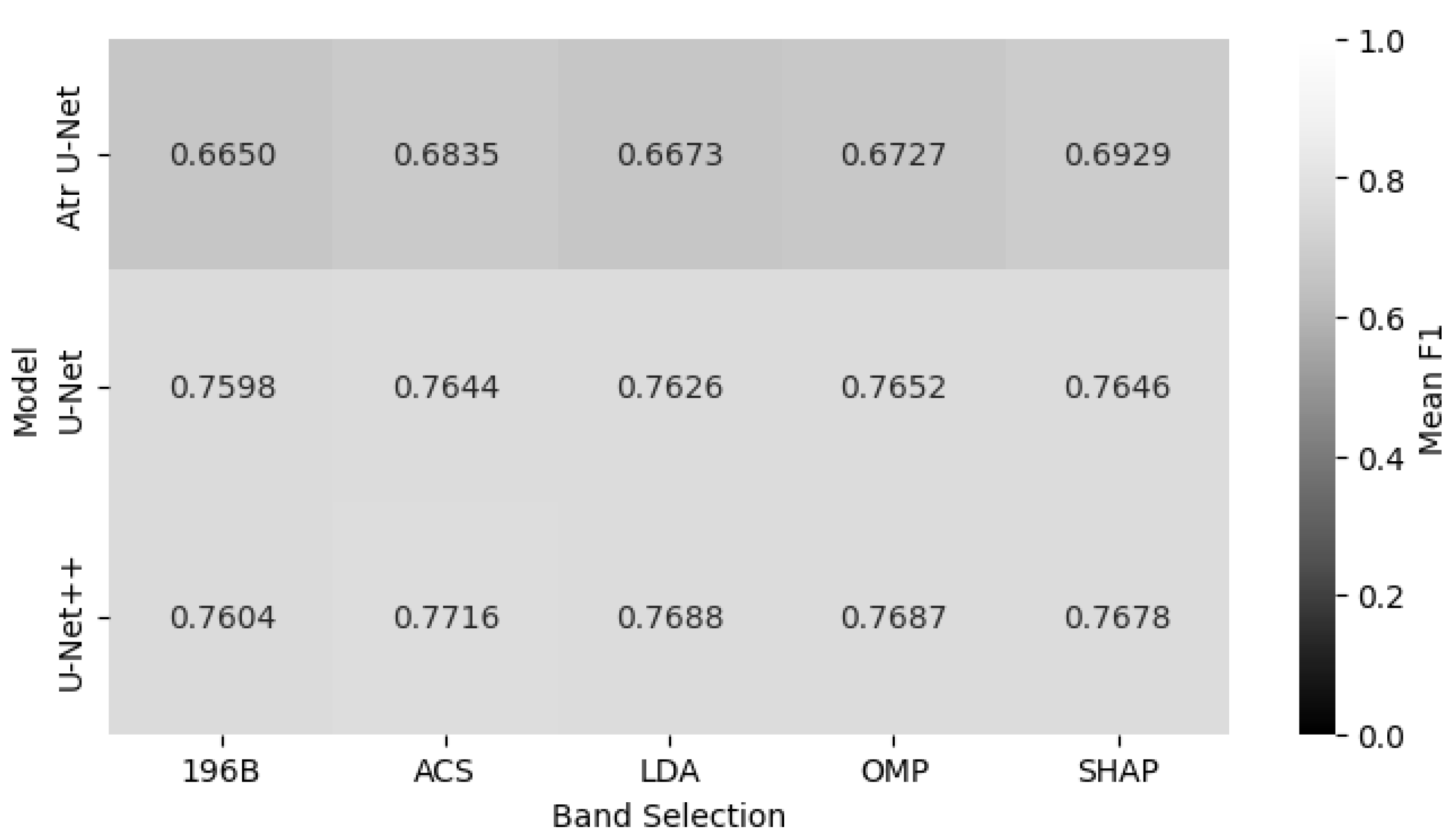
Figure 13 provides a comprehensive overview of the average F1-scores for all investigated models and band selection scheme combinations. The results demonstrate that the U-Net++ architecture combined with the ACS band selection method constitutes the optimal overall scheme, achieving the highest mean F1-score of 0.7716. However, a more detailed analysis reveals the best band selection approach for each specific architecture. For the standard U-Net, the optimal performance is achieved with the OMP strategy, yielding an F1-score of 0.7652. The Atrous U-Net model performs best when paired with the SHAP method, although its F1-score of 0.6929 remains significantly lower than those of its counterparts, reinforcing its systematic underperformance. These findings underscore that while the choice of architecture is the primary determinant of overall performance, subtle gains can be achieved by optimizing the band selection strategy for each specific model.

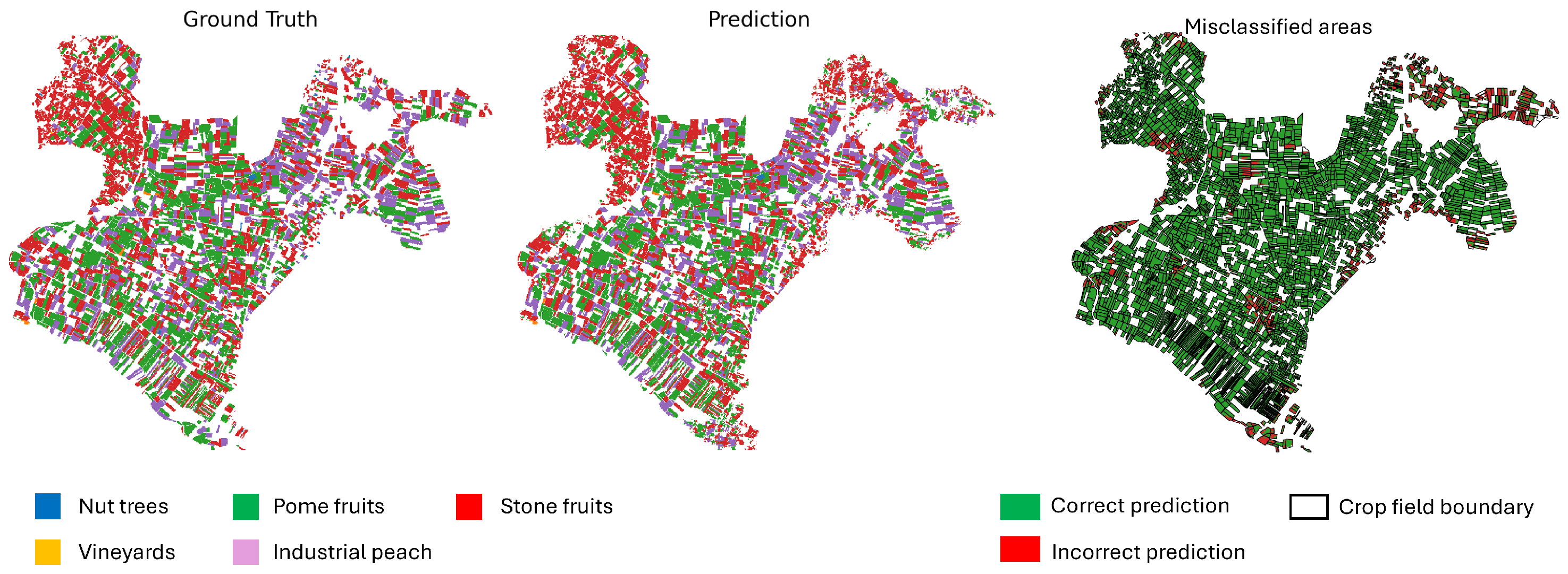
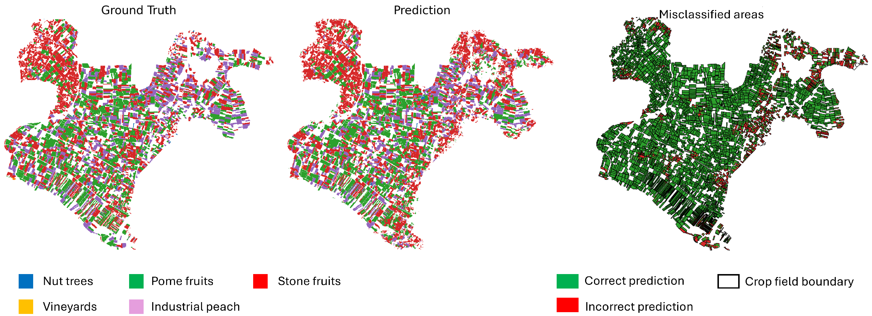
Figure 14, Figure 15 and Figure 16 provide a comparison between the ground truth and the model predictions. The left panel shows the annotated ground truth, while the center panel displays the model’s predictions across the test set. The right panel highlights misclassified pixels, where the prediction does not match the ground truth. Dominant perennial crop categories—including nut trees, pome fruits, and stone fruits—are represented using distinct color codes. The error map aids in identifying spatial patterns of misclassification, offering insight into areas where the model underperforms.

Overall, the experimental results highlight three key insights: (i) dimensionality reduction substantially improves efficiency without sacrificing accuracy, (ii) U-Net++ is generally robust but not universally superior, and (iii) the optimal configuration emerges from jointly selecting the architecture and the feature space. These findings set the stage for the broader interpretation provided in the discussion section.

3.5. Statistical Tests

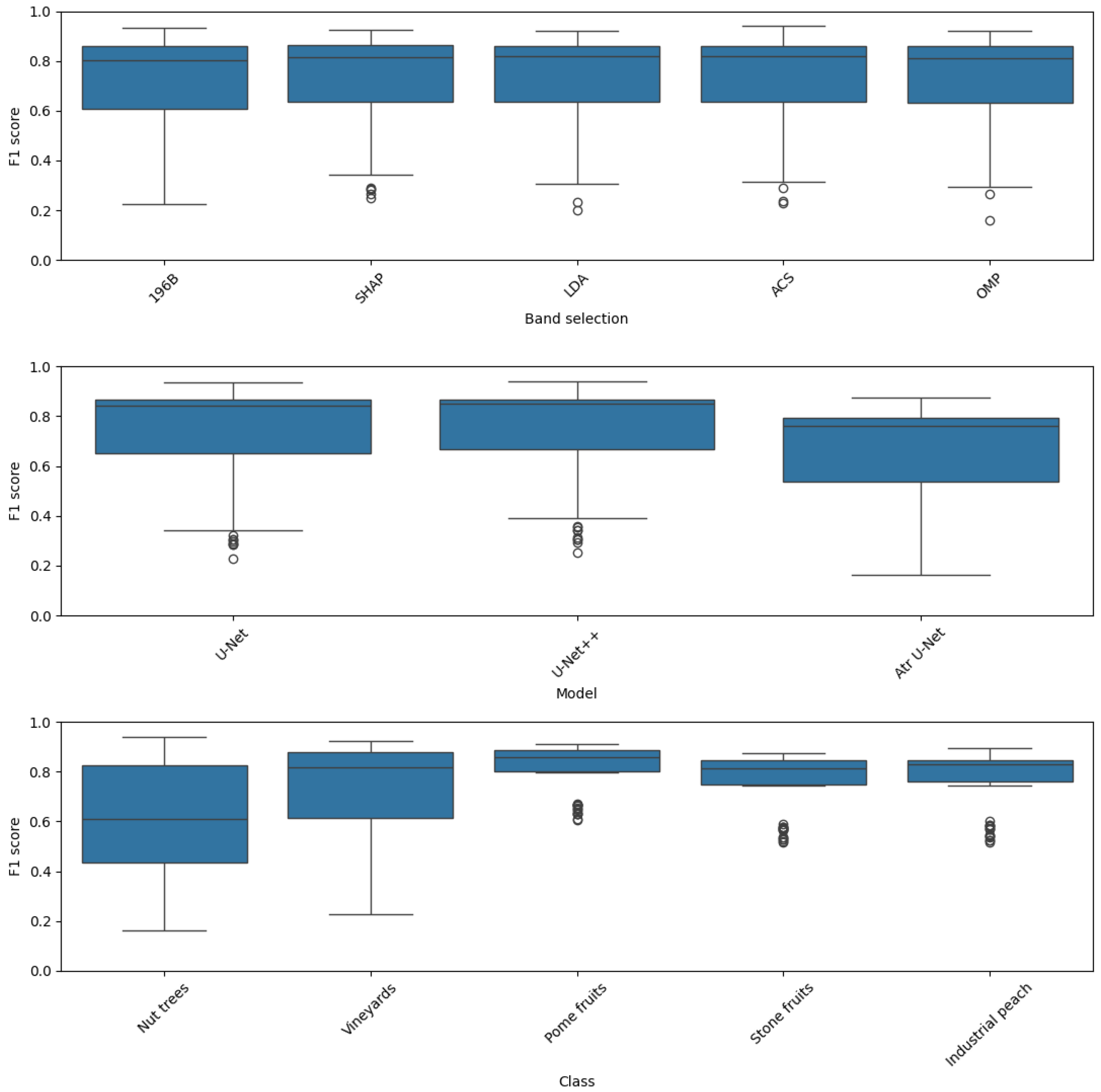
To assess the statistical significance of performance differences among the evaluated models, a comprehensive analysis was conducted based on the F1-scores computed on the test sets over the five holdout sets. Figure 17 illustrates the distribution of these scores using boxplots.

The top subplot, which illustrates the distribution across different band selection methods, suggests that this factor has a limited impact on overall performance, as the median F1 scores and interquartile ranges for all methods (196B, SHAP, LDA, ACS, and OMP) are very similar. In contrast, the middle subplot, which visualizes performance across the model architectures, provides strong evidence for a clear architectural hierarchy. The U-Net++ box plot is positioned highest with a tight distribution, indicating consistently superior performance, followed by the U-Net model. The Atrous U-Net model exhibits a significantly lower median and a wider spread, signifying its systematic underperformance. This analysis underscores that the choice of architecture is a far more impactful factor than band selection.

The influence of the target class, as shown in the bottom plot, has a peculiar behavior. The inherent separability of the classes appears to be a dominant factor, affecting F1 score distributions. The distributions for Pome fruits, Stone fruits, and Industrial peach are characterized by high median F1 scores and minimal spread, indicating these classes are consistently easy to classify. In contrast, the boxplots for Nut trees and Vineyards show significantly lower medians and much broader distributions, highlighting their inherent difficulty and the high variability in classification performance. In summary, the F1 score is most sensitive to the intrinsic properties of the class being identified, followed by the model architecture, while band selection has a comparatively negligible effect on the overall outcome.

Despite the good overall performance of several deep learning models and/or band selection approaches, the proximity of their mean F1-scores makes it difficult to draw conclusions based on descriptive statistics alone. Therefore, a formal statistical testing framework was adopted to rigorously examine whether the observed differences are statistically significant.

Based on the preliminary statistical evaluation of the F1-score data, the assumptions for a parametric analysis of variance (ANOVA) were assessed. The Shapiro–Wilk test for the normality of residuals yielded a p-value of 0.0000, which is significantly less than the typical $\alpha =0.05$ threshold. This result rejects the null hypothesis of normality, indicating that the residuals are not normally distributed. In contrast, Levene’s test for the homogeneity of variances produced a p-value of 0.9811, which is well above the significance level, thus satisfying this assumption. Given that the fundamental assumption of normality was violated, the use of a parametric test like ANOVA would be inappropriate. Therefore, a non-parametric alternative, such as the Kruskal–Wallis test, is more appropriate.

The Kruskal–Wallis test was conducted to assess whether different band selection strategies had a significant effect on the F1 performance. The results indicated no statistically significant differences among groups ($H=0.587$, $p=0.964$). Consistently, post-hoc pairwise comparisons using the Mann–Whitney U test with Holm correction confirmed the absence of significant differences across all pairings (

Table 10. Post-hoc pairwise comparisons for the Band Selection factor (Mann–Whitney U tests with Holm correction). No significant results were observed.

Group 1	Group 2	U	p-Value (Raw)	p-Value (Holm)
196B	SHAP	2628.0	0.489	1.000
196B	ACS	2664.0	0.578	1.000
SHAP	OMP	2928.0	0.666	1.000
SHAP	LDA	2917.0	0.696	1.000
196B	OMP	2735.0	0.772	1.000
ACS	OMP	2887.0	0.781	1.000
196B	LDA	2739.0	0.784	1.000
LDA	ACS	2742.0	0.792	1.000
SHAP	ACS	2847.0	0.898	1.000
LDA	OMP	2798.0	0.958	0.958

). This suggests that the choice of band selection method did not substantially influence the model performance.

This finding aligns with the preliminary observations from the boxplot analysis, which visually suggested a high degree of similarity in the performance distributions of the different band selection methods. Consequently, post-hoc pairwise comparisons were not necessary, as the omnibus test showed no significant overall effect. The results confirm that, within the context of this study, the choice of band selection strategy does not exert a significant influence on the models’ classification performance.

The Kruskal–Wallis test revealed statistically significant differences among the model architectures ($H=62.190$, $p<0.001$). Post-hoc pairwise Mann–Whitney U tests with Holm correction (

Table 11. Post-hoc pairwise comparisons for the Model factor (Mann–Whitney U tests with Holm correction).

Group 1	Group 2	U	p-Value (Raw)	p-Value (Holm)
U-Net++	Atr U-Net	11,792.0	$3.40\times {10}^{-12}$	$1.02\times {10}^{-11}$
U-Net	Atr U-Net	11,636.0	$2.27\times {10}^{-11}$	$4.55\times {10}^{-11}$
U-Net	U-Net++	7814.0	0.999	0.999

) indicated that the Atrous U-Net significantly underperforms compared with the U-Net++ and the standard U-Net ($p_{\mathrm{Holm}}<0.001$ in both cases). No significant differences were observed between the U-Net++ and the standard U-Net ($p_{\mathrm{Holm}}\approx 1.000$).

The Kruskal–Wallis test indicated statistically significant differences among crop classes ($H=39.740$, $p<0.001$). Post-hoc pairwise Mann–Whitney U tests with Holm correction (

Table 12. Post-hoc pairwise comparisons for the Class factor (Mann–Whitney U tests with Holm correction).

Group 1	Group 2	U	p-Value (Raw)	p-Value (Holm)
Nut trees	Pome fruits	1372.0	$6.21\times {10}^{-8}$	$6.21\times {10}^{-7}$
Pome fruits	Stone fruits	3962.0	$1.57\times {10}^{-5}$	$1.41\times {10}^{-4}$
Pome fruits	Industrial peach	3833.0	$1.26\times {10}^{-4}$	$1.01\times {10}^{-3}$
Nut trees	Industrial peach	1808.0	$1.61\times {10}^{-4}$	$1.13\times {10}^{-3}$
Nut trees	Stone fruits	1879.0	$4.53\times {10}^{-4}$	$2.72\times {10}^{-3}$
Nut trees	Vineyards	2144.0	$1.20\times {10}^{-2}$	0.060
Vineyards	Pome fruits	2212.0	$2.41\times {10}^{-2}$	0.096
Vineyards	Stone fruits	3143.0	0.215	0.645
Stone fruits	Industrial peach	2598.0	0.421	0.842
Vineyards	Industrial peach	2989.0	0.508	0.508

) revealed that Nut trees, Pome fruits, and Industrial peach exhibited consistently higher performance differences compared to other classes. In particular, Nut trees vs. Pome fruits, Pome fruits vs. Stone fruits, and Pome fruits vs. Industrial peach all showed highly significant differences ($p_{\mathrm{Holm}}<0.01$). Conversely, comparisons involving Vineyards or Stone fruits vs. Industrial peach did not reach significance.

The statistical analysis results, combined with the outcomes of Section 3.4, validate the importance of carefully selecting both the architecture and dimensionality-reduction strategy in hyperspectral classification tasks. The statistical evidence further supports the robustness of the proposed methodology and the reliability of the performance comparisons made in this study.

4. Discussion

The comparative evaluation demonstrates that both network architecture and spectral representation decisively shape hyperspectral crop classification performance. U-Net++ frequently yields the most robust results, particularly when coupled with ACS-based subsets. Yet, regardless of the band selection scheme, U-Net++ performs marginally better than its counterparts. These findings underscore the importance of considering architecture–feature space interactions rather than attributing performance differences to architecture alone.

An equally important outcome is the demonstration that judicious dimensionality reduction enhances parsimony without compromising predictive accuracy. In particular, ACS and SHAP methods reduce the spectral dimensionality by over 50% while preserving nearly all discriminative power. The advantages of processes involving dimensionality reduction [40] or band selection [45] have been reported in similar studies. Beyond computational savings, this compactness promotes interpretability and operational viability, particularly in large-scale monitoring pipelines.

The strict parcel-based spatial holdout with buffer enforcement addresses the pervasive risk of spatial autocorrelation, ensuring unbiased performance estimation. The appropriate process for sample selection remains an important research topic [46]. This methodological rigor strengthens the validity of our reported accuracies and enhances comparability with future work. The finding that class separability (e.g., industrial peach vs. nut trees) strongly influences classification accuracy further illustrates that the challenge lies not only in architectural design but also in the inherent spectral properties of the target crops.

At the same time, several limitations remain that define natural directions for future research. The reliance on a single EnMAP acquisition constrains temporal generalization, although the chosen site includes diverse perennial fruit crops with high intra-class variability. Extending this framework to multi-temporal EnMAP stacks will enable insights into seasonal crop dynamics and improve generalizability across growing seasons, as already demonstrated in the work of [47].

Similarly, while our focus on U-Net variants allowed for controlled architectural comparisons, evaluating lightweight or edge-optimized segmentation models would further strengthen the operational applicability of the framework, particularly in resource-constrained environments such as UAVs or mobile ground platforms. The current research advocates favorably towards such approaches [48].

Overall, this study clarifies the conditional strengths of U-Net variants and highlights the operational value of compact spectral inputs, while also identifying methodological extensions that can further enhance the scalability and transferability of hyperspectral crop classification.

5. Conclusions

This study systematically compared U-Net, U-Net++, and Atrous U-Net architectures for hyperspectral crop classification using EnMAP satellite imagery, in combination with four dimensionality-reduction strategies. The results demonstrate that classification performance is governed not only by network design but also by the interaction with the input feature space. U-Net++ consistently achieved high performance, particularly with ACS-selected bands. Nevertheless, the marginally different performance of these combinatorial approaches highlights the necessity of aligning model architecture with spectral representation rather than assuming universal superiority of any single network.

Equally significant is the demonstration that compact spectral subsets can sustain competitive accuracy. Both ACS and SHAP methods achieved 70% and 90% band reduction, while preserving classification performance close to the full-spectrum case, with the U-Net++, for which the ACS configuration reached a mean F1-score of 0.77. This efficiency gain reduces computational burden, improves interpretability, and underscores the practical viability of dimensionality reduction in operational agricultural monitoring. Collectively, these results establish a reproducible framework for precision crop mapping, balancing methodological rigor with real-world applicability.