Article

Modeling How the Different Parts of the Immune System Fight Viruses

by
Benito Chen-Charpentier
Department of Mathematics, University of Texas at Arlington, Arlington, TX 76019, USA
Algorithms 2025, 18(9), 544; https://doi.org/10.3390/a18090544
Submission received: 3 July 2025 / Revised: 18 August 2025 / Accepted: 21 August 2025 / Published: 29 August 2025

Abstract

Viruses cause a large number of diseases. After penetrating into a host, the virus starts infecting healthy cells. Then it uses the RNA or DNA of the cell to replicate and afterward it explodes the infected cell, letting out many copies of the virus that can infect new cells. The innate and adaptive parts of the immune system defend the body by eliminating both the free viruses and the infected cells. Neutrophils, macrophages, natural killer cells, helper T cells (CD4+) and cytotoxic T lymphocytes (CD8+) are among the participating immune cells. The interactions are complex and not fully understood. In this paper, we present and study three mathematical models based on ordinary differential equations of virus and immune system interactions with different complexities, and also introduce possible treatments. We discuss the advantages and disadvantages of each model. We do global sensitivity analysis and numerical simulations. Finally, we present conclusions including comments about the complexity of mathematical models.

1. Introduction

There are many diseases in humans, animals, and plants that are caused by viruses. In humans, viruses cause the common cold (Rhinovirus/Enterovirus, Respiratory Adenoviruses), flu (Influenza), COVID-19 (SARS-CoV-2), measles, hepatitis (A, B, and C), AIDS (Human Immunodeficiency Virus), and many others. Some are also found in animals, such as rabies. The effects of a viral infection can vary from mild, as for the flu, to very serious and even deadly, as for COVID-19, AIDS, and Ebola. Viruses are very simple non-cellular entities. Each virus particle (or virion) consists of a nucleic acid core (RNA or DNA), an outer protein coating, and sometimes an outer envelope [1]. Once the virus is inside an organism, it replicates by penetrating into a healthy cell and using the cell’s RNA or DNA to make copies of its genetic material, and, finally, it bursts the cell, producing many new virions. For many viral infections there are vaccines and antivirals that can be used to prevent and fight the infection. Vaccines are usually administered as prevention before the individual gets the disease, training the immune system to recognize and fight the virus. Antivirals are medications that reduce the severity and the duration of the infection. Antivirals do not kill the virus directly, but usually reduce, and even suppress, the virus’ ability to infect and replicate in the organism cells [2]. The first defense to prevent a viral infection in a human or animal host are the physical barriers such as the skin and cilia in the respiratory tract. But viruses can overcome these barriers. Once the virus is inside the body, the innate immune system responds with inflammation, virus phagocytosis, and secretion of cytokines, chemical factors, and proteins [1]. The innate immune system is non-specific and responds to the presence of any pathogen (virus or bacteria) and even of any debris. The next response is by the adaptive immune system which takes longer to act than the innate system but is more specific and also has memory. There are many different immune system cells, cytokines, and other chemical factors involved. The processes are complex. Within-host, or within-body, mathematical models of viral infections can help understand the very complex interactions between the different cells, chemical substances, and virions. The models complement the experimental and clinical work and can help in determining treatment options. A basic within-body viral infection mathematical model consists of three populations: susceptible cells, infected cells, and virions. Their interactions and rates of change are given by ordinary differential equations (ODEs) [3,4,5]. This model has been widely used but it neglects important processes. One method of improvement is to add effector cells to kill the infected cells [6,7] or to kill the virus [8,9]. Both processes are included without giving explicit equations for the immune system in [10]. Additional cells of the immune system are included in [11,12,13]. There are other interactions that have been observed for some virus infections. One such interaction is when the virus is also transmitted by cell-to-cell contact [14,15]. Delays due to the virus replication time are also discussed in many papers including [16,17,18]. Models that include the effects of treatment are studied in [19,20,21,22]. Ref. [23] has a review of different types mathematical models involving immune cells. In the present paper we introduce and analyze a new within-host virus infection model, based on ordinary differential equations. It includes healthy cells, infected cells, virions, and several innate and adaptive immune system cells. It also has cell-to-cell infection. Two simpler previously published models are included in the study. We give advantages and disadvantages of each model for comparison purposes, taking into account the quote “Everything should be made as simple as possible, but not simpler”, often attributed to Einstein. The models are presented and studied in Section 2. Section 3 contains numerical simulations for a model of hepatitis B which are performed first with no treatment and then with treatment. Finally, there is a discussion followed by the conclusions in Section 4.

2. Materials and Methods

The first within-host virus infection model we study, named Model 1, is very simple. It is based on ODEs using the usual assumptions that the populations are continuous and well mixed. It also assumes that the interactions are of mass action type, which assumes that the number of contacts between two different populations is proportional to the product of the number of individuals in each of the populations. Mass action kinetics is a simplification. It is used to avoid adding more parameters to the models. Other modeling possibilities for the interactions include using Holling type II functions [24] if one population of the two interacting is much greater than the other, or Beddington–DeAngelis functions [25] if the proportions between the interacting populations may change significatively with time, or Hill-type or Michaelis–Menten kinetics. This model only includes three populations: susceptible cells, infected cells, and virus particles (virions) [3,4,5]. It is based on the following hypotheses. In the absence of virus, susceptible (or healthy) cells are recruited and die naturally. In a viral infection, these cells may become infected by the invasion of a virus particle. The virus replicates inside the cell and then the cell membrane breaks and a certain number of virions are released. These free virions can infect other susceptible cells or die. This death process is not specified but it is implied to include natural death and elimination by the immune system. All parameters of the model are deterministic even though in real life they have variability. This is also a common simplification. Deterministic models assume that you accurately know the values of the parameters and the present state of the system, and, therefore, can predict the system future. For models in mathematical biology, this is not true due to variation of the populations, measurement errors, incomplete data, and many other reasons. Stochastic models can better deal with the uncertainties and produce a range of possible outcomes. Deterministic models are easier to understand and implement, are computationally faster, and easier to analyze. Models are usually first developed as deterministic models and then made more realistic by including stochasticity. See [26] for a comparison of deterministic and stochastic approaches in biochemical interaction. The parameters are also non-negative. The system of equations that describes Model 1 is as follows:
d x d t = λ μ x x β x v d y d t = β x v μ y y d v d t = B μ y y μ v v .
Here, x , y , and v are the concentrations of susceptible cells, infected cells, and virions, respectively. λ is the recruitment rate of new susceptible cells, μ x is their natural death rate, β is the infection rate, μ y is the elimination rate of infected cells by the virus, B is the number of virions produced per infected cell, and μ v is the death rate of virions due to the immune system and natural elimination.
A simple way of adding the process of effector cells eliminating infected cells, but without adding the effector cells explicitly, is to change the virus equation into
d v d t = B μ y ( 1 f e ) y μ v v ,
where f e is the fraction of infected cells killed by the immune system. It has the advantage of not adding more equations, but it assumes that the elimination rate of infected cells by the immune system is constant and independent of the number of effector cells. We will not consider this approach.
The solutions x ( t ) , y ( t ) , v ( t ) of Model 1 (system (1)) are non-negative and bounded above if true for the initial values x ( t 0 ) , y ( t 0 ) , v ( t 0 ) [27].
System (1) has two equilibrium points, the infection free equilibrium, or, if using the notation from epidemics, the disease free equilibrium (DFE):
x * = λ / μ x ,   y * = 0 ,   v * = 0 ,
and a chronic, or in the epidemic notation endemic equilibrium (CE):
x * = μ v / ( B β ) ,   y * = ( B β λ μ v μ x ) / ( B β μ y ) ,   v * = B λ / μ v μ x / β .
The most important question a within-body infection model can answer is whether the infection will disappear or turn chronic. This can be carried out by finding the eigenvalues of the linearized system evaluated at the infection free equilibrium point. But for Model 1, determining the sign of the real part of the eigenvalues is not straight forward. But it is not necessary to do so since the basic reproduction number (also called basic reproductive number) R 0 is a very useful index for this determination. It is the average number of newly infected cells generated by a single virus particle at the beginning of the infection process. For Model 1, it can be calculated directly as the product of the probability of having a new infected cell per susceptible cell, β , times the number of susceptible cells at the beginning of the process with only one virion, λ / μ , times the number of virus particles produced from the bursting of that infected cell, B, times the average lifetime of a virion, 1 / μ v . Therefore R 0 = β ( λ / μ x ) B / μ v . If R 0 > 1 , the number of virus particles increases, and the CE makes biological sense since all the populations are non-negative. If R 0 < 1 , the infection disappears and the DFE equilibrium is the only one that is non-negative. For more complex models, the calculation of R 0 from its definition is hard. But in order to determine if the infection will grow, it is only necessary to look if the infected compartments, y ( t ) and v ( t ) , grow. This is used in the the next generation matrix method [28,29] that is widely used to calculate the basic reproduction number in more complex models in epidemiology. Applying this method to Model 1, we need to consider the two infectious compartments, y and v. The right-hand side of the y equation has two parts, the transmission part f 1 = β v λ / μ x and the transition part v 1 = μ y y . For the v equation, the corresponding parts are f 2 = B μ y and v 2 = μ v v . The transmission matrix is
F = f 1 y f 1 v f 2 y f 2 v = 0 β λ / μ x B μ y y 0 .
And the transition matrix is
V = v 1 y v 1 v v 2 y v 2 v = μ y 0 0 μ v .
Therefore
F V 1 = 0 β λ μ v μ x B 0 .
The spectral radius of this matrix gives the basic reproduction number as produced by the next generation matrix method, R 0 N G = β ( λ / μ x ) B / μ v . While R 0 N G = 1 if and only if R 0 = 1 , they are not equal. Ref. [30] called R 0 N G the one generation basic reproduction number. But both predict a chronic state and both are used. Using the characteristic polynomial and the Routh–Hurwitz criterion is another possibility [31,32]. Applying it to the basic Model 1, the characteristic polynomial is
p ( r ) = r 2 + r ( μ v + m u y ) + μ v μ y B β μ y λ / μ x = r 2 + a 1 r + a 0 .
All the eigenvalues r are negative if and only if a 1 > 0 and a 0 > 0 . a 1 is always positive and a 0 > 0 if and only if 1 > B μ y β λ / μ x = R 0 . Therefore, R 0 > 1 implies that the DFE is locally asymptotically unstable so at least one of the eigenvalues of the linearized system about the DFE has positive real part and the infection is chronic.
A more complete analysis of Model 1 including positivity and boundedness of the solutions is performed in [33].
Model 1 can be made more realistic by incorporating more processes that have been observed. First is the inclusion of effector cells of the immune system that eliminate infected cells and virions. Second is the addition of cell-to-cell transmission. This is based on the results in [15,18,34,35] and used in [27]. In this model, denoted by Model 2, there is only one type of immune cell which is left unspecified. The equations of Model 2 are
d x d t = λ μ x x β x v β x y x y d y d t = β x v + β x y x y β e y y e μ y y d v d t = B μ y y β x v β e v v e μ v v d e d t = s + α 1 y β y e y e β v e v e μ e e .
In Model 2, x , y , v, and e are the concentrations of susceptible cells, infected cells, virions, and effector cells, respectively. As in Model 1, λ is the recruitment rate of new susceptible cells, μ x is their death rate, β is the infection rate of susceptible cells by free floating virions, μ y is the elimination rate of infected cells by the virus, B is the number of new virions produced per infected cell, and μ v is the death rate of virions. Now this death rate is the natural death rate of the virions. In addition, susceptible cells can also be infected by direct contact with an infected cell at a rate of β x y ; effector cells eliminate infected cells at a rate of β e y ; free virus particles penetrate into susceptible cells at a rate of β ; and effector cells are recruited at a constant rate of s but there is an additional recruitment depending on the number of infected cells y at a rate of α 1 . Furthermore, effector cells eliminate infected cells and virus particles at rates of β y e and β v e , respectively. Finally, effector cells die naturally or are eliminated by the body at a rate of μ e . All parameters are non-negative. Since Model 2 has more parameters and variables, the naming specially of the parameters starts being an issue. The infection rate of susceptible cells by virions is denoted by β as is commonly performed. The infection rate by contact between a healthy cell x and an infected cell y is denoted by β x y with x y as a sub-index to help remember that it is the coefficient of the interaction between x and y. This is similar for β y e and β v e . The death rates μ also have sub-indices to indicate the type of cell it refers to. This notation is also used later for Model 3.
It is also possible to show that the solutions of Model 2 are bounded and non-negative [27].
Model 2 still has two steady states, the disease or virus free equilibrium DFE,
x * = λ / μ x ,   y * = 0 ,   v * = 0 ,   e * = s / μ e ,
and a chronic or endemic equilibrium which can be calculated in close form but its expression is complicated. For the stability of the DFE, the eigenvalues of the linearized system can be found exactly but are not useful for general values of the parameters. But R 0 or an equivalent index can be used to see if there is a chronic infection. The new generation matrix method gives
R 0 N G = β x y x * 2 μ y + 2 β e y e * + 4 B x * β μ y ( β e y e * + μ y ) + β x y 2 x * ( β e v e * + μ v + β x * ) ( 2 β e y + μ y ) ( β e v e * + μ v + β x * ) .
An equivalent index can be found by looking at the characteristic polynomial of the infected compartments linearized about the DFE, and using the Routh–Hurwitz criterion
r 2 + r ( β e y e * + β e v e * + μ v + μ y + β x * β x y x * ) + ( β e v β e y ( e * ) 2 + β e y μ v e * + β e v μ y e * + μ y μ v + β β e y e * x * β e v β x y x * e * + β μ y x * β x y μ v x * B β μ y x * β β x y ( x * ) 2 ) = r 2 + a 1 r + a 0 .
So for the infection to persist a 1 > 0 which is true in practice since β and β x y are of the same order, and for a 0 < 0 we need
B β μ y x * + β e v β x y x * e * + β x y μ v x * + β β x y ( x * ) 2 β e v β e y ( e * ) 2 + β e v μ y e * + μ y μ v + β β e v e * x * + β μ y x * = R 0 R H > 1 .
Writing the characteristic equation as F ( r ) = r 2 + a 1 r = a 0 = G ( r ) and requiring that G ( 0 ) > 0 , we get the same index.
But it is not realistic to consider only one cell type from the immune system since they have different jobs and act at different times. The elimination of the free virions is performed by both the innate and adaptive immune systems while the elimination of the infected cells is carried out mostly by the adaptive system. The innate system acts first and then recruits the adaptive system. Herbert in [36] lists neutrophils and natural killer cells as the most important innate cells in fighting virus infections while natural killer T cells are possibly relevant. For the adaptive immune system he has B or plasma cells, cytotoxic T lymphocytes CD4+, and cytotoxic T lymphocytes CD8+. He mentions several signaling cytokines and factors only the antibodies as elimination agents. He briefly mentions macrophages but other authors state that they play very important roles [37,38]. For relevant immune processes, see also [39,40,41]. Therefore, the chosen variables for the third model, denoted vy Model 3, are as follows: x susceptible cells, y infected cells, v virions, N neutrophils, m macrophages, K natural killer cells, C 4 CD4+ cells, P plasma cells, C 8 CD8+ cells, and a antibodies. Also, see [9,42,43]. To avoid adding even more states we will not include the signaling cytokines, and simply assume that their amount is proportional to the cell or interaction producing it. For example, natural killer cells produce interferon I F N γ to activate CD4+ cells, but we consider that the natural killer cells activate CD4+ cells. The model is based on the following hypotheses [42,43,44]: no infection, susceptible cells, neutrophils, macrophages, and antibodies are recruited at a constant rate and die at a linear rate; susceptible cells are infected by contact with a virion or with an infected cell; infected cells grow as susceptible cells become infected, are eliminated by macrophages, natural killer cells and CD8+ cells and also die from bursting; free floating virions grow after replicating inside an infected cell, and decrease by entering a susceptible cell by being eliminated by neutrophils, macrophages, and antibodies, and by natural dead; neutrophils are also recruited by the presence of virions; macrophages are also recruited by the presence of infected cells and eliminated after engulfing an infected cell or a virion; natural killer cells are activated by macrophages and can die; CD4+ cells are activated by natural killer cells and can die; plasma cells are activated by CD4+ cells and die; CD8+ cells are activated by CD4+ cells and die; antibodies are also produced by plasma cells and are also eliminated after destroying a virion. Natural killer, CD4+, CD8+ and plasma cells may already be present but only the activated ones counteract the infection.
d x d t = λ μ x x β x v β x y x y d y d t = β x v + β x y x y β m y m y β K y K y β C 8 y C 8 y μ y y d v d t = B μ y y β x v β a v a v β N v N v μ v v d N d t = s N + k N y μ N N d m d t = s m μ m m + k m y y β y m m y β v m m v d K d t = k K m μ K K C 4 d t = k C 4 K μ C 4 C 4 d P d t = k P C 4 μ P P C 8 d t = k C 8 C 4 μ C 8 C 8 d a d t = k a + k a P P β v a a v μ a a .
The parameters not included in the previous Model 2 are as follows: β m y , the elimination rate of infected cells by macrophages; η K y , the elimination rate of infected cells by natural killer cells; β C 8 y , the elimination rate of infected cells by CD8+ cells; β a v the elimination rate of virions by antibodies; β v m , the elimination rate of virions by macrophages; β N v , the elimination rate of virions by natural killer cells; s N the recruitment rate of neutrohils in the absence of infection, k N , the recruitment rate of neutrophils due to the presence of the virus; μ N , the death rate of neutrophils; s m , the recruiting rate of macrophages in the absence of infection; k m y , the replenishing rate of macrophages due to infected cells; μ m , the death of macrophages; β y m , the elimination of macrophages due to engulfing an infected cell; k K , the activation rate of natural killer cells; μ K , the deactivation rate of natural killer cells; k C 4 , the activation rate of CD4+ cells; μ C 4 , the deactivation rate of CD4+ cells; k P , the activation rate of plasma cells; μ P , the deactivation rate of plasma cells; k C 8 , the activation rate of CD8+ cells; μ C 8 , the deactivation rate of CD8+ cells; k a , the production rate of antibodies in absence of an infection; k a P , the production rate of antibodies by activated plasma cells; μ a , the elimination rate of antibodies; β v a , the elimination rate of antibodies after reacting with a virus. All the new parameters are non-negative.
There are some mathematical models that consider different types of immune cells [11,13,21] but none has the same immune cells that we do and are based on different experimental results.
The analysis that can be performed of Model 3 is more limited. Similar methods as those used in [33,45] and many others can in principle be applied to find the existence, uniqueness, boundedness, and positivity of the solutions, and to find the equilibrium solutions and their stability. But the number of equations makes the analysis very hard or even intractable. The DFE can still be found in closed form but Mathematica [46] failed to find other equilibrium states. The DFE is as follows: x * = λ / μ x ,   y * = 0 ,   v * = 0 ,   N * = s N / μ N ,   m * = s m / μ m ,   K * = k K m * / μ K ,   C 4 * = k C 4 K * / μ C 4 ,   P * = k P C 4 * / μ P ,   C 8 * = k C 8 C 4 * / μ C 8 ,   a * = ( k a + k a P P * ) / μ a . s m 0 assumes that even with no infection there are macrophages and the other immune cells recruited by macrophages present. But it may only be true for certain viral diseases. We will take s m = 0 .
Mathematica also failed in determining the eigenvalues of the linearized system evaluated at the DFE. The basic reproduction number can still be calculated using the next generation matrix method. But the formula is several lines long and not useful except when the numeric values of the parameters are given. For numeric values of the parameters, simulations can give trajectories leading to steady solutions that are stable since they have truncation and round-off errors.
Model 3 is better from the modeling point of view since it includes more types of cells and interactions. But the analysis that can be completed is much more limited. It depends on many parameters, many of which are not given in the literature. Furthermore, the model is harder to understand.
There are several different types of antiviral treatments: some block receptors so the virions cannot enter into cells, and some lower the viral load by reducing the number of virus copies from an infected cell [1,47]. Vaccines boost the immune system by helping it recognize and remember given pathogens. They are usually administered before an infection, but they are sometimes administered after the infection for some slow-developing diseases, for example, rabies. So we will consider them separately from antivirals. Several authors include treatment in their models [19,48,49]. The effect of blocking receptors is performed by replacing the infection rate β in the equations by ( 1 ϵ ) β . The effect of reducing the viral load by multiplying the number of virions produced by a single cell B by ( 1 η ) . Both ϵ and η are between 0 and 1. To our knowledge, the effect of strengthening the immune system has not been introduced. We will model it by multiplying the elimination rate of virions and infected cells by effector cells by a large enough number so the immune system is better prepared and eliminates the infection very fast.We will also consider that there is a delay of several days τ v between the start of the infection and the administration and action of the antivirals since this is what happens in practice. For example, for the first type of antiviral, the factor is ( 1 H ( t τ v ) ϵ ) with H as the Heaviside function. The Heaviside function is the simplest one that will start the treatment at time t = τ v . It has previously been used by [19,20,21,22], where they assume that the antiviral is at full strength at t = 0 which is equivalent to using H ( 0 ) . It models only the starting time of the antiviral and its strength. Other functions such as sigmoids or arc-tangents can also be used but there is the question of how to choose how the fast the function increases. Also, for simplicity, we consider that the body does not eliminate the antiviral.
The equations for Model 1 with antiviral treatment included are (4)
d x d t = λ μ x x β ( 1 ϵ H ( t τ v ) ) x v d y d t = β ( 1 ϵ H ( t τ v ) ) x v μ y y d v d t = B ( 1 η H ( t τ v ) ) μ y y μ v v .
H is the Heaviside function.
Model 2 with treatment is given by (5)
d x d t = λ μ x x β ( 1 ϵ H ( t τ v ) ) x v β x y ( 1 ϵ H ( t τ v ) ) x y d y d t = β ( 1 ϵ H ( t τ v ) ) x v + β x y ( 1 ϵ H ( t τ v ) ) x y β e y y e μ y y d v d t = B ( 1 η H ( t τ v ) ) μ y y β x v β e v v e μ v v d e d t = s + α 1 y β y e y e β v e v e μ e e .
Model 3 with different immune cells with treatment is given by (6)
d x d t = λ μ x x β ( 1 ϵ H ( t τ v ) ) x v β x y ( 1 ϵ H ( t τ v ) ) x y d y d t = β ( 1 ϵ H ( t τ v ) ) x v + β x y ( 1 ϵ H ( t τ v ) ) x y β m y m y β K y K y β C 8 y C 8 y μ y y d v d t = B ( 1 η H ( t τ v ) ) μ y y β x v β a v a v β N v N v μ v v d N d t = s N + k N y μ N N d m d t = s m μ m m + k m y y β y m m y β v m m v d K d t = k K m μ K K C 4 d t = k C 4 K μ C 4 C 4 + s C d P d t = k P C 4 μ P P + s C C 8 d t = k C 8 C 4 μ C 8 C 8 + s C d a d t = k a + k a P P β v a a v μ a a .
For antivirals, s C is zero. The effects of a vaccine can be added by assuming that even in the absence of an infection, there is a base number of CD4+, CD8+, and plasma cells (given by s C 0 ) and that there is an increase the effectivity of CD8+ cells on infected cells and in the rate of the production of antibodies.
When studying any mathematical model with parameters, it is important to determine which parameters are the most influential. It is especially important to do so when there is a large number of parameters and interactions, and when the measured or estimated values of the parameters have large variations. Sensitivity analysis can determine which parameters have the largest effects on the solutions. Local sensitivity analysis is fast but it is valid only close to a given set of parameter values. But in mathematical biology the parameters usually have a large range of variation, so global analysis methods such as Sobol indices or E-FAST are the most widely used since they do not require a monotone dependence of the parameters on the states [50].

3. Results

For all models the numerical simulations give very useful information. We performed simulations without treatment and then with treatment. Since the data available has large variations due to differences in the individuals, errors, difficulties in the measurements, and different estimation methods, it is very important to do a global sensitivity analysis. This way the relative influence of each parameter on the solutions can be established. All the numerical simulations were performed using the julia software package, version v7.16.1 DifferentialEquations.jl [51]. In particular, we used the routine Rodas5P, which implements a fifth order A-stable stiffly stable Rosenbrock method for stiff equations [52] with a relative error of 1 × 10 6 and an absolute error of 1 × 10 10 .
For Model 1 the values of the parameters used are given in Table 1. Most studies of mathematical models within-body virus infection use generic values for the parameters. Even though we are not considering a specific virus disease, since the parameter values given in the literature are scarce, we use values of the parameters for the propagation of hepatitis B virus within the host presented in [34,35]. The number of patients studied in these two papers is very small and there is a large variability in the values. We multiplied β and B by a factor of 2 to obtain in the simulations a chronic equilibrium. For many individuals, viral infections like hepatitis B and C clear out. But for some, the infection persists. From the formula for R 0 , one way to increase R 0 is to increase β and B since these parameters have large variations in the data, as seen in [34]. But this is arbitrary and more research is needed to determine why in some individuals certain virus infections are chronic and not in others.
Figure 1 shows the simulation using Model 1 with the parameter values in Table 1. The values correspond to R 0 > 1 , so there is a chronic equilibrium. As can be observed, the number of infected cells and virions increases at first and then decays to a chronic steady value. That is, the viral infection is not cleared and instead remains persistent. Examples of virus infections that can be chronic are hepatitis B and C and HIV [53].
Table 2 has the parameter values used in Model 2. The parameters included Table 1 also have the same values. Model 1 is modified to include effector cells explicitly in [6,35,54] and the parameters involving the effector cells are taken from there. The infection rate, defined as the susceptibility to infected cells, is considered to be the same as by virions [15,18]. Although the experimental values of these two parameters estimated by data fitting have large variations, the assumption is that it takes the virion a lot less effort to leave a cell than to enter a cell. So the values of the two parameters can be taken to be numerically equal.
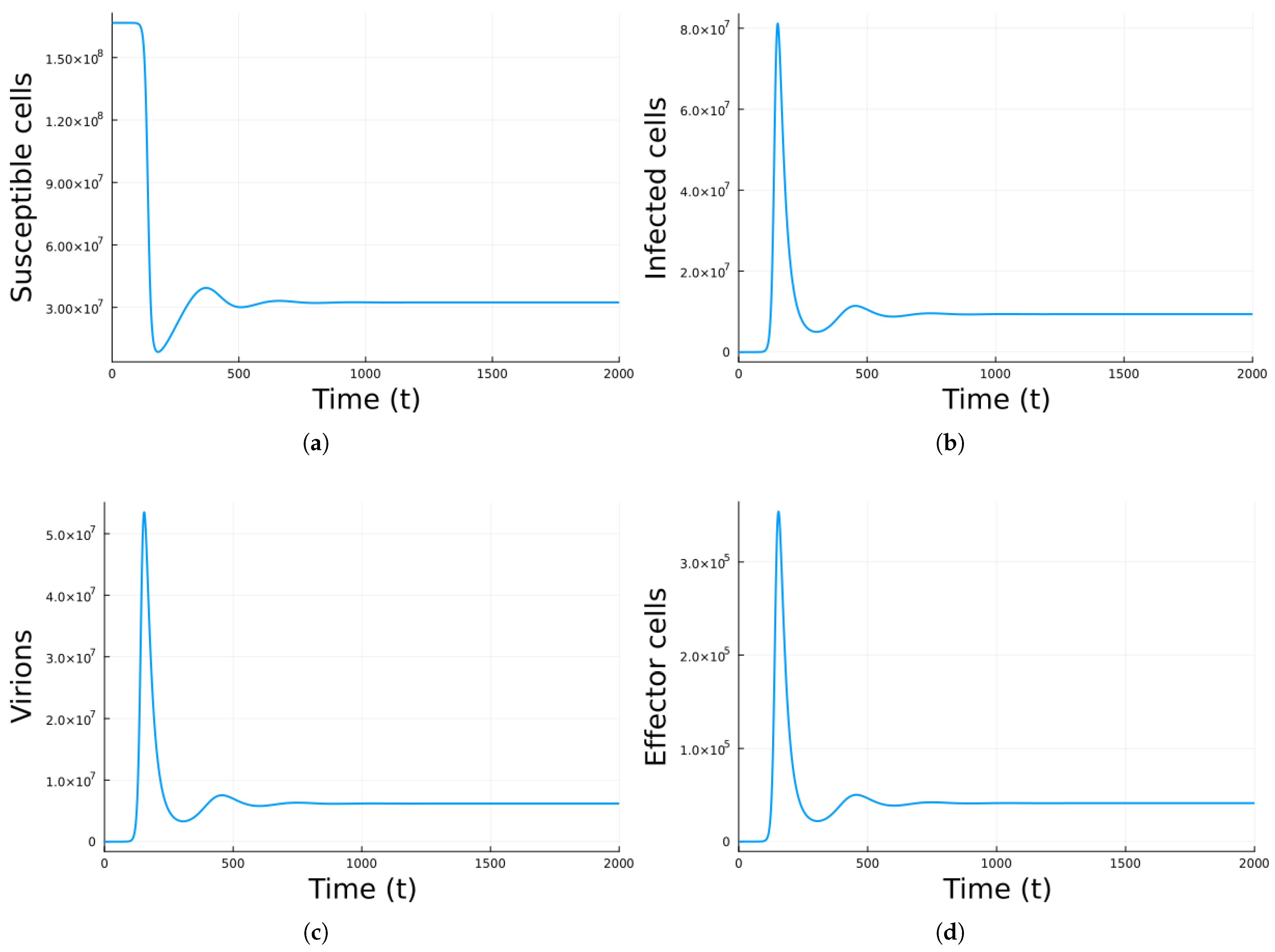
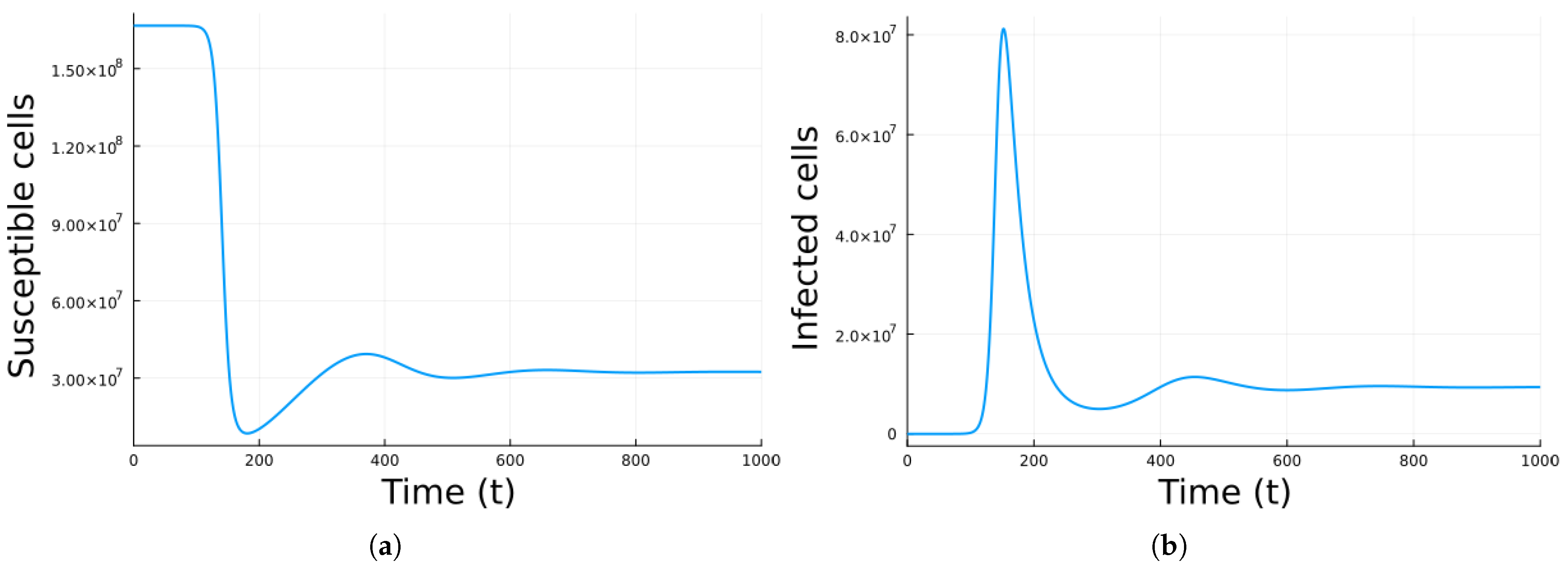
Figure 2 shows a numerical simulation using Model 2, with the parameter values in Table 2. The parameter values correspond to R 0 > 1 , so there is a chronic equilibrium. Initially, the number of infected cells, virions, and effector cells increases and then decays to the equilibrium state.
Table 3 has the parameter values for Model 3 without treatment. The recruitment rates and the death rates (calculated from the mean life spans) are based on the data in [55,56,57,58,59,60]. There are variations in the values presented by different authors for some parameters, with some given having large variation ranges [61,62,63]. So, representative values were used. But for others like the infection indices, we could not find experimental values, so we assumed that they were similar to the rates in Table 2 for effector cells.
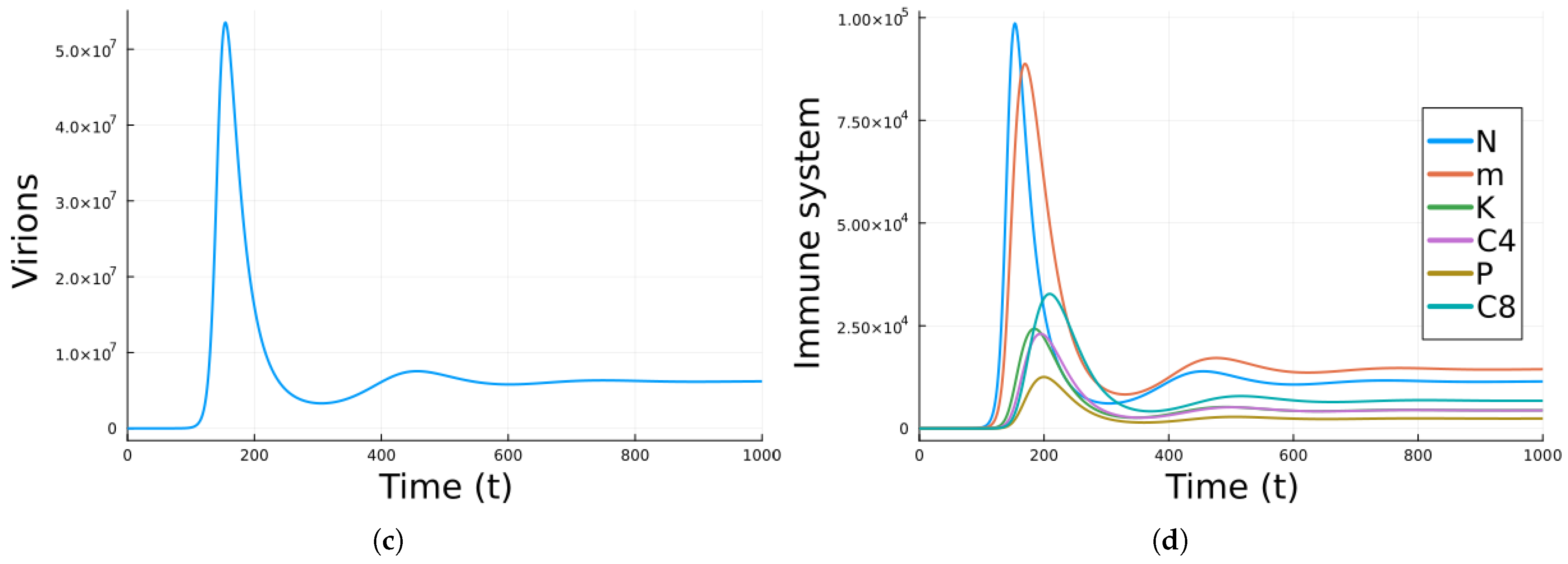
Figure 3 shows the results of a simulation using the parameters in Table 3. The values not included in Table 3 are in Table 2. The simulation gives a chronic equilibrium state since R 0 > 1 . All the populations, except the susceptible cells, start increasing and the decrease with slight oscillations to the equilibrium state. As expected, neutrophils grow first, then macrophages, and then the rest of the immune system cells.
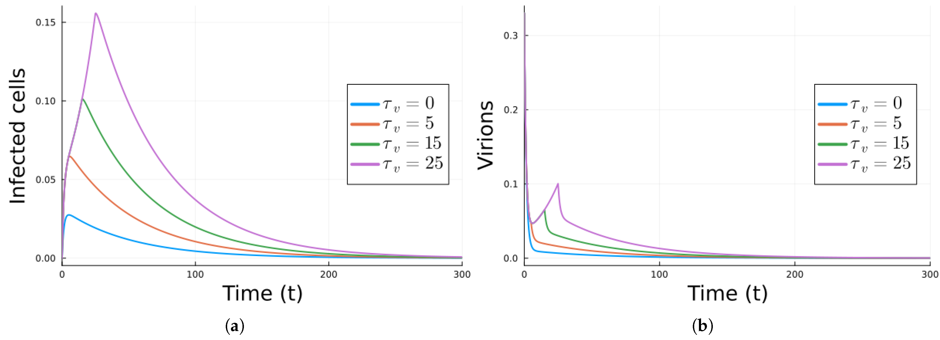
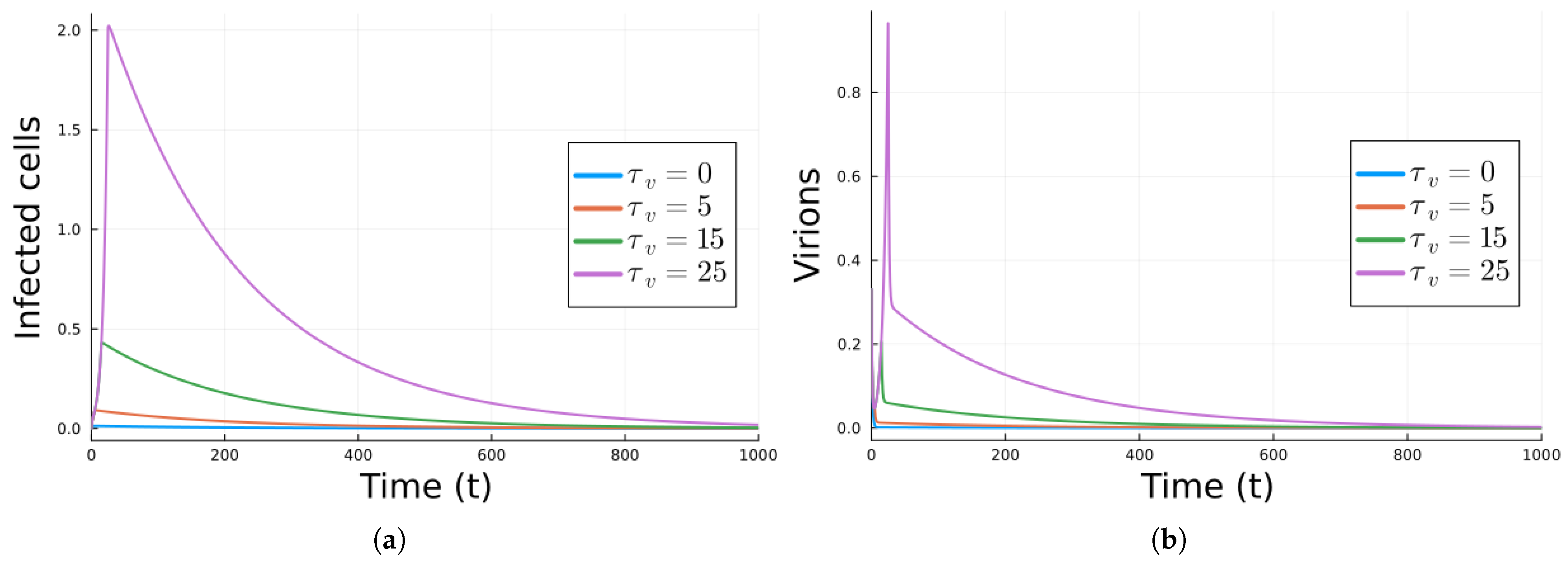
Next, we did simulations where we added antivirals. The equations for Model 1 with antivirals are Equation (4). The values of the parameters that model the antivirals are ϵ = 0.5 , η = 0.5 . With these values, the infection free equilibrium is stable ( R 0 < 1 ). To illustrate the effect of the delay in administering the antivirals, simulations were performed with delays of τ v = 0 , 5 , 15 and 25 days. Only the results for the infected cells and virions are shown in Figure 4. As expected, the sooner the antivirals are taken, the faster the infection dies.
Antivirals were also added to Model 2, as given in Equation (5). The parameter values are still ϵ = 0.75 , η = 0.75 and simulations were also performed for τ v = 0 ,   5 ,   15 and 25 days. The values of ϵ and η are higher than for Model 1 since now there is the additional cell-to-cell infection. Figure 5 show the curves for the infected cells and for the virus. The increase is larger than for Model 1 since there is cell-to-cell infection.
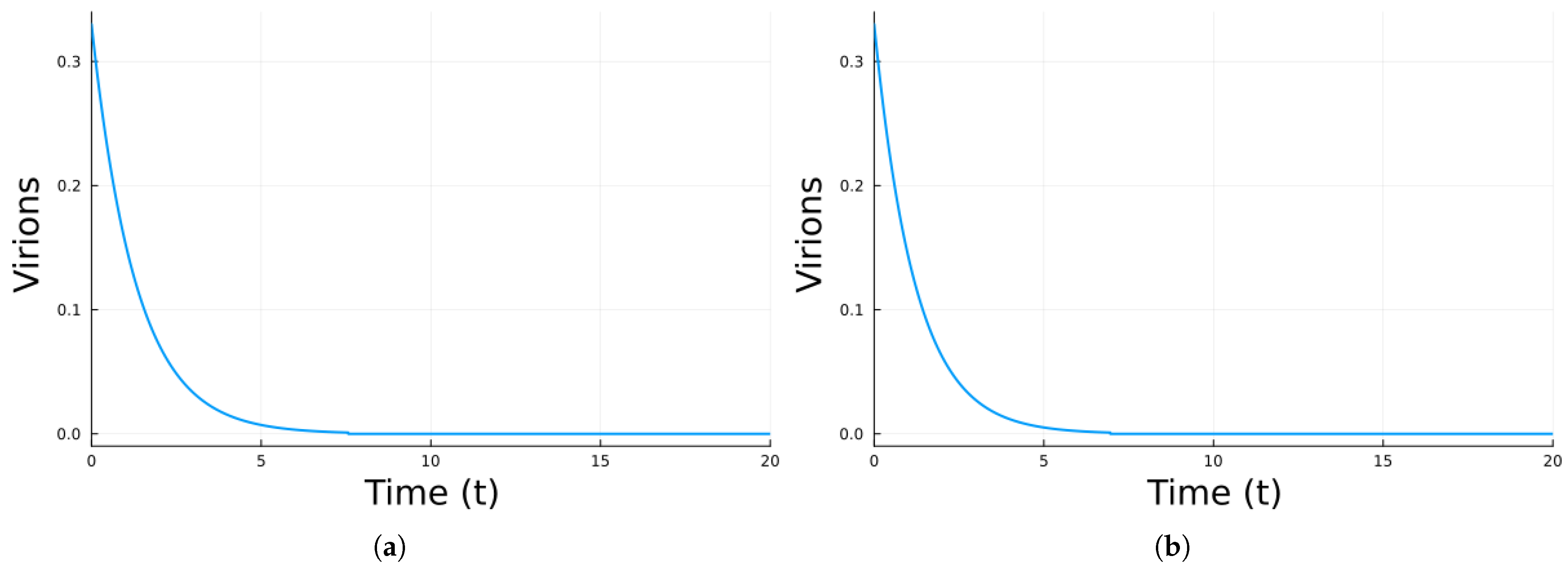
For Model 3, with the innate and adaptive immune cells and antivirals given by Equation (6), simulations were performed with two different hypotheses. In the first one, only antivirals were administered with ϵ = 0.5 , η = 0.5 and the same delays in the administration as for the previous two models. The values of the effectiveness of the antivirals to obtain a DFE are smaller than for Model 2 since there are more cells eliminating both infected cells and free virions. The infected population results are in part (a) of Figure 6. In part (b) the only treatment is vaccination. It is assumed that the vaccine adds memory to the adaptive system that is now activated to fight the virus. It is considered that there is now a natural recruitment rate of each adaptive system cell s C = 5 × 10 5 , that the production rate of antibodies, k a P , and the elimination rate of infected cells by CD8+ cells all increase by a factor of 2. Also, since the adaptive immune system has been prepared by the vaccine to the virus, the number of CD4+, CD8+ and plasma cells at the beginning of the infection is taken to be 1.0 × 10 5 , which is one order of magnitude smaller than the maximum number of these cells present during a real infection. These numbers were chosen arbitrarily to make the infection die as fast as is the case when the individual is vaccinated against the viral infection. This is, of course, a simplification of the real processes but it mimics the fact that the adaptive immune cells are better prepared to fight an infection if the individual has been vaccinated [64]. For the vaccine the infection dies faster.
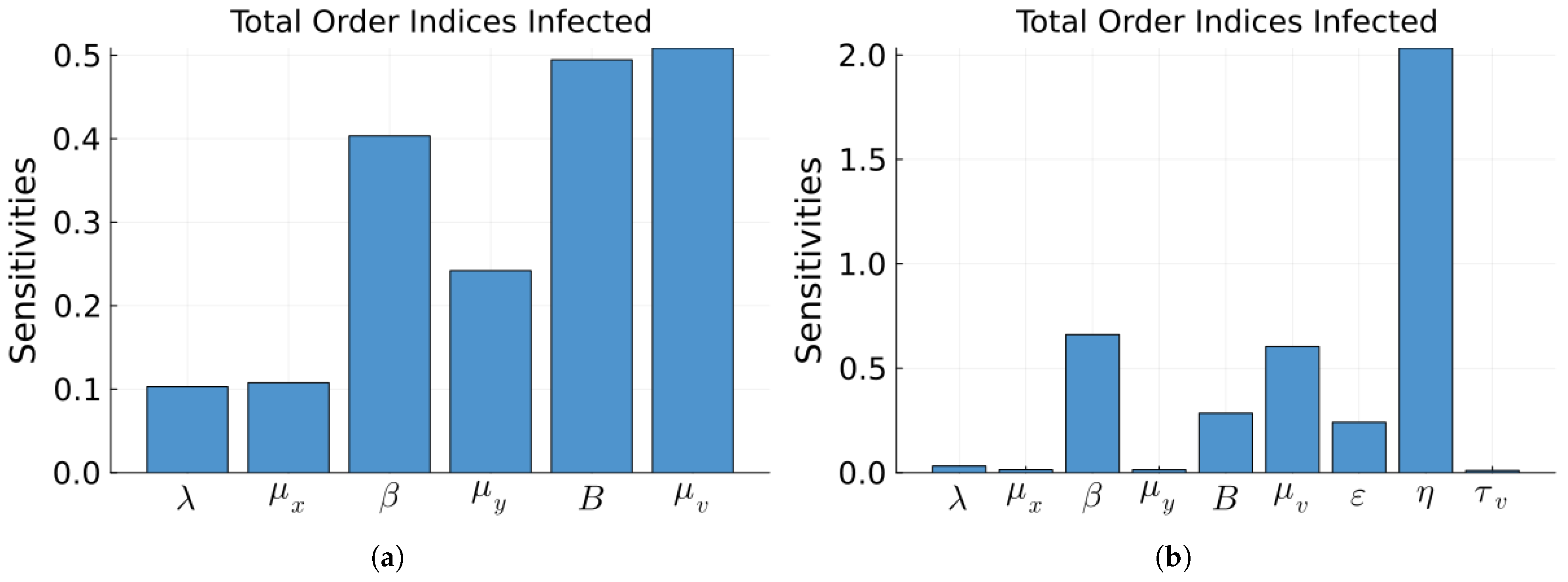
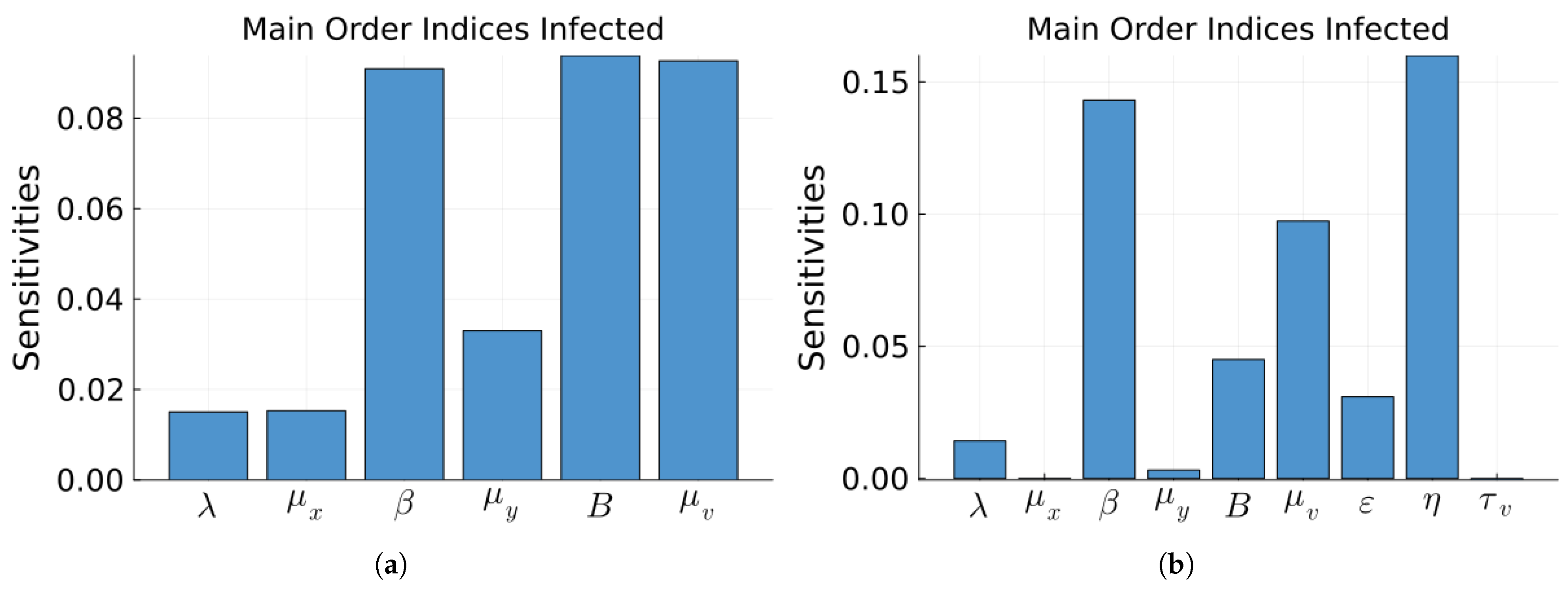
To determine the effect of changes in each parameter on the solutions of each of the models we performed a global sensitivity analysis based on Sobol indices [65]. Since the states of the models are time dependent variables, so are the sensitivity indices. The total amount of information can be reduced by taking the mean over the time of simulation, or by only considering the maximum value of the indices, or even by considering the indices of a time independent variable such as R 0 . We considered the mean. The most important states are the number of infected cells and the number of virions. We calculated the indices of both variables, but since, as expected, they are similar, we only show the indices of the infected cells. Another variance base global sensitivity method is the E-FAST [50,65]. We calculated the sensitivity indices of the infected cells given by Model 1 using both Sobol indices and E-FAST indices. Even though they give different values, the most important indices are the same. So we will only show the Sobol indices. There are two Sobol indices: main effect or first-order indices that measure the contribution to the output variance when a single parameter is varied alone while all other parameters are kept fixed, and total order indices that measure the total contribution of a parameter to the output variance, including its main effect and all interactions with other parameters. We performed the calculations using the julia software package GlobalSensitivity [66]. The range of the parameter used is the value given in Table 1 minus and plus 20%. The Sobol total order indices for the mean of the infected cells without and with antivirals, that include the interactions, are given in Figure 7. As can be seen in part (a), the most influential total order indices with no treatment are the infection index β , the number of virions from one infection B, and the death rate of the virions μ v . In part (b), the most influential total order indices with treatment are η , β , and μ v . The Sobol main order indices that do not include the interactions, for the mean of the infected cells and without and with antivirals, are given in Figure 8. As can be seen in part (a), the most influential main order indices with no treatment are still the infection index β , the number of virions from one infection B, and the death rate of the virions μ v . In part (b), the most influential main order indices with treatment are still η , β , and μ v .
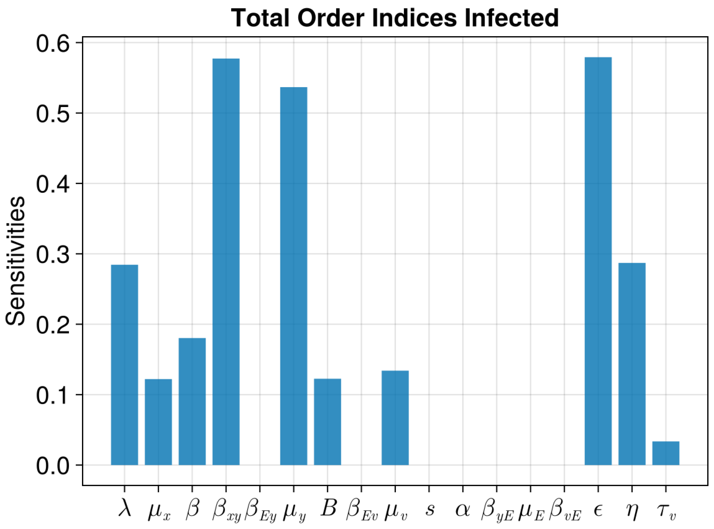
For Model 2, the Sobol total order indices of the infected cells with antivirals are shown in Figure 9. Only the results with treatment are shown. The most important indices are β x y , μ y , and η . The most influential main order Sobol indices are the same, and since we are most interested in the variations including the interactions, the plot of the main order indices is not included.
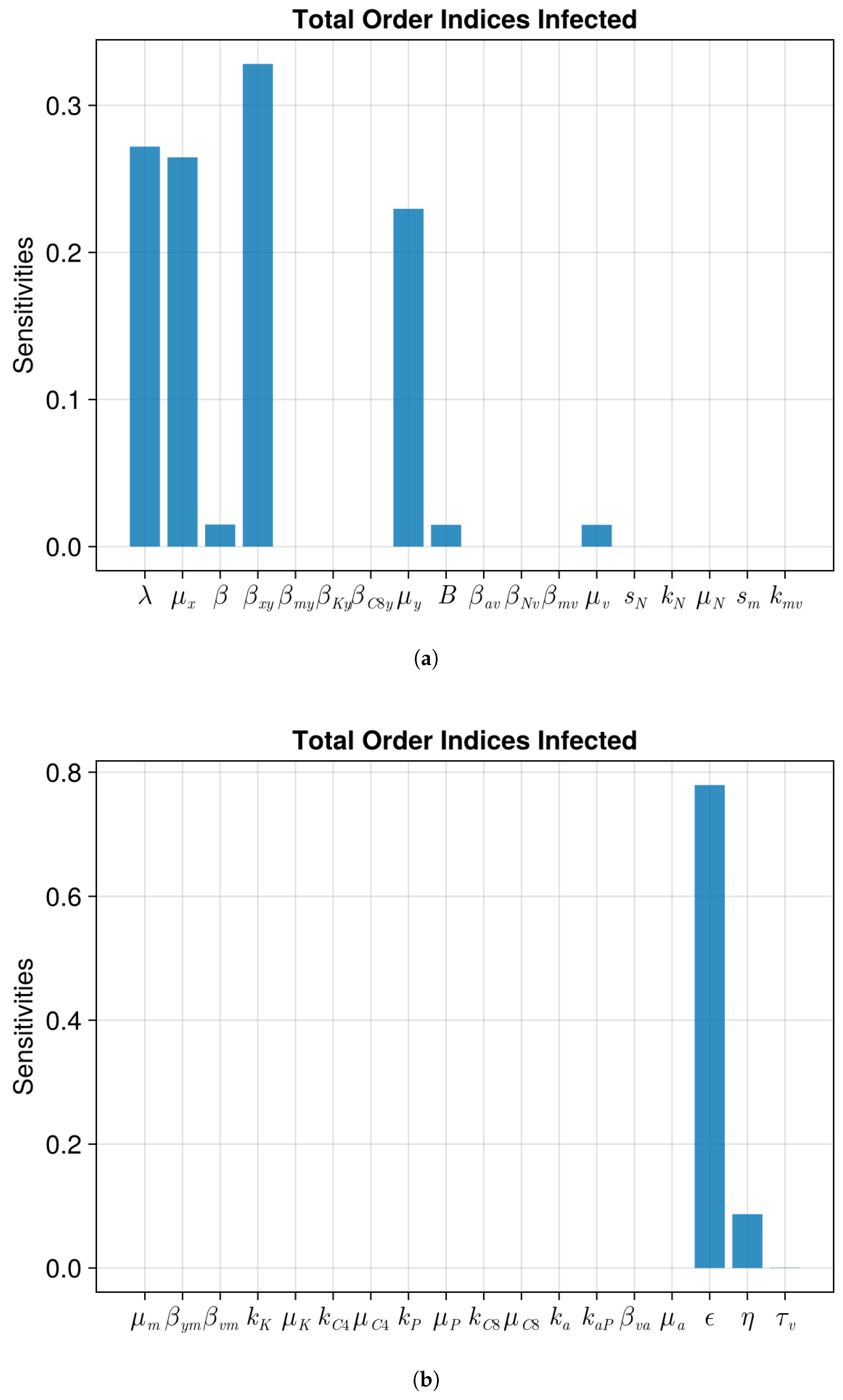
For Model 3, we present the Sobol total order indices of the infected cells, adding antivirals in Figure 10. The most relevant indices are η and β x y , with λ , μ x , and μ y next. The figure is divided in two for readability.
The most important variable is the number of infected cells. For the three models, the most influential parameters are similar.

4. Discussion

The immune system is very complex. There are many different types of cells and factors that interact among themselves, the virus, and healthy and infected cells. Including more processes makes the model more realistic, but in practice it is necessary to limit their number, both to simplify the model and better understand the most important processes. The fact that the number of parameters and data available is limited also restricts the complexity of the model. In this paper, we considered three models of increasing complexity. The simplest one includes only the effect of the immune cells eliminating the virions, with the number of immune cells implicitly taken to be constant. The second one adds one type of immune cell that eliminated both infected cells and virions. It also adds cell-to-cell infection, which is important for several viral diseases. The last model explicitly adds the most important cells of the innate and adaptive immune systems. But it only considers one chemical factor, antibodies, since they kill virions directly. The other factors and cytokines involved in signaling were assumed to have concentrations proportional to the number of cells that produce them. Also, for simplicity, we did not include some immune cells such as inactivated macrophages or dendritic cells. Model 3 includes the activation chain of the different immune cells, which makes the model more biologically realistic but mathematically more complex. We performed comparisons between three models that have different complexities. We saw that the three models have disease free and chronic equilibrium states, and found that through introducing antivirals it was possible to change the chronic equilibrium to the DFE. The antivirals were not introduced explicitly but their effect was included by modifying the infection rates and the replication factor of the virus B. We also used global sensitivity analysis to determine the parameters that cause the biggest changes in the number of infected cells. In this way, directions to better measure them can be developed. But most importantly, it can encourage research in how to change these parameters to decrease the damage from the viral infection.
All biochemical phenomena are complex and virus infections are not an exception. Mathematical models try to include all important processes but require simplifications. Some simplifications like considering deterministic processes and continuous and well-mixed populations make the mathematics more tractable. Others are performed for a lack of complete understanding of the processes and lack of data. Models with undetermined parameters are not very useful. Occam’s razor states that the model should be as simple as possible but not more simplistic. In practice, it is not trivial to decide this. The third model that we consider includes the most relevant immune cells but not all cells. It does not differentiate between activated and inactive cells. It only considers one chemical factor, antibodies, but there are several types of antibodies, and we do not differentiate among them. It also considers that the interactions are of mass action style, which is the simplest hypothesis. Even with these assumptions, it has parameters that have to be chosen while fulfilling the main criteria of making the simulations have the expected behavior. There are several ways to simplify the model [67,68]. The neutrophils and macrophages behave similarly, so they could be considered one population. The natural killer cells activate the CD4+ cells which in turn activate the plasma cells that then produce antibodies. Maybe it is possible to consider that the natural killer cells through a chain not specified produce the antibodies. Only comparisons with reliable and complete data can validate a model. But since there is still not enough experimental data, the models cannot be used to make predictions about specific virus infections. They can be used to further the understanding of the different processes involved and their relative importance. Hopefully this paper will help stimulate experimental research in within-body viruses and other parasitic infections. Then it will be possible to determine if a simpler model is enough or if even more complex models are required.

Funding

This research received no external funding.

Institutional Review Board Statement

Not applicable for studies not involving humans or animals.

Informed Consent Statement

Not applicable for studies not involving humans.

Data Availability Statement

No new data was created.

Conflicts of Interest

The author declares no conflicts of interest.

Abbreviations

The following abbreviations are used in this manuscript:
ODEOrdinary differential equation
DFEDisease free equilibrium
CEChronic equilibrium
COVID-19Coronavirus disease 2019
SARSSevere acute respiratory syndrome coronavirus 2
AIDSAcquired immunodeficiency syndrome
RNARibonucleic acid
DNADeoxyribonucleic acid
E-FASTExtended Fourier amplitude sensitivity testing

References

  1. Clark, M.A.; Douglas, M.; Choi, J. Biology 2e; Openstax: Houston, TX, USA, 2018. [Google Scholar]
  2. Taveira, N. Antivirals and Vaccines. Int. J. Mol. Sci. 2023, 24, 10315. [Google Scholar] [CrossRef]
  3. Nowak, M.A.; Bonhoeffer, S.; Hill, A.M.; Boehme, R.; Thomas, H.C.; McDade, H. Viral Dynamics in Hepatitis B Virus Infection. Proc. Natl. Acad. Sci. USA 1996, 93, 4398–4402. [Google Scholar] [CrossRef]
  4. Perelson, A.S.; Nelson, P.W. Mathematical Analysis of HIV-1 Dynamics in Vivo. SIAM Rev. 1999, 41, 3–44. [Google Scholar] [CrossRef]
  5. Baccam, P.; Beauchemin, C.; Macken, C.A.; Hayden, F.G.; Perelson, A.S. Kinetics of influenza A virus infection in humans. J. Virol. 2006, 80, 7590–7599. [Google Scholar] [CrossRef] [PubMed]
  6. Nowak, M.A.; Bangham, C.R.M. Population Dynamics of Immune Responses to Persistent Viruses. Science 1996, 272, 74–79. [Google Scholar] [CrossRef] [PubMed]
  7. Hattaf, K.; Yousfi, N. Dynamics of SARS-CoV-2 Infection Model with Two Modes of Transmission and Immune Response. Math. Biosci. Eng. 2020, 17, 5326–5340. [Google Scholar] [CrossRef]
  8. Murase, A.; Sasaki, T.; Kajiwara, T. Stability Analysis of Pathogen-Immune Interaction Dynamics. J. Math. Biol. 2005, 51, 247–267. [Google Scholar] [CrossRef] [PubMed]
  9. Kajiwara, T.; Sasaki, T. Global Stability of Pathogen-Immune Dynamics with Absorption. J. Biol. Dyn. 2010, 4, 258–269. [Google Scholar] [CrossRef]
  10. Du, S.Q.; Yuan, W. Mathematical modeling of interaction between innate and adaptive immune responses in COVID-19 and implications for viral pathogenesis. J. Med. Virol. 2020, 92, 1615–1628. [Google Scholar] [CrossRef]
  11. Bocharov, G.A.; Romanyukha, A.A. Mathematical model of antiviral immune response III. Influenza A virus infection. J. Theor. Biol. 1994, 167, 323–360. [Google Scholar] [CrossRef]
  12. Cao, P.; Wang, Z.; Yan, A.W.C.; McVernon, J.; Xu, J.; Heffernan, J.M.; Kedzierska, K.; McCaw, J.M. On the Role of CD8+ T Cells in Determining Recovery Time from Influenza Virus Infection. Front. Immunol. 2016, 7, 611. [Google Scholar] [CrossRef]
  13. Gómez, M.C.; Yang, H.M. Mathematical Model of the Immune Response to Dengue Virus. J. Appl. Math. Comput. 2020, 63, 455–478. [Google Scholar] [CrossRef]
  14. Culshaw, R.V.; Ruan, S.; Webb, G. A mathematical model of cell-to-cell spread of HIV-1 that includes a time delay. J. Math. Biol. 2003, 46, 425–444. [Google Scholar] [CrossRef] [PubMed]
  15. Pourbashash, H.; Pilyugin, S.S.; De Leenheer, P.; McCluskey, C. Global analysis of within host virus models with cell-to-cell viral transmission. Discrete Contin. Dyn. Syst. Ser. B 2014, 19, 3341–3357. [Google Scholar] [CrossRef]
  16. Shu, H.; Wang, L.; Watmough, J. Global Stability of a Nonlinear Viral Infection Model with Infinitely Distributed Intracellular Delays and CTL Immune Responses. SIAM J. Appl. Math. 2013, 73, 1280–1302. [Google Scholar] [CrossRef]
  17. Yang, Y.; Zou, L.; Ruan, S. Global Dynamics of a Delayed Within-Host Viral Infection Model with Both Virus-to-Cell and Cell-to-Cell Transmissions. Math. Biosci. 2015, 270, 183–191. [Google Scholar] [CrossRef]
  18. Zhang, S.; Li, F.; Xu, X. Dynamics and control strategy for a delayed viral infection model. J. Biol. Dyn. 2022, 16, 44–63. [Google Scholar] [CrossRef]
  19. Wang, Z.; Zhao, X.Q. A Within-Host Virus Model with Periodic Multidrug Therapy. Bull. Math. Biol. 2013, 75, 543–563. [Google Scholar] [CrossRef]
  20. Canini, L.; Perelson, A.S. Viral Kinetic Modeling: State of the Art. J. Pharmacokinet. Pharmacodyn. 2014, 41, 431–443. [Google Scholar] [CrossRef] [PubMed]
  21. Chimal-Eguia, J.C. Mathematical Model of Antiviral Immune Response against the COVID-19 Virus. Mathematics 2021, 9, 1356. [Google Scholar] [CrossRef]
  22. Xu, Z.; Song, J.; Zhang, H.; Wei, Z.; Wei, D.; Yang, G.; Demongeot, J.; Zeng, Q. A Mathematical Model Simulating the Adaptive Immune Response in Various Vaccines and Vaccination Strategies. Sci. Rep. 2024, 14, 23995. [Google Scholar] [CrossRef]
  23. Eftimie, R.; Gillard, J.J.; Cantrell, D.A. Mathematical Models for Immunology: Current State of the Art and Future Research Directions. Bull. Math. Biol. 2016, 78, 2091–2134. [Google Scholar] [CrossRef]
  24. Holling, C.S. Some characteristics of simple types of predation and parasitism1. Can. Entomol. 1959, 91, 385–398. [Google Scholar] [CrossRef]
  25. Cantrell, R.S.; Cosner, C. On the dynamics of predator–prey models with the Beddington–DeAngelis functional response. J. Math. Anal. Appl. 2001, 257, 206–222. [Google Scholar] [CrossRef]
  26. Hahl, S.K.; Kremling, A. A Comparison of Deterministic and Stochastic Modeling Approaches for Biochemical Reaction Systems: On Fixed Points, Means, and Modes. Front. Genet. 2016, 7, 157. [Google Scholar] [CrossRef]
  27. Chen-Charpentier, B. On population models with delays and dependence on past values. Axioms 2024, 13, 206. [Google Scholar] [CrossRef]
  28. Diekmann, O.; Heesterbeek, J.; Roberts, M.G. The construction of next-generation matrices for compartmental epidemic models. J. R. Soc. Interface 2010, 7, 873–885. [Google Scholar] [CrossRef]
  29. Van den Driessche, P. Reproduction numbers of infectious disease models. Infect. Dis. Model. 2017, 2, 288–303. [Google Scholar] [CrossRef] [PubMed]
  30. Hefferman, J.; Smith, R.; Wahl, L. Perspectives on the basic reproduction ratio. J. R. Soc. Interface 2005, 2, 281–293. [Google Scholar] [CrossRef] [PubMed]
  31. Murray, J.D. MathematicalBiology I. An Introduction; Springer: Berlin/Heidelberg, Germany, 2002. [Google Scholar]
  32. Allen, L. An Introduction to Mathematical Biology; Pearson-Prentice Hall: London, UK, 2007. [Google Scholar]
  33. Chen-Charpentier, B. A model of hepatitis B viral dynamics with delays. AppliedMath 2024, 4, 182–196. [Google Scholar] [CrossRef]
  34. Ciupe, S.M.; Ribeiro, R.M.; Nelson, P.W.; Dusheiko, G.; Perelson, A.S. The role of cells refractory to productive infection in acute hepatitis B viral dynamics. Proc. Natl. Acad. Sci. USA 2007, 104, 5050–5055. [Google Scholar] [CrossRef]
  35. Kim, H.Y.; Kwon, H.D.; Jang, T.S.; Lim, J.; Lee, H.S. Mathematical modeling of triphasic viral dynamics in patients with HBeAg-positive chronic hepatitis B showing response to 24-week clevudine therapy. PLoS ONE 2012, 7, e50377. [Google Scholar] [CrossRef]
  36. Herbert, J.A.; Panagiotou, S. Immune Response to Viruses. In Encyclopedia of Infection and Immunity; Elsevier: Amsterdam, The Netherlands, 2022; pp. 429–444. [Google Scholar] [CrossRef]
  37. Meischel, T.; Villalon-Letelier, F.; Saunders, P.M.; Reading, P.C.; Londrigan, S.L. Influenza A virus interactions with macrophages: Lessons from epithelial cells. Cell. Microbiol. 2020, 22, e13170. [Google Scholar] [CrossRef] [PubMed]
  38. Wang, X.L.; Wang, X.; Ho, W.Z. Roles of Macrophages in Viral Infections. Viruses 2024, 16, 1643. [Google Scholar] [CrossRef]
  39. Rouse, B.T.; Sehrawat, S. Immunity and immunopathology to viruses: What decides the outcome? Nat. Rev. Immunol. 2010, 10, 514–526. [Google Scholar] [CrossRef]
  40. Mueller, S.N.; Rouse, B.T. Immune responses to viruses. Clin. Immunol. 2009, 421–431. [Google Scholar]
  41. Gracia-Hernandez, M.; Sotomayor, E.M.; Villagra, A. Targeting Macrophages as a Therapeutic Option in Coronavirus Disease 2019. Front. Pharmacol. 2020, 11, 577571. [Google Scholar] [CrossRef] [PubMed]
  42. Chathuranga, K.; Weerawardhana, A.; Dodantenna, N.; Lee, J.S. Regulation of Antiviral Innate Immune Signaling and Viral Evasion Following Viral Genome Sensing. Exp. Mol. Med. 2021, 53, 1647–1668. [Google Scholar] [CrossRef]
  43. Rodrigo, M.B.; De Min, A.; Jorch, S.K.; Martin-Higueras, C.; Baumgart, A.K.; Goldyn, B.; Becker, S.; Garbi, N.; Lemmermann, N.A.; Kurts, C. Dual Fluorescence Reporter Mice for Ccl3 Transcription, Translation, and Intercellular Communication. J. Exp. Med. 2024, 221, e20231814. [Google Scholar] [CrossRef]
  44. Koyama, S.; Ishii, K.J.; Coban, C.; Akira, S. Innate Immune Response to Viral Infection. Cytokine 2008, 43, 336–341. [Google Scholar] [CrossRef]
  45. Ciupe, S.M.; Ribeiro, R.M.; Perelson, A.S. Antibody responses during hepatitis B viral infection. PLoS Comput. Biol. 2014, 10, e1003730. [Google Scholar] [CrossRef]
  46. Wolfram Inc. Mathematica, version 13.2; Wolfram Inc.: Champaign, IL, USA, 2022. [Google Scholar]
  47. Cleveland Clinic What Do Antivirals Treat? 2025. Available online: https://my.clevelandclinic.org/health/treatments/antivirals (accessed on 25 March 2025).
  48. Perelson, A.S. Modelling Viral and Immune System Dynamics. Nat. Rev. Immunol. 2002, 2, 28–36. [Google Scholar] [CrossRef]
  49. Ciupe, S.M. Modeling the dynamics of hepatitis B infection, immunity, and drug therapy. Immunol. Rev. 2018, 285, 38–54. [Google Scholar] [CrossRef]
  50. Marino, S.; Hogue, I.B.; Ray, C.J.; Kirschner, D.E. A Methodology For Performing Global Uncertainty And Sensitivity Analysis In Systems Biology. J. Theor. Biol. 2008, 254, 178–196. [Google Scholar] [CrossRef]
  51. Rackauckas, C.; Nie, Q. DifferentialEquations.jl—A performant and feature-rich ecosystem for solving differential equations in Julia. J. Open Res. Softw. 2017, 5, 15. [Google Scholar] [CrossRef]
  52. Press, W.H. Numerical Recipes 3rd Edition: The Art of Scientific Computing; Cambridge University Press: Cambridge, UK, 2007. [Google Scholar]
  53. Virgin, H.W.; Wherry, E.J.; Ahmed, R. Redefining Chronic Viral Infection. Cell 2009, 138, 30–50. [Google Scholar] [CrossRef] [PubMed]
  54. Wodarz, D. Mathematical models of immune effector responses to viral infections: Virus control versus the development of pathology. J. Comput. Appl. Math. 2005, 184, 301–319. [Google Scholar] [CrossRef]
  55. Kolaczkowska, E.; Kubes, P. Neutrophil Recruitment and Function in Health and Inflammation. Nat. Rev. Immunol. 2013, 13, 159–175. [Google Scholar] [CrossRef]
  56. Willenborg, S.; Eming, S.A. Macrophages–Sensors and Effectors Coordinating Skin Damage and Repair. JDDG J. Dtsch. Dermatol. Ges. 2014, 12, 214–221. [Google Scholar] [CrossRef]
  57. Nayar, S.; Dasgupta, P.; Galustian, C. Extending the Lifespan and Efficacies of Immune Cells Used in Adoptive Transfer for Cancer Immunotherapies–A Review. Oncoimmunology 2015, 4, e1002720. [Google Scholar] [CrossRef]
  58. De Boer, R.J.; Homann, D.; Perelson, A.S. Different Dynamics of CD4+ and CD8+ T Cell Responses During and After Acute Lymphocytic Choriomeningitis Virus Infection 1. J. Immunol. 2003, 171, 3928–3935. [Google Scholar] [CrossRef] [PubMed]
  59. Auner, H.W.; Beham-Schmid, C.; Dillon, N.; Sabbattini, P. The Life Span of Short-Lived Plasma Cells Is Partly Determined by a Block on Activation of Apoptotic Caspases Acting in Combination with Endoplasmic Reticulum Stress. Blood 2010, 116, 3445–3455. [Google Scholar] [CrossRef]
  60. Sagiv, J.Y.; Voels, S.; Granot, Z. Isolation and characterization of low-vs. high-density neutrophils in cancer. In The Tumor Microenvironment: Methods and Protocols; Springer: New York, NY, USA, 2016; pp. 179–193. [Google Scholar]
  61. Galli, S.J.; Borregaard, N.; Wynn, T.A. Phenotypic and Functional Plasticity of Cells of Innate Immunity: Macrophages, Mast Cells and Neutrophils. Nat. Immunol. 2011, 12, 1035–1044. [Google Scholar] [CrossRef]
  62. Derksen, L.Y.; Tesselaar, K.; Borghans, J.A.M. Memories That Last: Dynamics of Memory T Cells throughout the Body. Immunol. Rev. 2023, 316, 38–51. [Google Scholar] [CrossRef]
  63. Derksen, L.Y. Memories That Last: Dynamics of Memory Cells in Mice, Dirty Mice, and Men. Ph.D. Thesis, Utrecht University, Utrecht, The Netherlands, 2024. [Google Scholar] [CrossRef]
  64. Arunachalam, A.B. Vaccines Induce Homeostatic Immunity, Generating Several Secondary Benefits. Vaccines 2024, 12, 396. [Google Scholar] [CrossRef]
  65. Saltelli, A.; Ratto, M.; Andres, T.; Campolongo, F.; Cariboni, J.; Gatelli, D.; Saisana, M.; Tarantola, S. Global Sensitivity Analysis: The Primer; John Wiley & Sons: Hoboken, NJ, USA, 2008. [Google Scholar]
  66. Dixit, V.K.; Rackauckas, C. GlobalSensitivity. jl: Performant and Parallel Global Sensitivity Analysis with Julia. J. Open Source Softw. 2022, 7, 4561. [Google Scholar] [CrossRef]
  67. Chen, W.W.; Niepel, M.; Sorger, P.K. Classic and contemporary approaches to modeling biochemical reactions. Genes Dev. 2010, 24, 1861–1875. [Google Scholar] [CrossRef]
  68. De Boeck, J.; Rombouts, J.; Gelens, L. A modular approach for modeling the cell cycle based on functional response curves. PLoS Comput. Biol. 2021, 17, e1009008. [Google Scholar] [CrossRef] [PubMed]
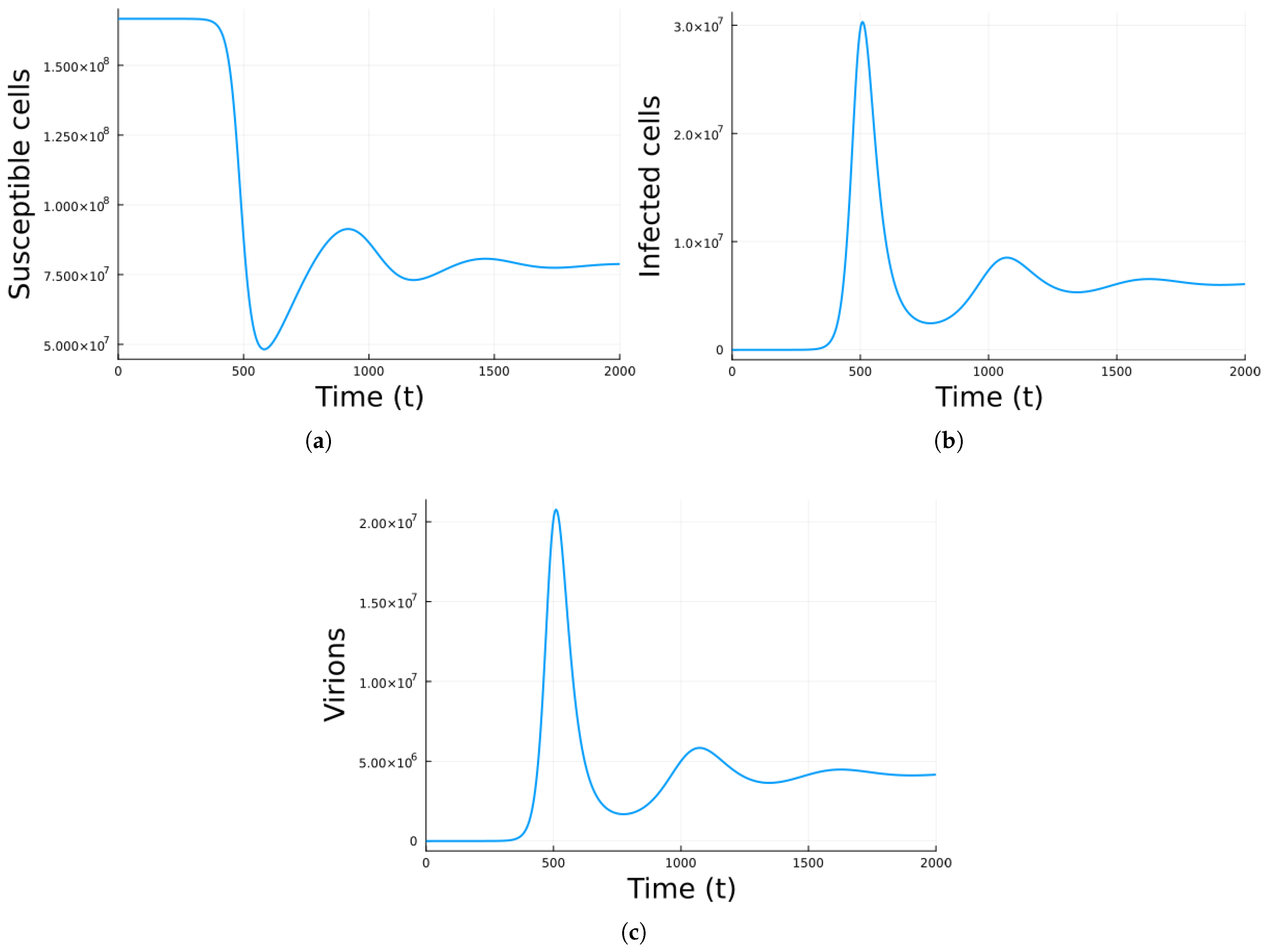
Figure 1. Simulation results for Model 1 using the parameter values in Table 1 with no antivirals. (a) Susceptible cells. (b) Infected cells. (c) Virions. The units are cells/mL for cells, virions/mL for virions, and days for time.
Algorithms 18 00544 g001
Figure 2. Simulation results for Model 2 using the parameter values in Table 2 with no antivirals. (a) Susceptible cells. (b) Infected cells. (c) Virions. (d) Effector cells. The units are cells/mL for cells, virions/mL for virions, and days for time.
Algorithms 18 00544 g002
Figure 3. Simulation results for Model 3 using the parameter values in Table 3 with no antivirals. (a) Susceptible cells. (b) Infected cells. (c) Virions. (d) Immune system cells. The units are cells/mL for cells, virions/mL for virions, and days for time.
Algorithms 18 00544 g003aAlgorithms 18 00544 g003b
Figure 4. Simulation results for Model 1 using the parameter values in Table 1 with antivirals. The plots clearly show that antivirals shown be taken as soon a possible. (a) Infected cells. (b) Virions. The units are cells/mL for cells, virions/mL for virions, and days for time.
Algorithms 18 00544 g004
Figure 5. Simulation results for Model 2 using the parameter values in Table 2. (a) Infected cells. (b) Virions. The units are cells/mL for cells, virions/mL for virions, and days for time.
Algorithms 18 00544 g005
Figure 6. Simulation results for virions using Model 3 using the parameter values in Table 3. (a) Adding antivirals only. (b) Adding vaccines only. The units are cells/mL for cells, virions/mL for virions, and days for time.
Algorithms 18 00544 g006
Figure 7. Sobol total order indices for the infected population of Model 1. (a) Without treatment. (b) With treatment. There is bar for each parameter of the model. The ranges of the parameters are the values from Table 1 +/− 20%.
Algorithms 18 00544 g007
Figure 8. Sobol main order indices for the infected population of Model 1. (a) Without treatment. (b) With treatment. The bars correspond to each of the parameters of the model. The ranges of the parameters are the values from Table 1 +/− 20%.
Algorithms 18 00544 g008
Figure 9. Sobol total order indices of the infected cells using Model 2 with treatment. The bars correspond to each of the parameters of the model. The ranges of the parameters are the values from Table 2 +/− 20%.
Algorithms 18 00544 g009
Figure 10. Sobol total order indices for Model 3 for the infected cells with antivirals. The figure is in two parts so the labels are readable. (a) are the first part of the parameters. (b) is the second part of the parameters. The bars correspond to each of the parameters of the model. The ranges of the parameters are the values from Table 2 and Table 3 +/− 20%.
Algorithms 18 00544 g010
Table 1. Parameter values for Model 1.
ParameterValueDescription
λ × 10 5 cells/mL L/drecruitment rate of susceptible cells
μ x 0.003/ddeath rate of susceptible cells
β × 10 10  mL/(virions d)infection rate of susceptible cells by virus
μ y 0.043 L/ddeath rate of infected cells
B11.16number of virions produced by 1 infected cell
μ v 0.7 L/ddeath rate of virus
Table 2. Parameter values for Model 2.
ParameterValueDescription
λ × 10 5 cells/mL L/drecruitment rate of susceptible cells
μ x 0.003/ddeath rate of susceptible cells
β × 10 10 mL/(virions d)infection rate of susceptible cells by virus
μ y 0.043/ddeath rate of infected cells
B11.16number of virions produced by 1 infected cell
μ v 0.7 L/ddeath rate of virus
β x y × 10 10 mL/(cells d)infection rate of susceptible cells by virus
β e y 0.6  × 10 3 mL/(cells d)elimination rate of infected cells by effector cells
β y e 0.6  × 10 3 mL/(cells d)removal rate of effector cells after elimination of infected cells
β e v × 10 10 mL/(cells d)elimination rate of virus by effector cells
β v e × 10 10 mL/(virions d)removal rate of y effector cells after elimination of virus
s24 cells/mL L/drecruitment rate of effector cells
α 2.2  × 10 7 /drecruitment rate of effector cells due to infected cells
μ e 0.5/ddeath rate of effector cells
Table 3. Parameter values for Model 3. Only the parameters not in Table 2 are included.
ParameterValueDescription
β m y 1.0  × 10 10 mL/(cells d)elimination rate of infected cells by macrophages
β K y 1.0  × 10 10 mL/(cells d)elimination rate of infected cells by natural killer cells
β C 8 y 2.0  × 10 8 mL/(cells d)elimination rate of infected cells by CD8+ cells
β a v 1.0  × 10 10 mL/ delimination rate of virions by antibodies
β v a 1.0  × 10 10 mL/(virions d)elimination rate of antibodies due to elimination of a virion
β N v 4.0  × 10 10 mL/(virions d)elimination rate of virions by neutrophils
β v m 4.0  × 10 10 mL/(virions d)elimination rate of virions by macrophages
s N 60.0 cells/mL L/(d virions)natural recruitment rate of neutrophils
k N 2.2  × 10 3 cells/mL L/drecruitment rate of neutrophils due to virus
μ N 3.0 cells/ ml L/ddeath rate of neutrophils
s m 0 cells/mL 1/(d virions)natural recruitment rate of macrophages
k m v 1.1  × 10 4 L/drecruitment rate of macrophages due to infected cells
μ m 4.8  × 10 2 cells/mL L/ddeath rate of macrophages
β v m 0 mL/(virions d)elimination rate of macrophages due to eliminating virions
β y m 0 mL/(cells d)elimination rate of macrophages due to eliminating infected cells
k K 2.2  × 10 3 L/dactivation rate of natural killer cells by macrophages
μ K × 10 2 L/ddeath rate of natural killer cells
k C 4 1.1  × 10 2 L/dactivation rate of CD4+ cells
μ C 4 1.1  × 10 1 L/ddeath rate of CD4+ cells
k P 1.1  × 10 2 L/dactivation rate of plasma cells
μ P 0.2 L/ddeath rate of plasma cells
k C 8 1.1  × 10 2 L/dactivation rate of CD8+ cells
μ C 8 × 10 2  L/ddeath rate of CD8+ cells
k a 3.6  × 10 3  L/mL L/dnatural recruitment rate of antibodies
k a P 2.2  × 10 2 L/(cells) L/drecruitment rate of antibodies by virus
β v a 1.0  × 10 10 mL/(virions d)elimination rate of antibodies by virus
μ a 0.3/delimination rate of antibodies
Disclaimer/Publisher’s Note: The statements, opinions and data contained in all publications are solely those of the individual author(s) and contributor(s) and not of MDPI and/or the editor(s). MDPI and/or the editor(s) disclaim responsibility for any injury to people or property resulting from any ideas, methods, instructions or products referred to in the content.