Article

A Reinforcement Learning Hyper-Heuristic with Cumulative Rewards for Dual-Peak Time-Varying Network Optimization in Heterogeneous Multi-Trip Vehicle Routing

College of Transportation Engineering, Dalian Maritime University, Dalian 116026, China
*
Author to whom correspondence should be addressed.
Algorithms 2025, 18(9), 536; https://doi.org/10.3390/a18090536
Submission received: 17 July 2025 / Revised: 20 August 2025 / Accepted: 21 August 2025 / Published: 22 August 2025

Abstract

Urban logistics face complexity due to traffic congestion, fleet heterogeneity, warehouse constraints, and driver workload balancing, especially in the Heterogeneous Multi-Trip Vehicle Routing Problem with Time Windows and Time-Varying Networks (HMTVRPTW-TVN). We develop a mixed-integer linear programming (MILP) model with dual-peak time discretization and exact linearization for heterogeneous fleet coordination. Given the NP-hard nature, we propose a Hyper-Heuristic based on Cumulative Reward Q-Learning (HHCRQL), integrating reinforcement learning with heuristic operators in a Markov Decision Process (MDP). The algorithm dynamically selects operators using a four-dimensional state space and a cumulative reward function combining timestep and fitness. Experiments show that, for small instances, HHCRQL achieves solutions within 3% of Gurobi’s optimum when customer nodes exceed 15, outperforming Large Neighborhood Search (LNS) and LNS with Simulated Annealing (LNSSA) with stable, shorter runtime. For large-scale instances, HHCRQL reduces gaps by up to 9.17% versus Iterated Local Search (ILS), 6.74% versus LNS, and 5.95% versus LNSSA, while maintaining relatively stable runtime. Real-world validation using Shanghai logistics data reduces waiting times by 35.36% and total transportation times by 24.68%, confirming HHCRQL’s effectiveness, robustness, and scalability.

1. Introduction

1.1. Background and Motivation

The rapid progress in the modern logistics industry presents both opportunities and challenges for logistics and supply chain management companies. With fluctuating customer demands, swift technological shifts, fierce competition, and the uncertainties of globalization, logistics has become increasingly challenging [1]. Brands and e-commerce retailers have significant daily inventory and return needs, imposing a substantial load on third-party transportation companies managing vehicle scheduling and task allocation. These companies must keep up with real-time inventory and return demands to make appropriate vehicle dispatches, meeting the requirements of every agent. Advances in transportation systems have enabled logistics companies to better manage their planning. The impact of service quality is enormous [2], so logistics companies need efficient delivery services and good service quality to prevent late delivery, which can lead to customer dissatisfaction and losses for the company.
To better serve their clients, supply chain management companies typically establish their own logistics platforms to facilitate transportation services. Transportation is a critical function within the supply chain, encompassing the process of delivering finished goods from distribution centers to customers. For transportation companies, effectively planning vehicle routes to deliver goods to customers while reducing the associated costs of total investment and operational expenses is a challenging issue known as the Vehicle Routing Problem (VRP) [3]. Today, the classic VRP model has been extensively studied and no longer fully meets the evolving needs of transportation, leading to the development of numerous variants that correspond to real-world issues, such as the Capacitated Vehicle Routing Problem (CVRP) [4], the Vehicle Routing Problem with Time Windows (VRPTW) [5], the Heterogeneous Fleet Vehicle Routing Problem (HVRP) [6], the Split Delivery Vehicle Routing Problem (SDVRP) [7], and the Multi-Trip Vehicle Routing Problem (MTVRP) [8], among others. Scholars have developed numerous algorithms to address the VRP and its variants. For large-scale problems, classic metaheuristic algorithms include Genetic Algorithms (GA) [9], Ant Colony Optimization (ACO) [10], Tabu Search (TS) [11], Iterated Local Search Algorithm (ILS) [12], Particle Swarm Optimization (PSO) [13], and more. For small-scale problems, precise algorithms have been proposed by, for example, Su E [14], who introduced an exact branch-and-price-and-cut algorithm to solve the pickup and delivery problem in crowd-sourced last-mile delivery (PDPCBT), and Zhou H [15], who proposed an exact branch-and-price algorithm for a two-level vehicle routing problem involving drones. The motivation for our research is a route design challenge faced by a company in Shanghai, China, aimed at fulfilling the pickup and delivery demands of each warehouse, thereby facilitating the timely distribution of goods needed by customers across the country. It is known that each warehouse is located around Shanghai, with the furthest one in Kunshan, China. For this multi-trip vehicle routing problem, we have formulated it as an NP-hard problem and incorporated significant real-world characteristics faced by the company into the model. To address this, we designed a deep learning-based hyper-heuristic algorithm and applied it to real-case scenarios to verify its effectiveness.

1.2. Related Work

The focus of this paper is a novel variant of the multi-trip vehicle routing problem, specifically the complex real-world constraints vehicle scheduling problem based on the logistics platforms of business retailers or supply chain management companies. We have considered real-world constraints such as heterogeneous fleets, time windows, warehouse loading and unloading efficiency, and peak traffic on road segments, and designed a hyper-heuristic algorithm based on reinforcement learning to address this issue. The structure of this paper is as follows: Section 2 discusses the hyperheuristic algorithm based on reinforcement learning, and proposes a hyperheuristic algorithm with cumulative reward mechanism. Section 3 defines the parameters and establishes the MILP model. Section 4 reports the relevant numerical experiments and numerical analysis. Section 5 provides conclusions and future research directions.

1.2.1. Research on Multi-Trip Vehicle Routing Problems (MTVRPs)

In this paper, we focus on the topic or keywords, restrict our search to the fields of Operations Research and Management Science, Transportation, or Traffic Science and Technology, and set the publication date between 2013 and 2024. We conducted our search on ScienceDirect and Web of Science, with the results shown in Figure 1.
From the figure, it is evident that the MTVRP has become an increasingly hot topic, and indeed, in reality, the MTVRP is more common and complex. The MTVRP was first proposed in 1990, involving a vehicle making several journeys during a day. Compared to the VRP, the MTVRP is undoubtedly more realistic, prompting more scholars to focus on this issue. Real-world problems are generally more complex than those found in academic research, making these issues more practically relevant. Pan et al. [16] studied the restocking problem faced by an automated coffee vending company for its branch locations, each with varying capacities, demands, and daytime restocking time windows, and employed a hybrid metaheuristic algorithm to address the problem. Moon et al. [17] investigated the location-routing problem with multi-compartment and multi-trip aspects and designed a corresponding hybrid genetic algorithm to solve it. Yu et al. [18] examined the Home Replenishment Delivery System (HRDS), introduced a new variant of the profitable tour problem known as the Multi-Vehicle Profitable Tour Problem with Flexible Compartments and Mandatory Customers (MVPTPFC-MC), and proposed an Adaptive Large Neighborhood Search (ALNS) algorithm to tackle this issue. You et al. [19] investigated a novel Truck Platooning Container Drayage Problem with Multiple Trips (MT-CDP-TP), developing a branch-and-price-and-cut (BPC) algorithm to solve the set partitioning model. They proposed a tailored pulse propagation algorithm based on the pricing problem of BPC. Sethanan et al. [20] introduced an integer linear programming formulation and a novel hybrid differential evolution algorithm to address the Multi-Trip Vehicle Routing Problem with backhauls and heterogeneous fleet. Neira et al. [21] presented a new compact integer programming formulation for the Multi-Trip Vehicle Routing Problem with Time Windows, highlighting the ease of implementation in any available optimization software. Liu et al. [22] proposed a dual adaptive general variable neighborhood search to tackle the Unmanned Electric Vehicle Routing and Scheduling Problem in green manufacturing systems.

1.2.2. Reinforcement Learning Approaches for MTVRP

The integration of reinforcement learning (RL) with hyper-heuristic frameworks has become an emerging trend in solving complex operational research problems. This combination leverages RL to adaptively select among multiple low-level heuristics, thereby handling large-scale instances and multiple constraints more effectively. It has been widely explored in various domains, such as heterogeneous vehicle routing problems (Qin et al. [23]), automated container terminal scheduling (Xu et al. [24]), batch flow shop scheduling (Duan et al. [25]), distributed flexible job shop scheduling (Zhang et al. [26]), and manufacturing project scheduling (Li et al. [27]), demonstrating its versatility and practical efficiency.
Building on this methodological trend, the application of RL-based hyper-heuristic algorithms to Multi-Trip Vehicle Routing Problems (MTVRPs) and related VRP variants has emerged as a promising research direction. For example, Li et al. [28] developed a novel RL-based hyper-heuristic for heterogeneous VRPs, while Zhang et al. [29] proposed a deep RL approach for heterogeneous capacitated VRPs, both demonstrating the ability of RL to manage complex vehicle constraints. Shang et al. [30] designed a Q-learning and multi-strategy hyper-heuristic for multi-compartment green routing, addressing multi-trip and multi-time-window constraints. Xu et al. [31] introduced a dynamic embedding-based RL method for VRP with multiple time windows. Other works further explore RL in combinatorial action spaces, column generation frameworks, and graph-based VRP representations (Dastpak et al. [32]). These studies illustrate that RL combined with hyper-heuristics can effectively coordinate multiple decision levels, handle complex constraints, and achieve high-quality solutions for large-scale MTVRP instances. Table 1 summarizes selected related studies.
The main contributions of this paper are summarized as follows:
  • In response to the warehouse transfer issues faced by the company’s B2C operations, we have simultaneously considered the balance of driver workload, time windows, heterogeneous fleet, loading capacity, and time-varying road networks (morning and evening peaks), which are significant real-world characteristics with substantial practical value for logistics enterprises. To date, we have not found any MTVRP studies that comprehensively account for all these realistic features.
  • To address the problem, we define this problem as the Heterogeneous Multi-Trip Vehicle Routing Problem with Time Windows and Time-Varying Networks (HMTVRPTW-TVN) and develop a mixed-integer linear programming (MILP) formulation. A dual-peak time discretization method is proposed to efficiently model time-varying networks by segmenting continuous peak periods, alongside an exact linearization technique for handling times to enable coordinated scheduling of heterogeneous fleets.
  • Based on the characteristics of this real-world problem, we propose a novel HHCRQL algorithm that incorporates reinforcement learning (RL) into MTVRP. The algorithm effectively reduces the total time required for scheduling multiple trips, with its performance advantages becoming more pronounced when handling large-scale instances.
  • We established an appropriate Markov Decision Process (MDP) model and proposed a cumulative reward assignment method based on time steps, applying the concept of cumulative rewards throughout the training process. By solving the MDP model, we effectively reduced the number of iterations and improved overall computational efficiency.

2. Materials and Methods

This section introduces the solution algorithm for the aforementioned problem. The algorithm discussed in this paper is a hyper-heuristic approach that combines Q-learning with heuristic operators (HO). The main content includes the establishment of an MDP model, the definition of specific state sets, action sets, and so on.

2.1. Heuristic Operators–Reinforcement Learning Framework

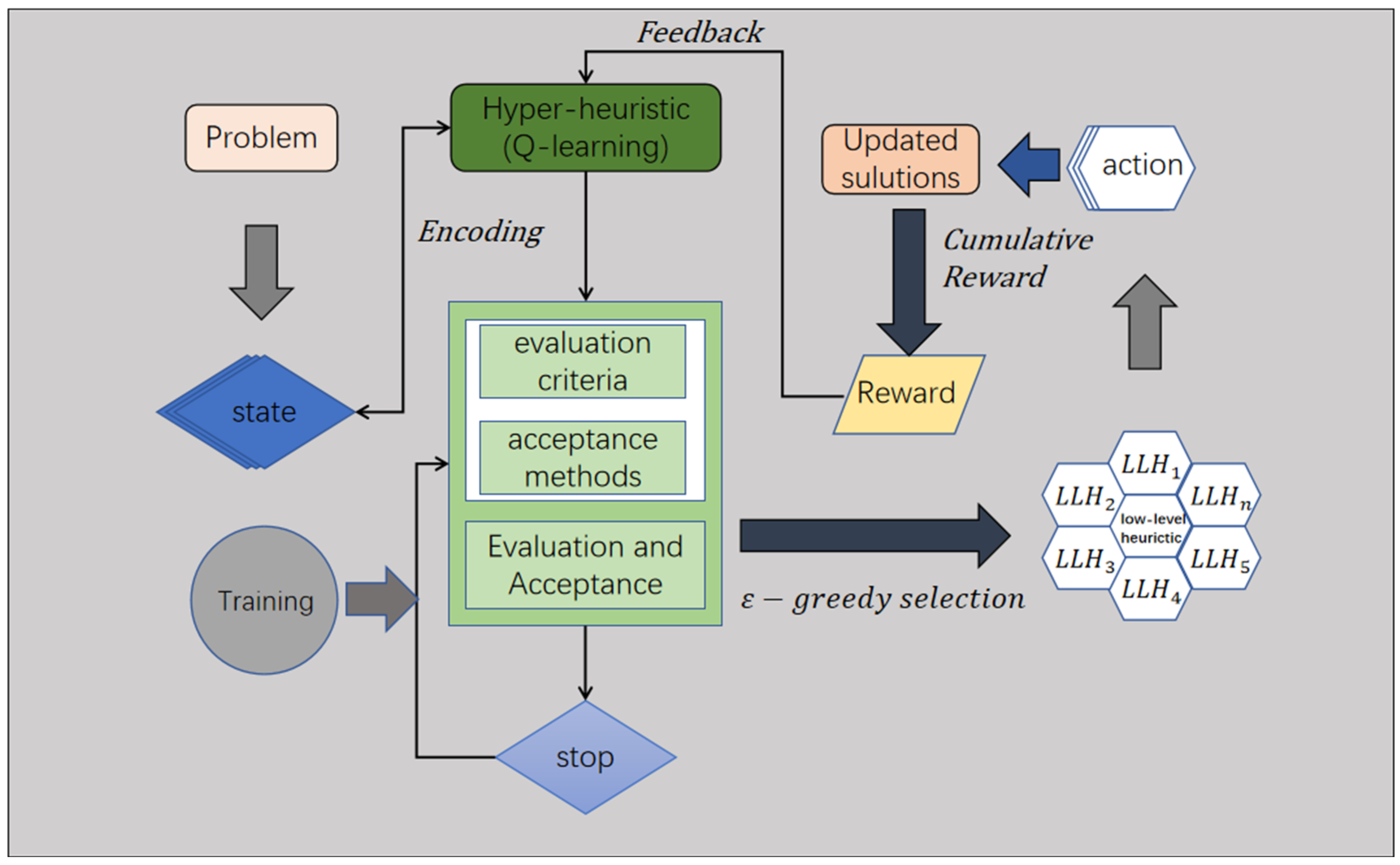
Due to the combinatorial optimization nature of the logistics platform’s multi-reality constraint scheduling problem, it is challenging to enumerate all solutions through exhaustive methods. Therefore, optimization algorithms require high computational efficiency, and hyper-heuristic algorithms are well suited for this scenario. A typical hyper-heuristic (HH) structure includes two levels: low-level heuristics (LLHs) and high-level heuristics (HLHs) [44]. Low-level heuristics encompass solution representation, computation functions, and a set of LLHs, which are specific problem operators directly applied to solutions, also known as heuristic operators (HOs). High-level heuristics are responsible for two main tasks: selecting HOs to generate new solutions and evaluating their acceptability. Both significantly impact the performance of the hyper-heuristic model, making the development of advanced and low-level strategies for specific problems a significant challenge. To address this challenge, we have developed a reinforcement learning-based hyper-heuristic (HO-RL) that leverages the strengths of different HOs. The RL method is a high-level strategy that chooses the appropriate LLH based on the environment. Specifically, the HO-RL framework starts with an initial solution and then iteratively improves it using HOs. At each iteration, RL first invokes a selection mechanism to choose the most suitable HO based on performance metrics. Then, it applies the HO to the current solution and generates a new solution. Finally, RL invokes acceptance criteria to determine whether to accept the new solution. The goal is to automatically select effective HOs at each decision point, as illustrated in Figure 2.
The process of selecting a heuristic operator (HO) can be viewed as a Markov Decision Process (MDP), where the agent must choose from a set of actions in a set of states with unknown reward models. Q-learning is a model-free reinforcement learning algorithm that learns to maximize cumulative rewards by learning a policy. In Q-learning, the agent learns an action–value function (Q-function) through interaction with the environment, which estimates the expected utility of taking a specific action in a given state. The core of Q-learning is the trade-off between exploration and exploitation. In the following sections, we introduce the construction of the specific MDP model, including the definition of state sets, action sets, selection strategies, and the reward function.

2.1.1. Initial Solution Generation

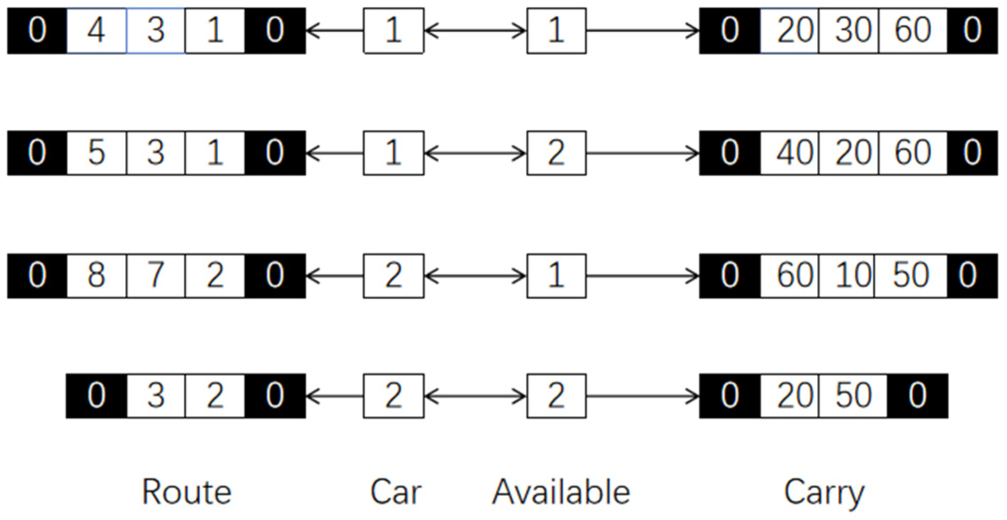
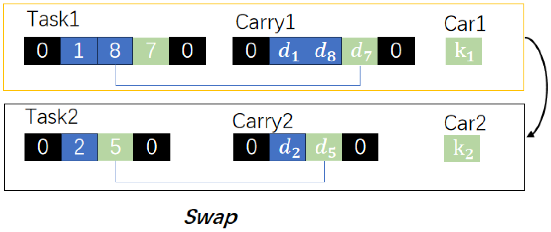
This paper begins by employing a greedy algorithm to obtain an initial near-optimal solution. This initial solution serves to narrow the solution space and reduce the algorithm’s overall running time. The solution is structured by separating the number of vehicle uses (available), vehicle sequence number (car), operating routes (task), and cargo quantity (carry) into distinct lists. These four lists collectively define the initial solution state. A key advantage of this representation is its facilitation of heuristic operator application. A critical design decision within the HO-RL framework involves the representation of solutions in the search space. To clarify this representation, a simple numerical illustration is provided. Figure 3 depicts a candidate solution involving 5 warehouses and 2 vehicles, each assigned between 3 and 5 tasks. The left side shows the four vehicle routes, the center displays the associated vehicles and their available times, and the right side indicates the loading quantity.

2.1.2. Low-Level Heuristic Operator Operations

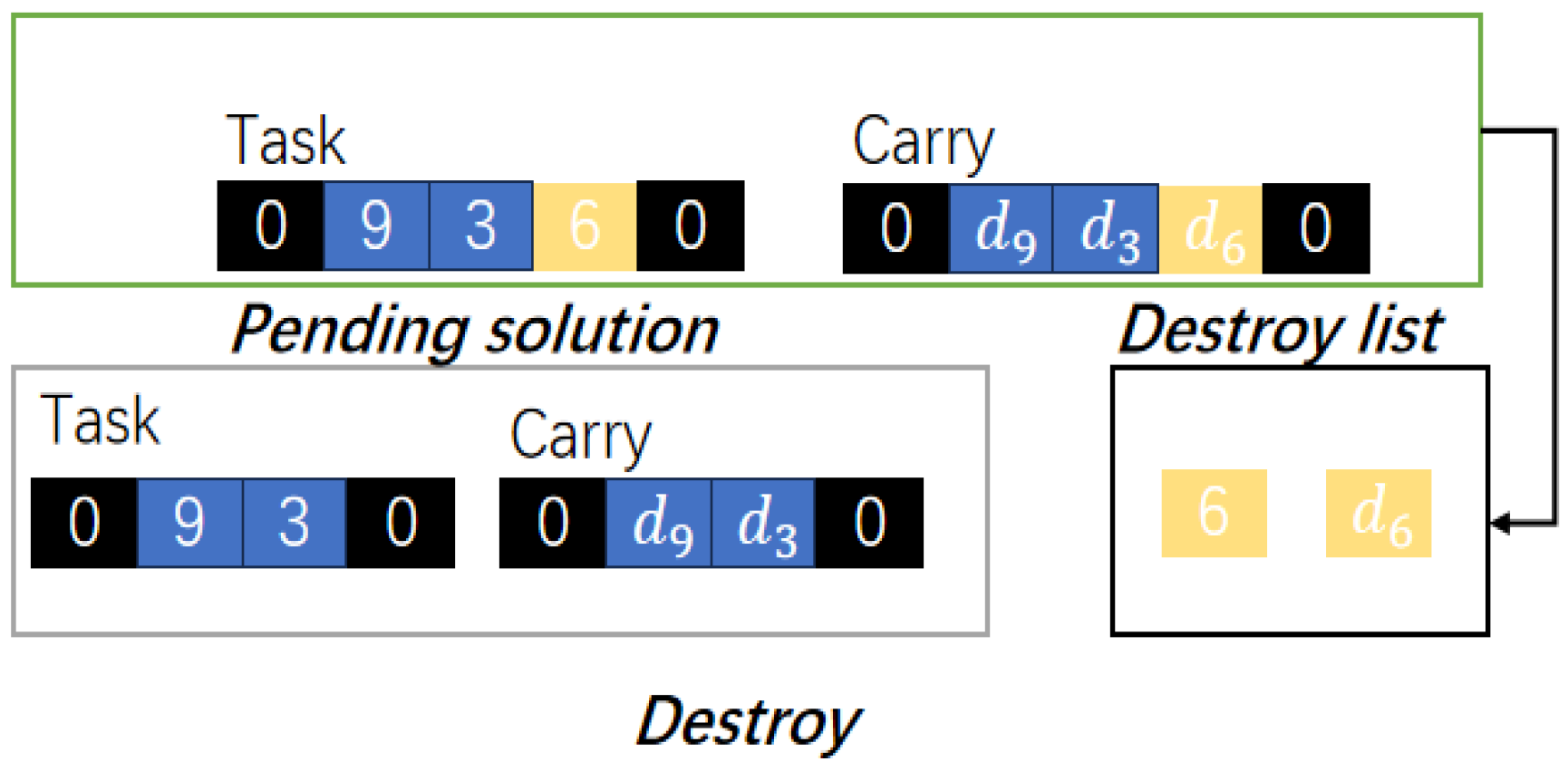
For the generated initial solution, we design and apply a set of heuristic operators—destruction, repair, and exchange—to iteratively improve the routing solution. In the destruction phase, as shown in Figure 4, two strategies are used to increase solution diversity and enable local search: maximum saving node removal, which deletes the node that yields the largest time saving to break high-efficiency segments, and longest route removal, which removes the route with the longest travel time and releases the corresponding vehicle, allowing tasks to be reassigned.
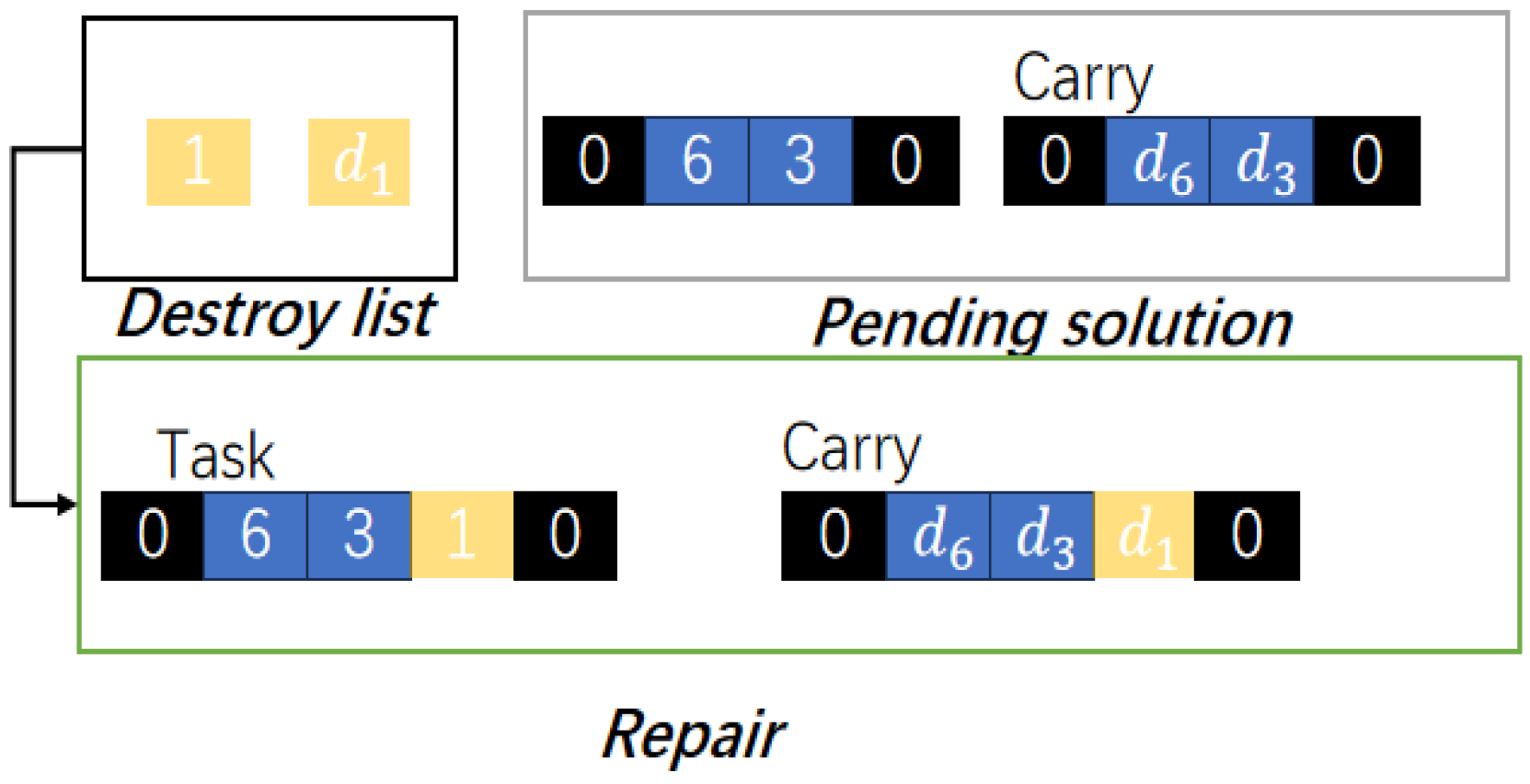
In the repair phase, as shown in Figure 5, removed nodes from the destroy_list are reinserted using greedy insertion or random insertion. Greedy insertion tries all feasible positions and selects the one with minimal incremental travel cost while respecting vehicle capacity. Random insertion selects feasible routes and positions randomly; if a node cannot be inserted into any existing route, a new route is created using an available vehicle. Both strategies ensure all removed customer demands are reinserted, balancing cost optimization and stochasticity.
In the exchange phase, as shown in Figure 6, two types of swaps are applied to improve route quality: intra-route customer exchange optimizes local visiting sequences, and inter-route customer exchange swaps customer nodes between routes under capacity constraints to balance workloads and reduce total travel time. Additionally, a vehicle workload balancing step swaps entire routes between vehicles to reduce variance in route durations and enhance resource utilization. By iteratively applying these destruction, repair, and exchange operators, the method effectively explores the solution space, maintains feasibility, optimizes total travel cost, and improves vehicle utilization.

2.2. MDP Model Establishment

Q-learning is one of the most effective value-based reinforcement learning (RL) algorithms, with the goal of estimating the Q-values of the optimal policy. The construction of a Markov Decision Process (MDP) is considered one of the most critical steps in Q-learning. An MDP can typically be described by four elements: the state set, the action set A, the reward function, and the policy function. The Q-table is updated based on a comprehensive consideration of the experienced states, selected actions, and the rewards obtained by the agent. The Q-values, which characterize the rationality of action selection, are calculated based on a comprehensive consideration of the experienced states, selected actions, and the rewards obtained by the agent. The Q-value update function is performed by the following formula:
Q s t , a t Q s t , a t + α r t + γ m a x Q s t + 1 , a t + 1 Q s t , a t

2.2.1. Definition of the State Set

To effectively represent the decision-making process in the Heterogeneous Multi-Trip Vehicle Routing Problem with Time Windows and Time-Varying Networks (HMTVRPTW-TVN), this study designs the state space within the framework of a Markov Decision Process (MDP), as shown in Table 2. The design objective is to extract a limited number of features that capture the key characteristics of the dispatching environment, ensuring both theoretical soundness and learning efficiency, while maintaining sufficient expressive power and operational relevance. In traditional reinforcement learning, state space design faces the dual challenge that excessively large or irrelevant state dimensions can cause the “curse of dimensionality” and sample sparsity, while overly simplified states may omit critical decision information and reduce the effectiveness of policy learning.
Accordingly, the state is defined as a 4-tuple:
s = ( F , V , T r , U )
composed of four discretized dimensions:
(1)
Feasibility Indicator: F
Feasibility is a fundamental constraint in vehicle routing, directly influencing action selection and search direction. A binary variable F is used to indicate whether the current solution satisfies all constraints, where F = 1 denotes feasibility and F = 0 denotes infeasibility. This enables the policy to quickly identify and prioritize feasible regions of the solution space.
(2)
Number of Vehicle Types: V
This is the count of distinct vehicle types currently used in the solution. V quantifies fleet heterogeneity and problem complexity: higher V typically implies more complex assignment and compatibility considerations. Using a vehicle-type count as a state component enables the policy to adapt to different fleet compositions; when necessary, VVV can be coarsely discretized (e.g., V = 1, V = 2–3, V ≥ 4) to control state-space growth.
(3)
Remaining Task Ratio Segmentation: T r
The remaining demand ratio—defined as the fraction of unserved demand relative to initial demand—is discretized into a small number of intervals to represent progress stages of the routing problem. In this study, we use four intervals: [0, 0.25), (0.25, 0.5], (0.5, 0.75], and [0.75, 1.0]. T r captures the search horizon and priority structure for remaining tasks while limiting state cardinality.
(4)
Vehicle Load Utilization Interval: U
The overall fleet load utilization (aggregate load/aggregate capacity) is discretized into three intervals: low (<33%), medium (33–66%), and high (>66%). U encodes resource utilization efficiency and helps the policy distinguish between states that require load consolidation, redistribution, or capacity increase.
Each chosen state component is explicitly tied to core constraints or optimization objectives of HMTVRPTW-TVN, thereby ensuring that the state space is both informative and compact. Discretization balances representational fidelity and computational tractability, mitigating exponential growth in the number of states and improving training efficiency and convergence stability for tabular Q-learning. Finally, through construction, the state set is intended to satisfy the Markov property in the sense that it contains the information necessary for immediate decision-making; state transitions are then modeled as dependent only on the current state and the selected action, consistent with MDP theory.

2.2.2. Design of Action Set and Reward Function

In a Markov Decision Process (MDP), the action set is a core component, representing all possible actions an agent can take in a particular state. The design and selection of the action set directly affect the agent’s learning efficiency and the quality of final decision-making. For each state, the action set may be fixed or may vary depending on the state. It can be defined as follows:
A s = a 1 , a 2 , a 3 , , a n
In the context of the Markov Decision Process (MDP), a i represents the i -th action selected in state s . In this paper, the action set is set to different heuristic operators, as shown in Table 3. During each iteration, the agent will select different heuristic operators to obtain corresponding rewards, with the reward design aimed at accelerating the search process and achieving optimization goals. As shown in Table 3, when an action a n is chosen from the a c t i o n   s e t , the agent will execute the corresponding heuristic operators. Secondly, a reward function with crossover probability should be designed to assess whether the value of the chosen action is reasonable; under the same algorithm, different reward functions may yield different results. The setting of the reward function determines the convergence speed and efficiency of the algorithm. The reward function in this paper is defined by the following equation:
R action = 1 , Fit best solution i t + 1 Fit best solution i t 0 1 , Fit best solution i t + 1 Fit best solution i t > 0
The reward function R a c t i o n represents the reward obtained for taking action a in states. F i t b e s t ( s o l u t i o n i t + 1 ) denotes the best fitness value of the i-th solution in the t + 1-th episode, F i t b e s t s o l u t i o n i t denotes the best fitness value of the i-th solution in the t-th episode. When the best fitness value of the i -th solution in the (t + 1)-th episode is greater than that in the t-th episode, the reward is a positive value. Conversely, the reward will become positive with probability p and remain negative with probability 1 p . The distinction between positive and negative values is that actions corresponding to positive rewards will increase in frequency, while those corresponding to negative rewards will decrease. This involves the policy function π , which we will introduce in the next section.

2.2.3. Policy Function

In this paper, the ε - g r e e d y policy is chosen as the action selection strategy. The ε - g r e e d y policy is a method that balances exploration and exploitation. Specifically, it selects the current optimal action with a probability of 1 ε and selects an action randomly with a probability of ε . In this paper, the ε - g r e e d y policy can be represented by the following equation. ε represents the exploration rate, | A | represents the size of the action set, Q s , a denotes the Q-value of taking action a in state s , and a represents the optimal action in state s , that is, a = a r g m a x a a c t i o n s Q s , a . We use the indicator function I ( x ) to represent whether certain conditions are met.
P s , a = 1 ε I a = a + ε 1 A a A I a = a

2.3. Hyper-Heuristic Based on CR-Q-Learning

This section delves into the hyper-heuristic based on CR-Q-learning (HHCRQL). We start by outlining the core components of the high-level heuristic (HLH), specifically the CR-selection strategy. Then, we describe the main logical flow of the CR-Q-learning process.

2.3.1. CR-Selection Strategy

We introduce a cumulative-reward credit-assignment mechanism that jointly accounts for the feasibility and quality of the current solution, while employing an ε-greedy strategy to select heuristic operators (HOs). Although ε-greedy is effective for low-level heuristic (LLH) selection, its credit-allocation rule remains simplistic. Cumulative rewards evaluate HO efficacy comprehensively through two performance indicators—applicability and feasibility—thereby not only identifying superior HOs but also intermittently admitting alternative HOs to sustain population diversity. Integrating ε-greedy with cumulative-reward credit allocation naturally balances the production of high-quality individuals with the preservation of population diversity. This cumulative philosophy is realized via a two-phase reward-function update: immediately after an LLH operation and again when determining whether the updated individual outperforms its predecessor. These updates accumulate, progressively refining action selection and contracting the solution space.

2.3.2. HHCRQL Algorithm Procedure

The design and selection of heuristic operators are crucial to the performance of the algorithm. Effective heuristic operators can significantly enhance the efficiency and quality of solutions. Many heuristic algorithm designs involve a variety of operators, such as swap, mutation, destruction, merge, and shake operators. The role of the swap operator, for example, is to exchange nodes in a route or variables that need to be swapped. Heuristic algorithms typically fix the sequence of several operators, starting from an initial solution and continuously operating until certain conditions are met. The advantage of reinforcement learning is its ability to learn and dynamically adjust the order of operators for optimal results. Through Q-learning, initial states are selected randomly, different actions are taken, and each action yields a corresponding reward. At this point, the time step ends, and the updated Q-table is fed back to the agent. This Q-table plays a role in feedback and learning for the next time step. The agent will dynamically learn and adjust based on the rewards corresponding to actions in the Q-table for the next time step. If the reward is positive, the selection of actions by the corresponding heuristic operators will be strengthened; if negative, it will be weakened accordingly. Continuously obtaining states, executing actions with high rewards, updating the Q-table, and dynamically adjusting constitute the process of reinforcement learning. The pseudocode for the HHCRQL is shown below (Algorithm 1).
Algorithm 1 HHCRQL
HHCRQL Algorithm parameters: number_episodes (max_e), max_step (max_s), episode (e), step (s), Q table, state set (S), action set (A), learning rate (alpha), exploration rate (epsilon), discount factor (gamma).
1. Initial solution generation
2. Initialize the Q table
3. Input: algorithm parameters to HHCRQL Algorithm
4. while episode (e) < max_e do
5. s i : choose state (F, V, T r , U)
6. for time step (t) in max_step (max_s)
7. a i choose action according to ε-greedy
8. Execution: executes the selected action a i based on the s i
9. F f e : Determination of the feasibility of the current time step
10. if feasibly:
11. r e : calculate the reward
12. F v e : Fitness value calculation of the current time step
13. if better F v e
14. r e : accrue reward and update Q table
15. else: no accrue reward
16. else: give punishment in reward and update Q table
17. t = t + 1
18. END While: satisfy stopping criterion
19. Output: optimal solution and Q table

3. Problem Description and Modeling

In this section, we specifically analyze the concrete elements of this real-world problem and position it as the Heterogeneous Multi-Trip Vehicle Routing Problem with Time Windows and Time-Varying Network (HMTVRPTW-TVN). We have analyzed and established a corresponding mixed-integer linear programming (MILP) model that can be adapted for solution by any commercial solver.

3.1. Problem Description

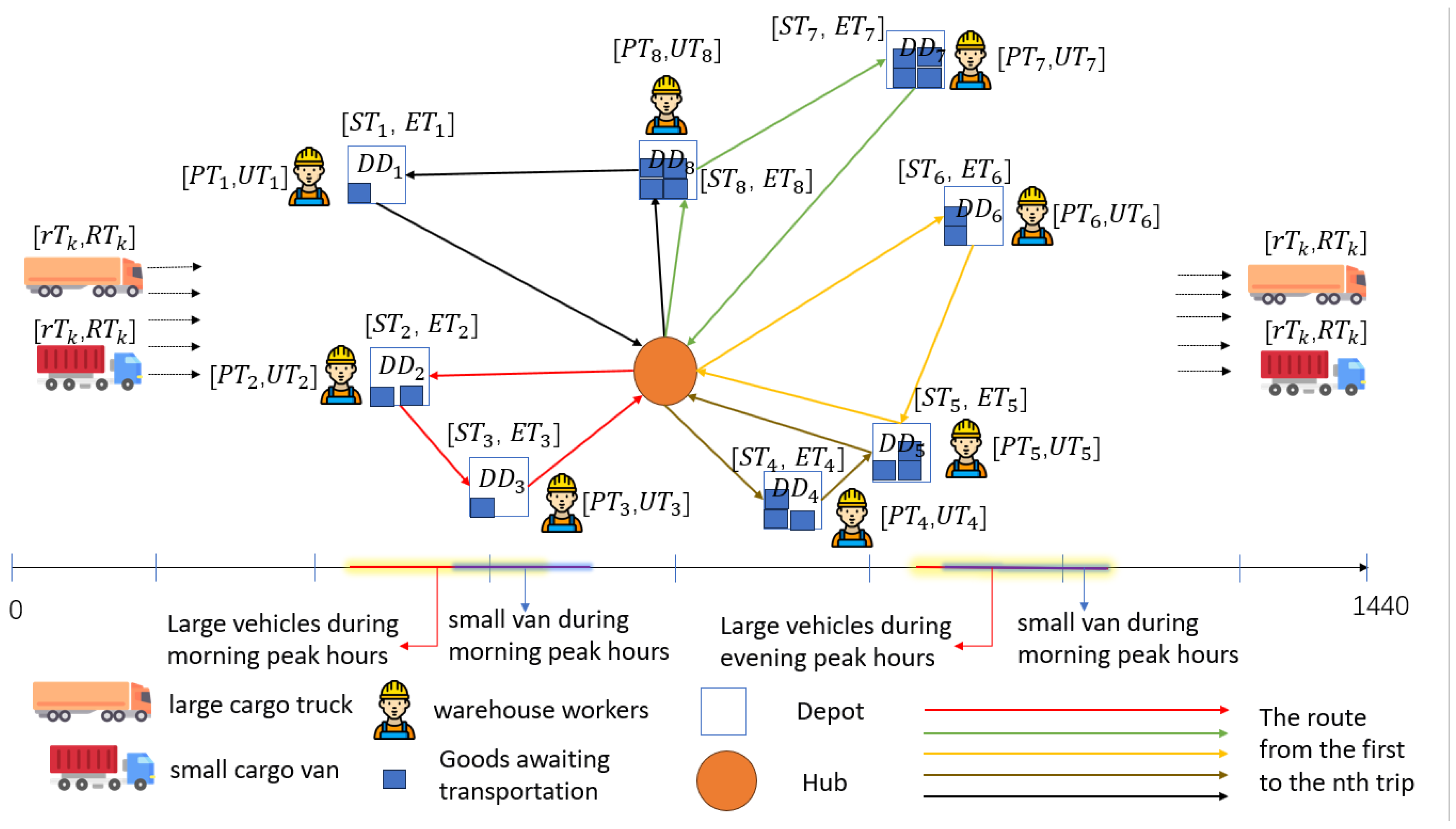
The vehicle dispatch system receives reports from various outlets (warehouses) every day at dawn, detailing the pickup and delivery volumes for the day. Dispatchers arrange drivers to depart from the distribution center, known as the super-hub, to execute transportation tasks. To fulfill the daily transportation tasks, the company has established a fleet for cargo transportation. The tasks vary daily, and at times, it is necessary to engage crowd-sourced vehicles to assist with transportation duties. Due to the fleet’s characteristics, there are different models of vehicles and various types of drivers. One type is directly employed by the company, and the other is outsourced. When assigning tasks, efforts are made to balance the workload of drivers. The locations of the warehouses are fixed, and their working time windows are also set, so the vehicle dispatch system schedules and routes the heterogeneous fleet for multiple departures at appropriate times(as shown in Figure 7): departing from the super-hub’s parking lot, executing a series of transportation tasks according to the dispatch orders, and returning to the super-hub parking lot. The challenge lies in determining the right time to depart, avoiding morning and evening peak traffic while arriving within the working time window of the warehouses to load and unload. Therefore, this problem can be formally defined as an optimization problem, known as the Heterogeneous Multi-Trip Vehicle Routing Problem with Time Windows and Time-Varying Network (HMTVRPTW-TVN). In a directed network G = ( V , E ) , where V is the set of nodes, including a distribution center D and a set of pickup warehouses C , and E is the set of arcs, corresponding to the connections between nodes. For each arc ( i , j ) E , there is an associated travel time t i j . Each warehouse C E has a working window [ S T i , E T i ] and a break window [ P T i , U T i ] . Each vehicle’s driver is fixed, and the driver’s working time window is [ r T i , R T i ] .

3.2. Parameter and Variable Definitions

We define the notation and variables for HMTVRPTW-TVN. Table 4 lists the modeling variables, and Table 5 lists all notations along with the relevant parameters used.

3.3. Construction of HMTVRPTW-TVN

Since the information (vehicle information, warehouse information, pending pickup information, working time window information, etc.) is updated through daily morning reports, this information can be considered as known. The HMTVRPTW-TW problem formulation is as follows:
  • Objective function consisting of two components, with cost calculation varying by vehicle type:
    M i n i m i z e   z =   o b j l a r g e + o b j s m a l l
    obj_large = i V j V k K q Q t i , j o r i g x i , j k , q + F T j x i , j k , q + x i , j k , q d j k , q / e j + w j k , q
    obj_small = i V j V k K q Q [ t i , j a c t u l x i , j k , q + F T j x i , j k , q + x i , j k , q d j k , q / e j + w j k , q ]
    Subject to the following:
  • Capacity and demand constraints:
    j c d j k , q Z k , q c k       k K ,       q Q
    k K q q i V x i , j k , q   d j k , q + M Z k , q 1 D D j       j C    
    T L k q = j c d j k , q       k K ,     q Q
    d D e k , q = T L k q       k K ,     q Q
  • Flow conservation constraints:
    j V x D s , j k , q = i V x i , D e k , q = Z k q     k K ,       q Q  
    j V x j , D s k , q = J V x D e , j k , q = 0       k K ,       q Q  
    j V x i , j k , q = j V x j , i k , q     k K , i V       q Q
  • Vehicle task execution sequence constraints:
    S j k , q   S i k , q + w i k , q + F T i + δ i / e i   + t i , j k , q M 1 x i , j k , q   i V , j V , k K , q Q
    δ i = T L k q   , i f     i = 0   d i k , q ,   o t h e r s i V , j V , k K , q Q
    t i , j k , q = t i , j o r i g   ,     k K l   t i , j , k , q a c t u a l ,     k K s i V , j V , k K , q Q
  • Peak period constraints for small vehicles:
    D T i k , q = S i k , q + w i k , q + F T i + δ i / e i      
    D T i k , q   L T m M ( 1 y i , j , k , q 1 )             i V , j V , k K , q Q
    D T i k , q   L T n + M ( 1 y i , j , k , q 1 )               i V , j V , k K , q Q
    D T i k , q   T P m M ( 1 y i , j , k , q 2 )               i V , j V , k K , q Q
    D T i k , q   T P n + M ( 1 y i , j , k , q 2 )                 i V , j V , k K , q Q
    t i , j , k , q a c t u a l = t i , j s m a l l ( y i , j , k , q 1 + y i , j , k , q 2 ) + t i , j o r i g ( 1 y i , j , k , q 1 y i , j , k , q 2 )       i V , j V , k K , q Q
    z i , j , k , q = t i , j , k , q a c t u a l x i , j k , q     i V , j V , k K , q Q
  • Peak period constraints for large vehicles:
    D T i k , q   L T γ + M ( 1 a i , j , k , q 1 )     i V , j V , k K , q Q
    D T i k , q   L T δ M ( 1 a i , j , k , q 2 )     i V , j V , k K , q Q
    a i , j , k , q 1 + a i , j , k , q 2 x i , j k , q     i V , j V , k K , q Q
    t i , j a r r = D T i k , q + t i , j o r i g     i V , j V , k K , q Q
    t i , j a r r T P γ + M ( 1 a i , j , k , q 3 )     i V , j V , k K , q Q
    t i , j a r r T P δ + M ( 1 a i , j , k , q 4 )     i V , j V , k K , q Q
    a i , j , k , q 1 + a i , j , k , q 2 x i , j k , q     i V , j V , k K , q Q
  • Warehouse worker rest time-window constraints:
    S j k , q + w j k , q   P T i M ( 1 a j k , q )             j C , k K , q Q
    S j k , q + w j k , q U T j + M ( 1 b j k , q )       j C , k K , q Q
    a j k , q + b j k , q 1     j C , k K , q Q  
  • Driver working time-window constraints:
    r T k   S D s k , q R T k             k K , q Q
  • Trip count limitations:
    q Q Z k , q | Q |       k K
  • Trip sequence limitations:
    Z k , q Z k , q 1       k K ,       q 1  
  • Warehouse operating time-window constraints:
    S T k   S i k , q E T k             k K ,   j C , q Q
  • Other constraints (non-zero loading, inter-trip time coupling, and binary variable declarations):
    d j k , q   M i V x i , j k , q           k K , j C , q Q
    S D e k , q + w D e k , q + F T D e + d D e k , q / e D e S D s k , q + 1 + M ( 1 Z k , q )   k K , q < | Q | 1  
    x i , j k , q = 0 :   others 1 : if   vehicle   k   travels   along   arc   ( i , j )   during   its   q th   trip
    Z k , q = 0 :   others 1 : if   vehicle   k   makes   the   q th   trip

4. Numerical Experiments

In this section, we conduct numerical experiments using the R-series data from the Solomon instances to validate the applicability of the proposed algorithm. Comparative experiments are carried out, where the results are compared with those obtained by other algorithms or commercial solvers to verify the effectiveness of both the model and the algorithm. Finally, the HHCRQL algorithm is applied to solve problems of varying scales, and the results are compared with these methods to demonstrate the practicality and high performance of the algorithm.

4.1. Solution Results Based on Real Cases

4.1.1. Real-Case Analysis

This section conducts numerical experiments using real data from a distribution center of a Shanghai-based supply chain company to evaluate the performance of the HHCRQL algorithm. For convenience in the experiments, the distribution center is labeled as sup-hub 0, and the warehouses are numbered from 1 to 13. Detailed data for each warehouse are provided in Appendix A.
Loading at the warehouses is conducted in pallets, with the loading rate measured in cubic meters per minute. Vehicles are numbered from 1 to 12, with vehicles 1–4 being large vehicles measuring 17.5 m in length and having driver working time windows of [330–1500]. Vehicles 5–12 are smaller, measuring 9.6 m in length, with driver working time windows of [360–1410].

4.1.2. Real-Case Study and Result Analysis

To comprehensively evaluate the model and algorithm, this study further compares them with the company’s actual scheduling plans. Using total time, warehouse waiting time, and vehicle utilization as evaluation metrics, Table 6 shows that the solutions obtained by our algorithm outperform the company’s actual dispatch center in both total time cost and warehouse waiting time. Furthermore, due to a more balanced workload distribution, more vehicles are utilized, allowing large vehicles to complete their tasks and finish shifts earlier, thereby avoiding situations where drivers of large vehicles work more while drivers of small vehicles work less. As the number of warehouses increases, the performance of the HHCRQL solutions improves further; when involving 10 warehouses, waiting time is reduced by 35.36% and total operation time decreases by 24.68%. Compared with the actual scheduling plan, the HHCRQL algorithm provides higher-quality solutions, demonstrating its superiority. The scheduling arrangements are presented in Appendix A.

4.2. Algorithm and Model Validity

In this section, we validate both the model and the algorithm. The results indicate that the model proposed in this paper satisfies all constraints and achieves a satisfactory gap when compared with actual operational schedules. The HHCRQL algorithm, while highly innovative, also yields commendable results.

4.2.1. Benchmark Methods

To verify the performance of the proposed algorithm and the effectiveness of the model, we used the commercial solver Gurobi to solve the model, obtaining valid results that serve as one of the benchmark methods. Other benchmark algorithms include LNS (Large Neighborhood Search), an iterative heuristic algorithm that explores a large search space by partially destroying and repairing solutions; ILS (Iterated Local Search), an iterative improvement algorithm that repeatedly applies local search combined with perturbation to escape local optima; and LNSSA (Large Neighborhood Search with Simulated Annealing Acceptance), a probabilistic metaheuristic that accepts worse solutions with a certain probability to avoid being trapped in local optima.

4.2.2. Parameter Settings

Numerical experiments are conducted to compare the benchmark methods with the proposed HHCRQL algorithm. The experiments involve warehouse cases of different scales, primarily differing in warehouse demand and the number of warehouses. The location of each warehouse is adopted from the Solomon R-series instances, and the demand for each warehouse is randomly generated within the range [0–200]. “number of warehouses: [a,b]” means that the number of warehouses is randomly selected within the interval [a,b]. The base settings for our algorithms are Gurobi Optimizer version 11.0.3 build v11.0.3rc0 (win64—Windows 11.0 (22631.2)), with a CPU model of the 12th Gen Intel (R) Core (TM) i5-12400F. The parameters of the algorithms are in Appendix A.
Based on the characteristics of the problem and company requirements, we use total program running time and total scheduling time (the objective value of MIPL) as evaluation criteria. Each experiment is repeated ten times to calculate an average value, to mitigate the impact of occasional outliers.
According to the data in Table 7, in small-scale instances, Gurobi can precisely solve the model proposed in Section 2 and obtain the optimal solution within an acceptable time, thereby verifying the correctness of the model. However, when the number of customer nodes exceeds 15, the commercial solver fails to obtain an optimal solution within the limited time frame (3600 s). The solutions obtained by the proposed HHCRQL algorithm consistently remain within 3% of Gurobi’s optimal solutions, fully demonstrating its superior solution quality. Moreover, HHCRQL consistently outperforms LNS and LNSSA, and the performance gap widens as the number of customer nodes increases, reaching its maximum in scenarios with 30–40 customer nodes. In addition, the proposed HHCRQL algorithm not only achieves excellent solution quality but also demonstrates stable running time, which is shorter than that of both LNS and LNSSA.
Table 8 shows that, for large-scale instances, the HHCRQL algorithm significantly outperforms LS, LNS, and LNSSA in terms of solution quality. Specifically, compared with ILS, the maximum gap of HHCRQL is reduced by 9.17%, and as the number of customer nodes increases, the gap remains around 3.5%; compared with LNS, the maximum gap is reduced by 6.74%, stabilizing around 2.1% as customer nodes increase; compared with LNSSA, the maximum gap is reduced by 5.95%, stabilizing around 1.5% with increasing customer nodes. For both small- and large-scale instances, the computational time of Gurobi, LNS, and LNSSA increases significantly with the number of customer nodes, whereas HHCRQL maintains relatively stable runtime. Therefore, HHCRQL not only demonstrates superior solution quality but also exhibits higher practical applicability for large-scale instances, confirming the effectiveness and robustness of the proposed algorithm.

4.3. Convergence and Parameter Sensitivity Analysis

To validate the theoretical soundness and practical robustness of the proposed Q-learning variant with cumulative reward mechanism, we conducted a series of experiments focused on algorithm convergence behavior and sensitivity to key parameters, particularly the learning rate.

4.3.1. Convergence Analysis

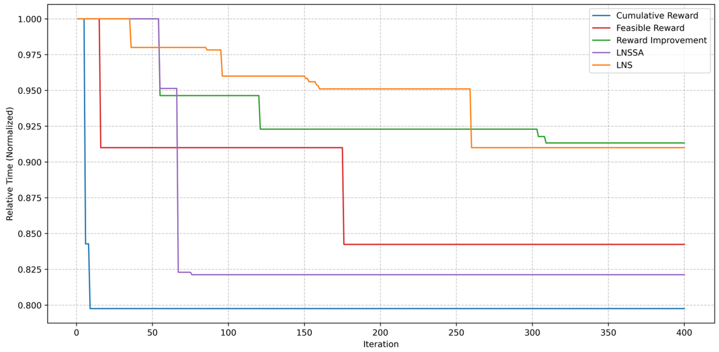
Due to structural differences among the compared algorithms, the Q-learning algorithm involves multiple time steps within each training episode (iteration), whereas heuristic algorithms such as LNS and LNSSA update the solution only once per iteration. To ensure comparability of the convergence processes across different algorithms in the plot, each Q-learning time step is treated as a single iteration unit, to ensure comparability when plotting the cumulative reward curve. Furthermore, to eliminate differences in initial objective values or reward magnitudes among the algorithms, all iterative curves are normalized by mapping the vertical axis of each curve to the [0,1] interval. This design ensures a unified scale on the horizontal axis and comparability on the vertical axis, allowing readers to intuitively assess the convergence speed and performance of each algorithm. In addition, the curves labeled ‘Reward Feasible’ and ‘Reward Improvement’ represent variants in which the cumulative reward mechanism is removed; that is, rewards are assigned only when a feasible solution is obtained or when an improvement over the current best solution occurs. Including these variants allows for a clear comparison of the effect of the cumulative reward mechanism on convergence behavior. Figure 8 presents the normalized iterative convergence curves of all algorithms. It is evident that the proposed method consistently converges to superior solutions across multiple runs, with faster convergence and smaller variance. This demonstrates that the cumulative reward mechanism effectively guides the learning process, enhancing both stability and solution quality.

4.3.2. Learning Rate Sensitivity

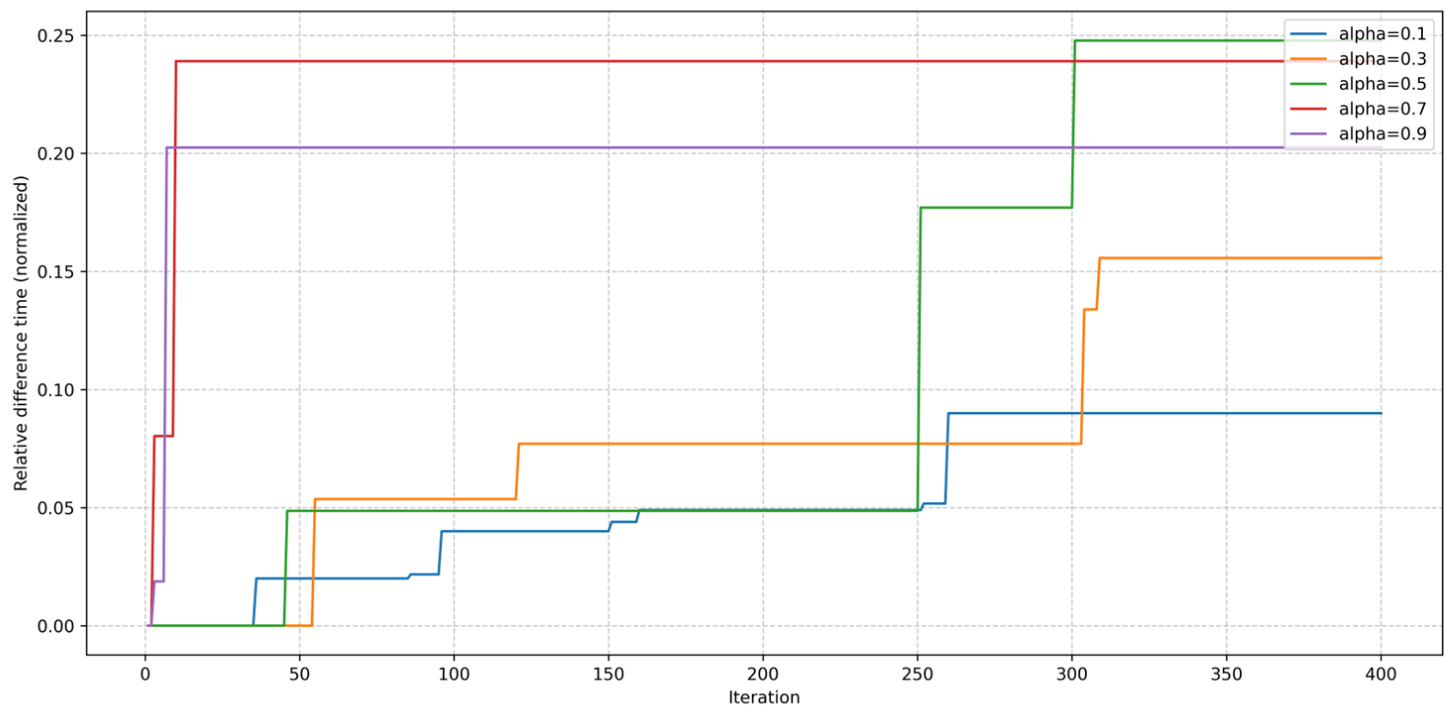
To analyze the impact of the learning rate α on the algorithm’s performance, we varied α within the set {0.1, 0.3, 0.5, 0.7, 0.9} while keeping other parameters unchanged. Each α value was tested in 10 independent experiments, and the final average objective value was recorded.
As shown in Figure 9, the learning rate significantly influences convergence behavior. A too-small α leads to slow learning and long convergence times; however, this does not mean that a larger α is always better. Experimental results indicate that α = 0.5 and α = 0.7 achieve a good balance between convergence speed and solution quality, providing practical guidance for parameter tuning in similar problems.

4.3.3. Theoretical Discussion

The classic Q-learning algorithm is proven to converge to the optimal policy under conditions including sufficient exploration of the state-action space and appropriate learning rate schedules. In our approach, the cumulative reward mechanism maintains the Markov property and preserves the theoretical convergence guarantees by:
Employing an ε-greedy exploration strategy to ensure all actions are explored adequately.
Selecting a fixed learning rate within a theoretically justified range to balance learning stability and adaptability.
While the cumulative reward design adds complexity, it aligns with the framework of discounted reward MDPs, and empirical results substantiate its effectiveness without sacrificing convergence properties.

4.4. Analysis of Driver Workload Balance

In addressing the balance of drivers’ workloads, we propose a simple empirical mechanism. Based on historical data and experience, we set a limit that a driver should not exceed for the number of tasks, known as A. We will now analyze this parameter further.
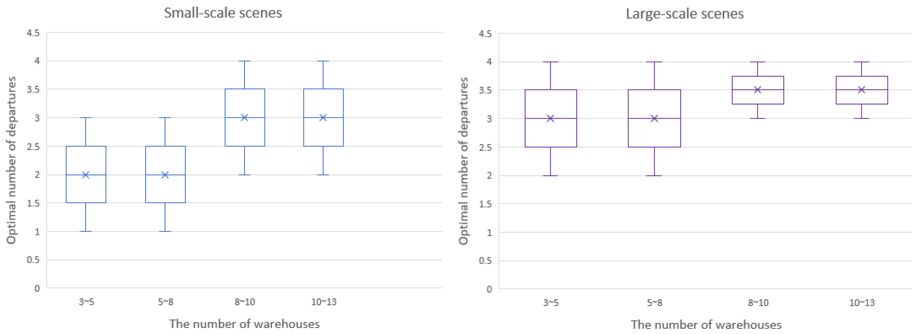
When workload balance is not taken into account, the presence of a heterogeneous fleet leads to two scenarios across different scales: Scenario 1: With ample time, all high-capacity vehicles are continuously in operation, which means the drivers have no rest. The advantage is that transportation tasks can be completed more quickly. Scenario 2: Due to an overwhelming demand, even with all high-capacity vehicle drivers working continuously, it is impossible to complete all transportation tasks within the time limit. We must mobilize other vehicles to ensure task completion. After testing, if we consider the constraint of driver workload balance, in small-scale cases, each driver can reduce their working hours by an average of 2.88%, and in the other scenario, by an average of 3.98%. Reduced working hours imply that drivers will be more passionate and creative at work, as shown in Figure 10. Reduced working hours imply that drivers will be more passionate and creative at work. In this paper, we use a simple empirical mechanism for driver workload balance, stipulating that each driver should not exceed three departures while prioritizing the use of larger vehicles to ensure transportation efficiency. We have questioned this empirical mechanism and sought to determine the optimal number of departures, A, in different scenarios. After calculation, it was found that setting A to 3 always yields acceptable overall performance. It is not difficult to see that A can be represented by the following formula. Let A represent the actual daily travel time, excluding any time-window constraints, and denote the average time required to complete a single trip. Figure 11 illustrates the values of A under two different scales.
A = T a c T a t

4.5. Fleet-Composition Analysis for a Heterogeneous Fleet

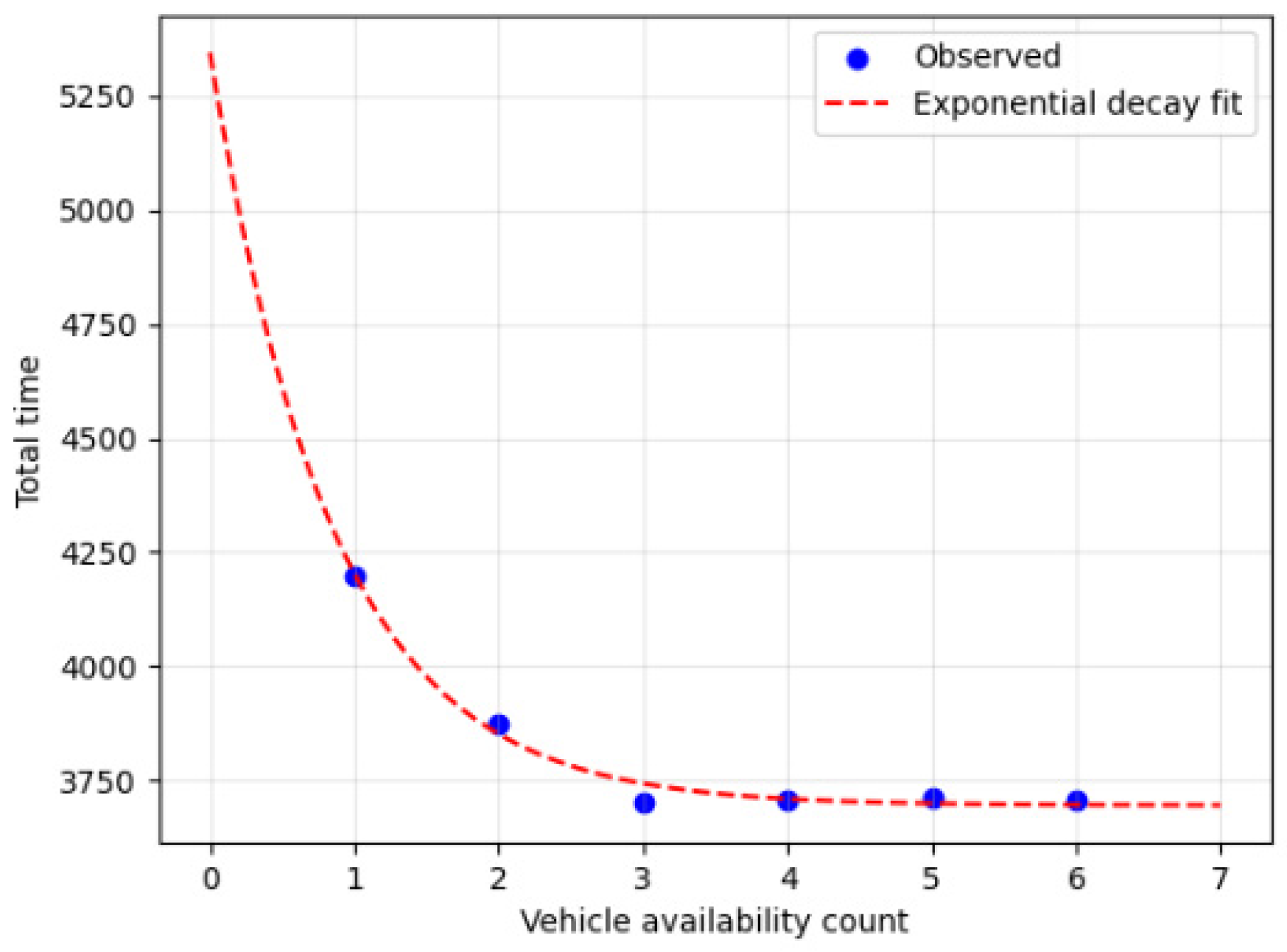
All large-capacity vehicles are currently company-owned, whereas all small-capacity vehicles are crowd-sourced. Fixing the total fleet size at its present maximum, we evaluate the current scale and composition. As shown in Figure 12, extreme strategies—either a fully crowd-sourced or a fully owned fleet—are found to incur markedly higher total time costs. This outcome stems from the negative impact that a bimodal time-varying (BTV) network exerts on any single vehicle type, thereby confirming the necessity of a heterogeneous fleet for efficient distribution.
Further observation reveals that, under small-scale operations, the total distribution completion time initially decreases and then increases as the proportion of crowd-sourced vehicles rises, reaching its minimum when this proportion is approximately two-thirds. In contrast, under large-scale conditions, the same proportion exhibits an opposite pattern: total distribution time first increases, then decreases, attaining its minimum at roughly three-fifths, followed by a renewed upward trend. Waiting time, while generally correlated with total distribution time, displays markedly higher volatility. Analysis indicates that, within a bimodal time-varying (BTV) network, crowd-sourced vehicles can indeed be deployed during both peak and off-peak periods; however, their limited capacity constrains aggregate throughput. Company-owned, large-capacity vehicles, although temporarily idle during peak hours, deliver superior transport efficiency once utilized.

4.6. Managerial Implications

Drawing upon the comprehensive sensitivity analyses and empirical results presented in Section 4.3 and Section 4.4, we distill the following evidence-based managerial implications for urban logistics operators confronting bimodal time-varying networks and heterogeneous multi-trip fleet environments.
1.
Institutionalize the Driver Trip Limit
Experimental evidence demonstrates that the imposition of a daily trip limit on drivers exerts a decisive influence on overall distribution efficiency. When total workload is held constant, either an excessively low or an excessively high ceiling on trip frequency impairs completion performance. Consequently, the allowable number of trips, A, should be codified as a non-negotiable, hard constraint within the dispatch system rather than treated as a flexible aspiration. From a workload perspective, this mechanism enforces a balanced allocation of effort while embodying a human-centered commitment to driver welfare.
2.
Dynamic Fleet Mix Governance
Extreme strategies—whether fully owned or fully crowd-sourced fleets—are consistently sub-optimal. Firms should implement a daily capacity-adjustment mechanism that dynamically optimizes the owned-to-outsourced ratio based on real-time demand forecasts and congestion indices. For small-scale operations, crowd-sourced fleets should account for approximately two-thirds of capacity, scaling to three-fifths in large-scale scenarios. This ensures minimal total logistics cost while maintaining service resilience.

5. Conclusions

We developed a mixed-integer programming (MIP) model that simultaneously considers traffic peaks, fleet heterogeneity, warehouse capacities, and workload balancing. The proposed HHCRQL algorithm integrates reinforcement learning with heuristic search within a Markov Decision Process (MDP) framework, thereby enhancing decision-making efficiency and effectively avoiding local optima. Extensive experiments demonstrate that HHCRQL consistently outperforms classical heuristic algorithms, metaheuristics, and commercial solvers in terms of solution quality, convergence speed, and robustness. In particular, the cumulative reward mechanism significantly improves learning efficiency and solution stability, offering a reliable approach to complex multi-objective routing optimization.
Despite its strong performance, HHCRQL is currently tailored for offline optimization and does not yet directly address dynamic or real-time routing variations. In addition, the experimental settings remain restricted to specific vehicle types and warehouse configurations. Future research could explore integrating HHCRQL with advanced reinforcement learning frameworks such as DQN, Actor–Critic methods, or Transformer-based RL to further improve its adaptability and efficiency. Extending the algorithm to B2C hybrid fleet scenarios and evaluating its robustness under uncertain, dynamic, or real-time environments would also be valuable directions. Moreover, embedding HHCRQL into human-in-the-loop scheduling systems could bridge automated optimization with practical decision-making, thereby strengthening both its applicability and real-world impact.

Author Contributions

Conceptualization, N.L. and X.W.; methodology, N.L., X.W. and X.J.; software, X.W.; validation, X.W.; formal analysis, N.L. and X.W.; investigation, N.L. and X.W.; resources, N.L.; data curation, N.L. and X.W.; writing—original draft preparation, X.W.; writing—review and editing, N.L. and X.W.; visualization, X.W.; supervision, N.L.; project administration, N.L.; funding acquisition, N.L. All authors have read and agreed to the published version of the manuscript.

Funding

This work was supported by the National Natural Science Foundation of China (72171032, 72172023) and Humanities and Social Sciences Fund of Chinese Ministry of Education (21YJA630048, 21YJAZH070).

Data Availability Statement

Data unavailable due to commercial confidentiality. Part of the data is in Appendix A.

Conflicts of Interest

The authors declare that they have no known competing financial interests or personal relationships that could have appeared to influence the work reported in this paper.

Appendix A

Table A1. Warehouse-related data.
WarehouseOperation Rate
Serial NumberLarge Cargo TruckSmall Cargo Van
Loading Rate (Cubic
Meters/
Minute)
Fixed Time
(Cubic
Meters/Minute)
Loading Rate
(Cubic Meters/
Minute)
Fixed Time
(Cubic Meters/
Minute)
s u p e r h u b ( 0 ) 1.5101.6710
11151.0615
21151.6715
31.78151.6715
41151.0615
51151.0615
61.78151.4815
71151.0615
81151.0615
91151.0615
101151.0615
111151.0615
1151.0615
n1151.0615
Table A2. Results of HHCRQL for real data instances.
RoundCarTaskTimeCarry
100-1-11330, 400, 777110
10-1-11330, 400, 777110
20-1-11330.400.770110
30-1-11330, 400, 777110
40-1-11360, 430, 70345
50-4-11360, 430, 69738.65
60-3-11360, 430, 68445
70-7-11360, 430, 70345
80-6-8-11360, 430, 673, 80721.02
90-9-11360, 430, 69639.26
200-1-11861, 931, 1257110
10-1-11861, 931, 1257110
20-1-11861, 931, 1257110
30-1-11861, 931, 1257110
40-1-11743, 813, 96045
50-5-11733, 810, 94633.37
60-2-4-10-11724, 810, 934, 1008, 109821.79
70-3-11743, 813, 93636.3
80-2-11844, 914, 103226.54
Algorithm A1 Large Neighborhood Search—Simulated Annealing
LNSSA Algorithm parameters: Initial temperature (T0), End time (Tend), Cooling rate (α), Acceptance rate (p)
Input: algorithm parameters
1. initial solution: Greedy strategy
2. update feasible: get feasible solutions
3. while ture:
4.     Destroy operation: choose different operation to destroy initial solution
5.     Repair operation: choose different operation to repair destroyed solution
6.     Swap operation: choose different operation to swap repaired solution
7.     if feasible
8.      break
9. end while
10. while T ≥ Tend
11. feasible solutions = update feasible (initial solution)
12. Record better solutions and Accept the worse solution with Acceptance rate (p)
13. satisfy criterion
14. END while
15. output: Optimal solution
Table A3. Part of the real data.
WarehouseDemand
1863.96
248.33
381.3
4170.91
533.37
625.35
745.45
823.98
9 39.26
100.95
110
120
130
Table A4. Parameter setting.
ParameterDemand
Epsilon0.1
alpha0.5
gamma0.9
Max_episodes20
Max_steps20
T1000
T_end10
q0.8
939.26
100.95
110
120
130

Appendix B

Appendix B.1. ILS Pseudocode

Function Iterated Local Search(max_iter):
  Initialize initial solution: task, car, carry, available
  best_task, best_car, best_carry, best_available = feasibility_check(task, car, carry, available)
  best_score = compute_total_time(best_task, best_car, best_carry)
  found_feasible = is_feasible(best_task)
 
  For iteration = 1 to max_iter:
    iteration_found_feasible = False
 
    For operator in [relocate, swap_nodes, two_opt]:
      new_task, new_car, new_carry = operator(best_task, best_car, best_carry, best_available)
      new_task, new_car, new_carry, feasible, new_available = feasibility_check(new_task, new_car, new_carry, best_available)
 
      If feasible:
        iteration_found_feasible = True
        score = compute_total_time(new_task, new_car, new_carry)
        If score < best_score:
          Update best_task, best_car, best_carry, best_available, best_score
 
    found_feasible = found_feasible OR iteration_found_feasible
 
  Return best_task, best_car, best_carry, best_available, best_score, found_feasible

Appendix B.2. Initial Defacilitation Code

function initial_solu(demand, capa175, capa96, available, capavehicle):
task, car, carry, available = single_node_visit(demand, capa175, capa96, available)
task, car, carry, available = save_method(task, car, carry, capavehicle, available)
return task, car, carry, available
# --------------------------
# Generate Feasible Solution
# --------------------------
function updata_feasible1(taskin, carin, carryin, availablein):
  if input solution is None:
    task, car, carry, available = initial_solu(demand, capa175, capa96, available, capavehicle)
  else:
    deep copy input to task, car, carry, available
 
  max_iterations (Set the number of iterations)
 
  for iteration = 1 to max_iterations:
    # Destruction operator
    if iteration is even:
      task, car, carry, destroy_list, available = destroy_by_load(task, car, carry, available)
else:
      task, car, carry, destroy_list, available = destroy_by_time(task, car, carry, available)
 
    # Repair operator
    if iteration is even:
      task, car, carry, destroy_list, available = repair_after_load_destroy(task, car, carry, destroy_list, available)
    else:
      task, car, carry, destroy_list, available = repair_by_merge_or_new(task, car, carry, destroy_list, available)
 
    # Correct carry structure
    carry = correct_carry_structure(task, carry)
 
    # Time and feasibility check
    time = node_time1(task, car, carry)
    task, car, carry, time_list, feasible, available = feasibility(task, car, carry, time, available)
 
    if feasible:
      vehicle_duration = total_time(task, car, time)
      return task, car, carry, time, available, True, vehicle_duration
 
  return task, car, carry, time, available, feasible, vehicle_duration
# --------------------------
# Example of Usage
# --------------------------
task, car, carry, available = initial_solu(demand, capa175, capa96, available, capavehicle)
taskout, carout, carryout, timeout, availableout, feasible = updata_feasible1(task, car, carry, available)

References

  1. Jamrus, T.; Wang, H.; Chien, C. Dynamic coordinated scheduling for supply chain under uncertain production time to empower smart production for Industry 3.5. Comput. Ind. Eng. 2020, 142, 106375. [Google Scholar] [CrossRef]
  2. Zhao, Z.; Lee, C.K.M.; Ren, J.; Tsang, Y. Quality of service measurement for electric vehicle fast charging stations: A new evaluation model under uncertainties. Transp. A Transp. Sci. 2025, 21, 2232044. [Google Scholar] [CrossRef]
  3. Nguyen, V.S.; Pham, Q.D.; Nguyen, T.H.; Bui, Q.T. Modeling and solving a multi-trip multi-distribution center vehicle routing problem with lower-bound capacity constraints. Comput. Ind. Eng. 2022, 172, 108597. [Google Scholar] [CrossRef]
  4. Friggstad, Z.; Mousavi, R.; Rahgoshay, M.; Salavatipour, M.R. Improved approximations for capacitated vehicle routing with unsplittable client demands. In Integer Programming and Combinatorial Optimization, Proceedings of the 23rd International Conference, IPCO 2022, Eindhoven, The Netherlands, 27–29 June 2022; Springer: Cham, Switzerland, 2020; Volume 13265, pp. 251–261. [Google Scholar]
  5. Qi, R.; Li, J.; Wang, J.; Jin, H.; Han, Y. QMOEA: A Q-learning-based multiobjective evolutionary algorithm for solving time-dependent green vehicle routing problems with time windows. Inf. Sci. 2022, 608, 178–201. [Google Scholar] [CrossRef]
  6. Li, M.; Zhao, P.; Zhu, Y.; Cai, K. A learning and searching integration approach for same-day delivery problem with heterogeneous fleets considering uncertainty. Transp. A Transp. Sci. 2024, 44, 1–44. [Google Scholar] [CrossRef]
  7. Kou, S.; Golden, B.; Bertazzi, L. Estimating optimal split delivery vehicle routing problem solution values. Comput. Oper. Res. 2024, 168, 106714. [Google Scholar] [CrossRef]
  8. François, V.; Arda, Y.; Crama, Y.; Laporte, G. Large neighborhood search for multi-trip vehicle routing. Eur. J. Oper. Res. 2016, 255, 422–441. [Google Scholar] [CrossRef]
  9. Agrawal, A.K.; Yadav, S.; Gupta, A.A.; Pandey, S. A genetic algorithm model for optimizing vehicle routing problems with perishable products under time-window and quality requirements. Decis. Anal. J. 2022, 5, 100139. [Google Scholar] [CrossRef]
  10. Zhang, H.; Zhang, Q.; Ma, L.; Zhang, Z.; Liu, Y. A hybrid ant colony optimization algorithm for a multi-objective vehicle routing problem with flexible time windows. Inf. Sci. 2019, 490, 166–190. [Google Scholar] [CrossRef]
  11. Ahmed, Z.H.; Yousefikhoshbakht, M. An improved tabu search algorithm for solving heterogeneous fixed fleet open vehicle routing problem with time windows. Alex. Eng. J. 2023, 64, 349–363. [Google Scholar] [CrossRef]
  12. Osorio-Mora, A.; Escobar, J.W.; Toth, P. An iterated local search algorithm for latency vehicle routing problems with multiple depots. Comput. Oper. Res. 2023, 158, 106293. [Google Scholar] [CrossRef]
  13. Kuo, R.J.; Luthfiansyah, M.F.; Masruroh, N.A.; Zulvia, F.E. Application of improved multi-objective particle swarm optimization algorithm to solve disruption for the two-stage vehicle routing problem with time windows. Expert Syst. Appl. 2023, 225, 120009. [Google Scholar] [CrossRef]
  14. Su, E.; Qin, H.; Li, J.; Pan, K. An exact algorithm for the pickup and delivery problem with crowdsourced bids and transshipment. Transp. Res. Part B Methodol. 2023, 177, 102831. [Google Scholar] [CrossRef]
  15. Zhou, H.; Qin, H.; Cheng, C.; Rousseau, L. An exact algorithm for the two-echelon vehicle routing problem with drones. Transp. Res. Part B Methodol. 2023, 168, 124–150. [Google Scholar] [CrossRef]
  16. Pan, B.; Zhang, Z.; Lim, A. Multi-trip time-dependent vehicle routing problem with time windows. Eur. J. Oper. Res. 2021, 291, 218–231. [Google Scholar] [CrossRef]
  17. Moon, I.; Salhi, S.; Feng, X. The location-routing problem with multi-compartment and multi-trip: Formulation and heuristic approaches. Transp. A Transp. Sci. 2020, 16, 501–528. [Google Scholar] [CrossRef]
  18. Yu, V.F.; Salsabila, N.Y.; Gunawan, A.; Handoko, A.N. An adaptive large neighborhood search for the multi-vehicle profitable tour problem with flexible compartments and mandatory customers. Appl. Soft Comput. 2024, 156, 111482. [Google Scholar] [CrossRef]
  19. You, J.; Wang, Y.; Xue, Z. An exact algorithm for the multi-trip container drayage problem with truck platooning. Transp. Res. Part E Logist. Transp. Rev. 2023, 175, 103138. [Google Scholar] [CrossRef]
  20. Sethanan, K.; Jamrus, T. Hybrid differential evolution algorithm and genetic operator for multi-trip vehicle routing problem with backhauls and heterogeneous fleet in the beverage logistics industry. Comput. Ind. Eng. 2020, 146, 106571. [Google Scholar] [CrossRef]
  21. Neira, D.A.; Aguayo, M.M.; De la Fuente, R.; Klapp, M.A. New compact integer programming formulations for the multi-trip vehicle routing problem with time windows. Comput. Ind. Eng. 2020, 144, 106399. [Google Scholar] [CrossRef]
  22. Liu, W.; Dridi, M.; Ren, J.; El Hassani, A.H.; Li, S. A double-adaptive general variable neighborhood search for an unmanned electric vehicle routing and scheduling problem in green manufacturing systems. Eng. Appl. Artif. Intell. 2023, 126, 107113. [Google Scholar] [CrossRef]
  23. Qin, W.; Zhuang, Z.; Huang, Z.; Huang, H. A novel reinforcement learning-based hyper-heuristic for heterogeneous vehicle routing problem. Comput. Ind. Eng. 2021, 156, 107252. [Google Scholar] [CrossRef]
  24. Xu, B.; Jie, D.; Li, J.; Yang, Y.; Wen, F.; Song, H. Integrated scheduling optimization of U-shaped automated container terminal under loading and unloading mode. Comput. Ind. Eng. 2021, 162, 107695. [Google Scholar] [CrossRef]
  25. Duan, J.; Liu, F.; Zhang, Q.; Qin, J. Tri-objective lot-streaming scheduling optimization for hybrid flow shops with uncertainties in machine breakdowns and job arrivals using an enhanced genetic programming hyper-heuristic. Comput. Oper. Res. 2024, 172, 106817. [Google Scholar] [CrossRef]
  26. Zhang, Z.; Wu, F.; Qian, B.; Hu, R.; Wang, L.; Jin, H. A Q-learning-based hyper-heuristic evolutionary algorithm for the distributed flexible job-shop scheduling problem with crane transportation. Expert Syst. Appl. 2023, 234, 121050. [Google Scholar] [CrossRef]
  27. Li, L.; Zhang, H.; Bai, S. A multi-surrogate genetic programming hyper-heuristic algorithm for the manufacturing project scheduling problem with setup times under dynamic and interference environments. Expert Syst. Appl. 2024, 250, 123854. [Google Scholar] [CrossRef]
  28. Li, J.; Ma, Y.; Gao, R.; Cao, Z.; Lim, A.; Song, W.; Zhang, J. Deep reinforcement learning for solving the heterogeneous capacitated vehicle routing problem. IEEE Trans. Cybern. 2022, 52, 13572–13585. [Google Scholar] [CrossRef]
  29. Zhang, Z.; Qi, G.; Guan, W. Coordinated multi-agent hierarchical deep reinforcement learning to solve multi-trip vehicle routing problems with soft time windows. IET Intell. Transp. Syst. 2023, 17, 2034–2051. [Google Scholar] [CrossRef]
  30. Shang, C.; Ma, L.; Liu, Y. Green location routing problem with flexible multi-compartment for source-separated waste: A Q-learning and multi-strategy-based hyper-heuristic algorithm. Eng. Appl. Artif. Intell. 2023, 121, 105954. [Google Scholar] [CrossRef]
  31. Xu, K.; Shen, L.; Liu, L. Enhancing column generation by reinforcement learning-based hyper-heuristic for vehicle routing and scheduling problems. Comput. Ind. Eng. 2025, 206, 111138. [Google Scholar] [CrossRef]
  32. Dastpak, M.; Errico, F.; Jabali, O. Off-line approximate dynamic programming for the vehicle routing problem with a highly variable customer basis and stochastic demands. Comput. Oper. Res. 2023, 159, 106338. [Google Scholar] [CrossRef]
  33. Wang, Y.; Hong, X.; Wang, Y.; Zhao, J.; Sun, G.; Qin, B. Token-based deep reinforcement learning for Heterogeneous VRP with Service Time Constraints. Knowl. Based Syst. 2024, 300, 112173. [Google Scholar] [CrossRef]
  34. Huang, N.; Li, J.; Zhu, W.; Qin, H. The multi-trip vehicle routing problem with time windows and unloading queue at depot. Transp. Res. Part E Logist. Transp. Rev. 2021, 152, 102370. [Google Scholar] [CrossRef]
  35. Fragkogios, A.; Qiu, Y.; Saharidis, G.K.D.; Pardalos, P.M. An accelerated benders decomposition algorithm for the solution of the multi-trip time-dependent vehicle routing problem with time windows. Eur. J. Oper. Res. 2024, 317, 500–514. [Google Scholar] [CrossRef]
  36. Blauth, J.; Held, S.; Müller, D.; Schlomberg, N.; Traub, V.; Tröbst, T.; Vygen, J. Vehicle routing with time-dependent travel times: Theory, practice, and benchmarks. Discret. Optim. 2024, 53, 100848. [Google Scholar] [CrossRef]
  37. Sun, B.; Chen, S.; Meng, Q. Optimizing first-and-last-mile ridesharing services with a heterogeneous vehicle fleet and time-dependent travel times. Transp. Res. Part E Logist. Transp. Rev. 2025, 193, 103847. [Google Scholar] [CrossRef]
  38. Gutierrez, A.; Labadie, N.; Prins, C. A Two-echelon Vehicle Routing Problem with time-dependent travel times in the city logistics context. EURO J. Transp. Logist. 2024, 13, 100133. [Google Scholar] [CrossRef]
  39. Lu, J.; Nie, Q.; Mahmoudi, M.; Ou, J.; Li, C.; Zhou, X.S. Rich arc routing problem in city logistics: Models and solution algorithms using a fluid queue-based time-dependent travel time representation. Transp. Res. Part B Methodol. 2022, 166, 143–182. [Google Scholar] [CrossRef]
  40. Coelho, V.N.; Grasas, A.; Ramalhinho, H.; Coelho, I.M.; Souza, M.J.F.; Cruz, R.C. An ILS-based algorithm to solve a large-scale real heterogeneous fleet VRP with multi-trips and docking constraints. Eur. J. Oper. Res. 2016, 250, 367–376. [Google Scholar] [CrossRef]
  41. Zhao, J.; Poon, M.; Tan, V.Y.F.; Zhang, Z. A hybrid genetic search and dynamic programming-based split algorithm for the multi-trip time-dependent vehicle routing problem. Eur. J. Oper. Res. 2024, 317, 921–935. [Google Scholar] [CrossRef]
  42. He, D.; Ceder, A.A.; Zhang, W.; Guan, W.; Qi, G. Optimization of a rural bus service integrated with e-commerce deliveries guided by a new sustainable policy in China. Transp. Res. Part E Logist. Transp. Rev. 2023, 172, 103069. [Google Scholar] [CrossRef]
  43. Vieira, B.S.; Ribeiro, G.M.; Bahiense, L. Metaheuristics with variable diversity control and neighborhood search for the Heterogeneous Site-Dependent Multi-depot Multi-trip Periodic Vehicle Routing Problem. Comput. Oper. Res. 2023, 153, 106189. [Google Scholar] [CrossRef]
  44. Li, K.; Liu, T.; Kumar, P.N.R.; Han, X. A reinforcement learning-based hyper-heuristic for AGV task assignment and route planning in parts-to-picker warehouses. Transp. Res. Part E Logist. Transp. Rev. 2024, 185, 103518. [Google Scholar] [CrossRef]
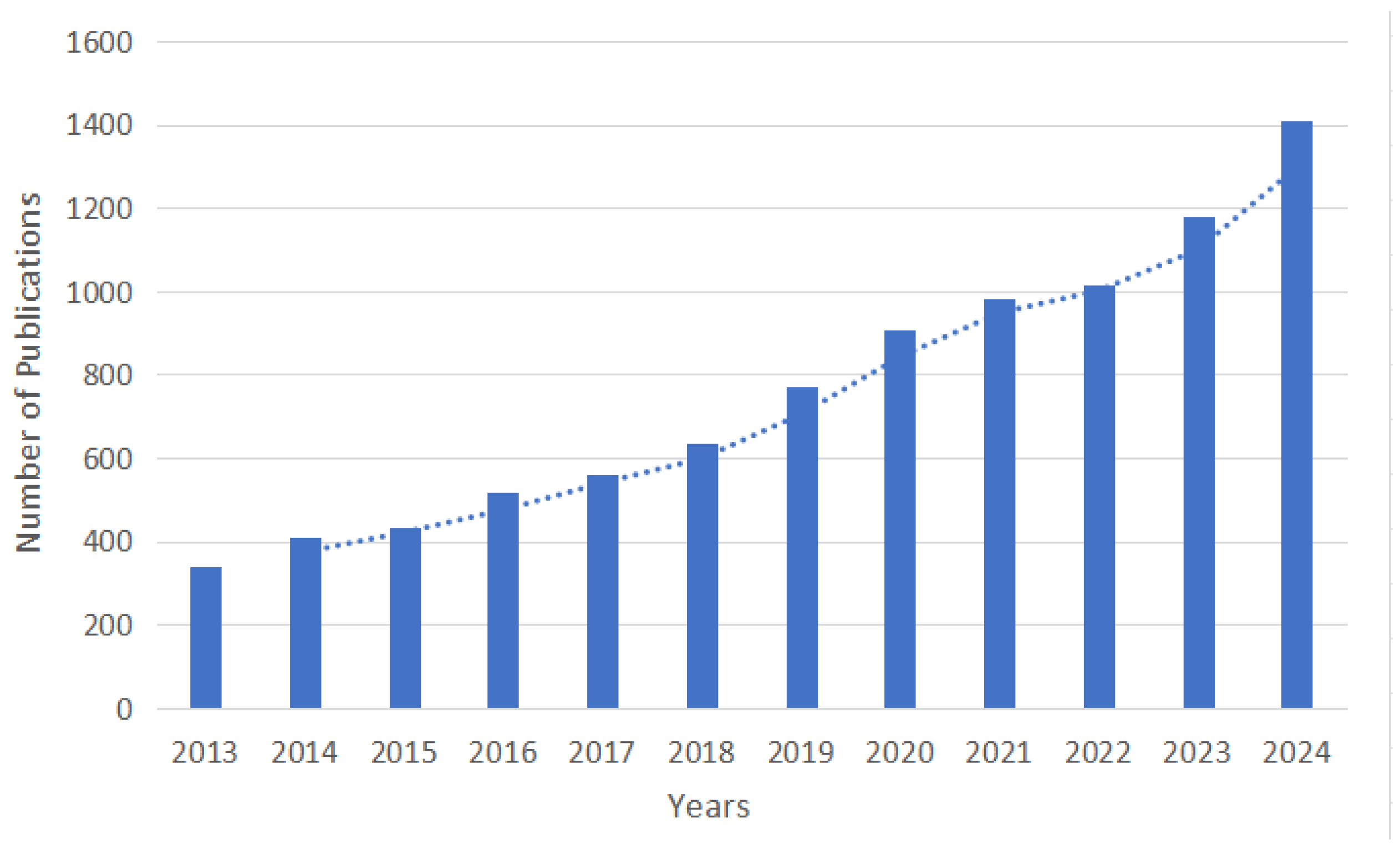
Figure 1. Annual number of MTVRP literature publications.
Algorithms 18 00536 g001
Figure 2. HO-RL framework.
Algorithms 18 00536 g002
Figure 3. Encoding of the solution.
Algorithms 18 00536 g003
Figure 4. One of the destroy operators.
Algorithms 18 00536 g004
Figure 5. One of the repair operators.
Algorithms 18 00536 g005
Figure 6. One of the swap operators.
Algorithms 18 00536 g006
Figure 7. An example of vehicle itineraries in the HMTVRPTW-TVN.
Algorithms 18 00536 g007
Figure 8. The iteration curves of multiple algorithms (relative).
Algorithms 18 00536 g008
Figure 9. The impact of learning rate α on convergence behavior (relative).
Algorithms 18 00536 g009
Figure 10. The impact of workload balance on target values.
Algorithms 18 00536 g010
Figure 11. Optimal driver workload across different scales.
Algorithms 18 00536 g011
Figure 12. Heterogeneous fleet-composition analysis.
Algorithms 18 00536 g012
Table 1. The related literature.
AuthorProblem CharacteristicsMethod
HFMulti-TripLCTVN
Nguyen et al. [3] AHA
Pan et al. [16] HMA
Yu et al. [18] ALNS
You et al. [19] BPC + PPC
Sethanan et al. [20] DE + FLC
Liu et al. [22] ALNS
Wang et al. [33] TDRL
Huang et al. [34] BPC + CG
Fragkogios et al. [35] BD
Blauth et al. [36] Local Search
Sun et al. [37] RHCG
Gutierrez et al. [38] HH
Lu et al. [39] BP
Coelho et al. [40] ILS
Zhao et al. [41] HH
He et al. [42] HH
Vieira et al. [43] AVNR
Our workHHCRQL
HF: heterogeneous fleet; TVN: time-varying network; LC: loading capacity; FLC: fuzzy logic controller; DE: differential evolution; BPC: branch-and-price-and-cut algorithm; PPC: pulse propagation algorithm; HMA: hybrid metaheuristic algorithm; ALNS: Adaptive Large Neighborhood Search; NLNS: Neural Large Neighborhood Search; AHA: Adaptive Heuristic Algorithm; HH: hybrid heuristics; HA: hybrid approaches; AVNR: Adaptive Variable Neighborhood Race; RHCG: rolling-horizon-based column generation; BP: branch-and-price: BD: benders decomposition; ILS: Iterated Local Search.
Table 2. The state set in MDP.
State VariableDescriptionPossible Values/IntervalsNotes
F Feasibility
Indicator
0/1Indicates whether the current solution
satisfies all constraints (1 = feasible, 0 =
infeasible)
V Number of
Vehicle Types
Discrete integers, e.g., 1, 2–3, ≥4Number of distinct vehicle types used,
reflecting fleet heterogeneity and problem complexity
T r Remaining Task Ratio[0, 0.25), [0.25, 0.5), [0.5, 0.75), [0.75, 1.0]Proportion of remaining demand relative to initial demand, representing progress stages
U Vehicle Load Utilization<33%, 33–66%, >66%Overall fleet load utilization intervals,
reflecting resource efficiency
Table 3. The action set in MDP.
ActionsHeuristic Operators
a 1 Destroy operation 1, repair operation 1, swap 1
a 2 Destroy operation 1, repair operation 1, swap 2
a 3 Destroy operation 1, repair operation 2, swap 1
a 4 Destroy operation 1, repair operation 2, swap 2
a 5 Destroy operation 2, repair operation 1, swap 1
a 6 Destroy operation 2, repair operation 1, swap 2
a 7 Destroy operation 2, repair operation 1, swap 1
a 8 Destroy operation 2, repair operation 2, swap 1
Table 4. Variables applied in the model.
VariablesDefinition
t i , j , k , q a c t u a l The actual travel time of small cargo van k from point i to point j
x i j k q The binary variable x i , j k , q equals 1 if vehicle k travels along arc ( i , j ) during its q_th trip; otherwise, it equals 0.
S i k q The arrival time of vehicle k at node i during its q_th trip.
d i k q The amount of goods picked up by vehicle k at node i during its q_th trip
w i k , q The waiting time of vehicle k at node i during its q_th trip
Z k q The binary variable equals 1 if vehicle k makes a q_th departure; otherwise, it equals 0.
T L k q The total load of Vehicle k on trip q
a i k , q Lunch break window auxiliary variable
b i k , q Lunch break window auxiliary variable.
y i , j , k , q 1 Small cargo van morning peak period indicator
(auxiliary variable)
y i , j , k , q 2 Small cargo van morning peak period indicator
(auxiliary variable)
z i , j , k , q Linearization auxiliary variables
Table 5. Parameters applied in the model.
ParametersDefinition
t i , j o r i g Normal travel time from node i to node j .
t i , j s m a l l Peak period travel time from node i to node j .
e i The loading and unloading capacity of warehouse i .
D T i k , q Departure time of vehicle k at node i during its q_th trip.
F T i The fixed working hours of warehouse i can be denoted as F T i .
c k The loading capacity of vehicle k can be denoted as c k
S T i The lower bound of the working time window for
warehouse i .
E T i The upper bound of the working time window for
warehouse i .
P T i The lower bound of the worker’s rest time window for warehouse i .
U T i The upper bound of the worker’s rest time window for warehouse i .
r T k The lower bound of the driver’s working time window for vehicle k .
R T k The upper bound of the driver’s working time window for vehicle k .
D D i The demand at warehouse i can be denoted as D D i
Q k The number of times vehicle k is used.
C The set of warehouses
D The distribution center
D s The origin distribution center
D e The destination distribution center
M The infinitely large constant
V The set of all nodes
KThe set of vehicles can be denoted as K
EThe set of arcs defined by ( i , j ) can be denoted as E
qThe number of vehicle departures can be denoted as q
AThe number of times a vehicle can be used
K s The set of small cargo van can be denoted as S.
K l The set of large cargo truck can be denoted as L
[ L T m , L T n ] The morning restricted time window for small cargo van
[ L T γ , L T δ ] The evening restricted time window for large cargo truck
[ T P m , T P n ] The morning peak time window for small cargo van
[ T P γ , T P δ ] The evening peak time window for large cargo truck
Table 6. Optimization analysis of actual scheduling results.
InstanceActual Solution (AS)Solution Derived from HHCRQL (HS) G A P
Number of
Warehouses
Total TimesWaiting TimesCar
Number
Total TimesWaiting TimesCar
Number
G a p 1 G a p 2
46944158710602411851213.25%25.33%
57481178412634512981315.19%27.24%
67854197815658714451716.13%26.95%
78120214517697615541914.09%27.55%
88478221519735917982013.20%18.83%
98752235419764018512112.71%21.37%
109352252420764019042218.31%24.56%
119531271020763718442219.87%31.96%
129778304120753420452322.95%32.75%
139965327824750621192424.68%35.36%
G a p 1 = ( T o t a l   t i m e A S T o t a l   t i m e H S ) / T o t a l   t i m e A S × 100 % . G a p 2 = ( W a i t i n g   t i m e A S W o t a l   t i m e H S ) / t o t a l   t i m e A S × 100 % .
Table 7. Small-scale calculation results.
InstanceThe Algorithm of the Solution
Number of
Warehouses
G u r o b i L N S L N S S A H H C R Q L G a p 3 G a p 4 G a p 5
Obj(s)CPU(s)Obj(s)CPU(s)Obj(s)CPU(s)Obj(s)CPU(s)--1
[0–5]910193.610090.589720.859320.39−2.36%8.26%4.29%
[5–10]18461635.520342.5219380.8518690.66−1.25%8.83%3.69%
[10–15]42912859.7454216.62450123.5442650.820.61%6.49%5.53%
[15–20]--507918.41487243.2046611.21-8.97%4.53%
[20–25]--711249.02689568.5265891.70-7.94%4.64%
[25–30]--761663.24746979.9770322.15-8.30%6.21%
[30–35]--11,839314.5211,252352.310,5502.97-12.22%6.65%
[35–40]--13,859561.313,489622.412,2273.85-13.35%10.32%
[40,45]--14,922744.214,525754.013,1494.03-13.48%10.46%
[45,50] 16,5241454.216,2451604.214,8954.35-10.94%9.06%
G a p 3 = ( O b j g u r o b i O b j H H C R Q L ) / O b j H H C R Q L × 100 % . G a p 4 = ( O b j L N S O b j H H C R Q L ) / O b j H H C R Q L × 100 % . G a p 5 = ( O b j L N S S A O b j H H C R Q L ) / O b j H H C R Q L × 100 % .
Table 8. Large-scale calculation results.
InstanceThe Algorithm of the Solution
Number of
Warehouses
I L S L N S LNS S A H H C R Q L G a p 6 G a p 7 G a p 8
Obj(s)CPU(s)Obj(s)CPU(s)Obj(s)CPU(s)Obj(s)CPU(s)--1
[50,55]17,366159517,058195216,854211815,9084.369.17%6.74%5.95%
[55,60]18,725207718,450210518,275235117,6524.786.08%4.33%3.53%
[60,65]19,625218519,300235019,216274518,7395.414.73%2.91%2.55%
[65,70]21,482221521,173245121,102278520,4755.874.92%3.30%2.57%
[70,75]22,041223721,763284121,630296521,0375.694.77%3.34%2.82%
[75,80]23,425226923,156289422,931310222,5205.474.02%2.75%1.83%
[80,85]24,495215424,207273423,997294123,6954.913.38%2.12%1.27%
[85,90]25,954219825,633296525,413321025,1245.953.30%1.99%1.15%
[90,95]27,658218427,258293627,137335426,7105.563.55%2.01%1.60%
[95,100]28,965223628,496281228,386324727,8745.723.91%2.18%1.84%
G a p 6 = O b j ILS O b j H H C R Q L / O b j H H C R Q L × 100 % . G a p 7 = O b j LNS O b j H H C R Q L / O b j H H C R Q L × 100 % . G a p 8 = ( O b j L N S S A O b j H H C R Q L ) / O b j H H C R Q L × 100 % .
Disclaimer/Publisher’s Note: The statements, opinions and data contained in all publications are solely those of the individual author(s) and contributor(s) and not of MDPI and/or the editor(s). MDPI and/or the editor(s) disclaim responsibility for any injury to people or property resulting from any ideas, methods, instructions or products referred to in the content.